Adaptive fuzzy control of time-varying impedance in rehabilitation exercises

Abstract

Time-varying impedance control is pivotal in shaping the dynamics of both patients and robots concurrently, facilitating tailored training for rehabilitation within human–robot interaction (HRI) scenarios, particularly for exoskeleton robots. Given the diverse physical characteristics of patients, sudden movement variations can pose challenges, potentially disrupting the robot’s functionality. Moreover, the inherent dynamics of robots coupled with uncertainties present additional hurdles for ensuring optimal and safe rehabilitation exercises. In this study, we introduce a novel approach: fuzzy adaptive time-varying impedance control, adept at mitigating external disturbances and addressing all uncertainties associated with both robot and patient dynamics, thereby ensuring safe and effective rehabilitation protocols. A primary concern with time-varying impedance control lies in system stability. Leveraging Lyapunov stability analysis, we delineate the safe operational boundaries of time-varying impedance control, thus averting potential instability. Our proposed impedance modulation facilitates desired dynamics while facilitating passive and isometric exercises for patients. Through simulations conducted in MATLAB2023, we demonstrate the efficacy of our approach, comparing its performance against conventional constant impedance control methods and also we used the controller for three different patients with various physical features that shows good results for all of them.

Keywords

Time-varying impedance rehabilitation robot HRI uncertainties disturbance fuzzy adaptive control

Introduction

Impedance control has emerged as a highly effective method for managing the interaction dynamics between robots and humans. It revolves around establishing a dynamic relationship between the force of interaction and various parameters such as acceleration, velocity, and displacement of both the robot and the associated body. In the realm of rehabilitation robotics, impedance control stands out as a viable strategy. By manipulating its dynamic model alongside the patient’s body, the robot can administer tailored exercises conducive to optimal rehabilitation outcomes.

While many existing approaches in rehabilitation literature lean toward constant impedance control (Akdogan and Arif, 2011), variable impedance control offers greater flexibility in modulating impedance profiles to align with desired dynamic models and enhance the robot’s resilience during environmental interactions (Ajoudani et al., 2012; Ficuciello et al., 2015). However, the paramount concern with variable impedance control lies in ensuring system stability (Sun et al., 2019). Exceeding appropriate bounds with variable terms can precipitate instability, a critical issue in the context of rehabilitation robotics with potentially catastrophic consequences.

The coefficients within the impedance equation represent the key parameters that can be varied during interaction. These coefficients—namely inertia, damping, and spring constants—correspond to acceleration, velocity, and displacement signals, respectively. Admittance control, as explored by Ficuciello et al. (2015) and Muller et al. (2018), offers an alternative perspective on impedance control, emphasizing the control of end effector velocity. In these studies, the spring coefficient is disregarded, while the inertia term remains constant, and only the damping coefficient varies inversely with end effector velocity.

In the studies by Lee and Buss (2008) and Kim et al. (2016), variable impedance control to achieve desired force output has been adopted. Here, the spring coefficient dynamically adjusts as the end effector seeks to exert a specified force, while the inertia and damping coefficients remain fixed. In the studies by Oguztöreli and Stein (1991) and Farahat and Herr (2010), a nonlinear spring coefficient that increases proportionally to the muscle force tolerated has been introduced. In the study by Tsumugiwa et al. (2002), a virtual mass and damper system to measure the patient’s spring coefficient, enabling dynamic adjustment of damping coefficient to regulate varying impedance has been employed. In the study by Li et al. (2016), electromyography (EMG) signals to estimate joint stiffness, employing an adaptive controller to facilitate rehabilitation have been utilized.

In the study by Furui et al. (2021), a lambda-type muscle model to redefine spring and damping coefficients during muscle relaxation has been implemented. In the study by Mersha et al. (2014), aerial interaction with variable impedance control, where spring coefficient variations drive changes in damping, while inertia remains constant has been explored. Ajoudani et al. (2012) selected spring coefficients proportional to EMG signals. Ikeura et al. (2002) optimized damping term using algorithms. In the studies by Yang et al. (2011), Burdet et al. (2014), Liang et al. (2014) and Li et al. (2018), learning approaches and adaptive controllers to mimic human behavior have been adopted.

Ensuring suitable coefficient ranges is crucial for maintaining system stability in variable impedance control. Ferraguti et al. (2013) and Zheng et al. (2018) introduced an energy tank-based method, utilizing a time-varying spring to stabilize the system. Kronander and Billard (2016) addressed coefficient ranges, treating inertia as constant, albeit with assumptions regarding interaction force. Sun et al. (2019) employed approximate dynamic inversion to model uncertainties, ensuring semi-global practical exponential stability. Liang et al. (2022) defined time-varying stiffness and employed an adaptive controller to manage uncertainty. Hamedani et al. (2021) adjusted stiffness based on force levels, utilizing a neural-fuzzy controller to estimate contact force. Jin and Guo (2023) used an extended state observer (ESO) and model predictive controller (MPC) for estimation of the uncertainty and disturbances of the patients during the lower limb rehabilitation by an exoskeleton robot. This robot has two links and after linearization could use the MPC for predicting the movements of the patients during rehabilitation.

Dong and Ren (2017) introduced a dynamic impedance curve with all coefficients varying over time, employing an uncertainty and disturbance estimator (UDE) to manage uncertainties. In this estimator, just the inertia matrix of the robot is considered to be uncertain and the UDE is defined by this assumption. Many studies focused on adapting impedance coefficients to ensure system stability. Huang and Chen (1992) used varying impedance with two strategies of position-based and force-based and could design the impedance coefficients to have a stable system. Park and Lee (2004) used adaptive control for control of a haptic device and could estimate the force in contact with people. Chien and Huang (2004) could use the adaptive impedance control to estimate the parameters of robot while the system became stable. Sharifi et al. (2014) utilized a model reference that finally led the adaptive control to have a stable system. Li et al. (2017) and Fateh and Khoshdel (2015) used the adaptive impedance control to change the impedance coefficients to have a stable system. However, these time-varying coefficients are not desired to be the best dynamic behavior of the system that can be satisfying for the specified usage. This research is trying to change the impedance parameter to get the force or the position of the robot to the desired amount in the presence of uncertainty and keep the system stable.

This study aims to adapt impedance parameters to achieve desired force or position in the presence of uncertainty while maintaining system stability. A new adaptive fuzzy controller is proposed to guide rehabilitation robots amid uncertainty and patient limb disturbances. Through time-varying impedance control, the robot can mimic professional physiotherapists’ behavior during training, providing variable impedance ratios for effective interaction. Simulation results demonstrate the controller’s efficacy in tracking desired impedance while ensuring system stability.

The paper proceeds as follows: The section “Problem formulation” presents robot dynamics and its conversion to a Cartesian coordinate system. The section “Time-varying impedance control” details the time-varying impedance control concept and the utilization of adaptive fuzzy control to achieve desired impedance. The section “Simulation” showcases simulation results and evaluates the proposed method’s effectiveness. Finally, the section “Conclusion and future research” offers concluding remarks.

Problem formulation

We consider an electrically driven rehabilitation robot comprising n links interconnected at n joints within an open kinematic chain. Each link is actuated by a permanent magnet direct current (DC) motor via gears. We make the idealized assumption that both the links and the couplings between the electric motors and links exhibit perfect rigidity. The dynamic model governing the system is expressed as shown in equation (1)

D_{r} (q) \overset{\cdot\cdot}{q} + C_{r} (q, \overset{\cdot}{q}) \overset{\cdot}{q} + G_{r} (q) + τ_{e} + φ_{τ} = τ_{r}

(1)

where $q ϵ R^{n}$ is the vector of joint positions, $D_{r} (q) ϵ R^{n}$ is the matrix of robot inertia, $C_{r} (q, \overset{\cdot}{q}) ϵ R^{n}$ is the vector of centrifugal and Coriolis torques, $G_{r} (q) ϵ R^{n}$ is the vector of gravitational torques, $τ_{e} ϵ R^{n}$ is the vector of the load torque, and $τ_{r} ϵ R^{n}$ is the torque vector of the robot. $φ_{τ}$ is external disturbances that can be the movements of the patient during the rehabilitation exercise. The load torque is actually provided by the human lower limb located on the robot and we have

D_{e} (q) \overset{\cdot\cdot}{q} + C_{e} (q, \overset{\cdot}{q}) \overset{\cdot}{q} + G_{e} (q) - J^{T} (q) F_{h} = τ_{e}

(2)

where, $D_{e} (q) ϵ R^{n}$ is the inertia matrix of the human’s body, $C_{e} (q, \overset{\cdot}{q}) ϵ R^{n}$ is the vector of centrifugal and Coriolis torques of the human body, $G_{e} (q) ϵ R^{n}$ is the vector of gravitational torques of the human body, $F_{h} ϵ R^{n}$ is the vector of the generated forces by humans. As the rehabilitation robots are in the category of exoskeleton robots and in the rehabilitation process, the human and robot become one rigid body; the mechanical subsystem of the rehabilitation robot is obtained by substituting equation (2) into equation (1) in the form of

D (q) \overset{\cdot\cdot}{q} + C (q, \overset{\cdot}{q}) \overset{\cdot}{q} + G (q) - J^{T} (q) F_{h} + φ_{τ} = τ_{r}

(3)

in which

D (q) = D_{e} (q) + D_{r} (q)

(4)

C (q, \overset{\cdot}{q}) = C_{e} (q, \overset{\cdot}{q}) + C_{r} (q, \overset{\cdot}{q})

(5)

G (q) = G_{e} (q) + G_{r} (q)

(6)

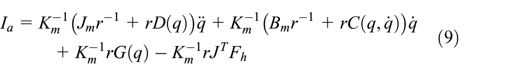
The electric motors provide the joint torques of the robot as follows

J_{m} r^{- 1} \overset{\cdot\cdot}{q} + B_{m} r^{- 1} \overset{\cdot}{q} + r τ_{r} = K_{m} I_{a}

(7)

I_{a} = K_{m}^{- 1} (J_{m} r^{- 1} \overset{\cdot\cdot}{q} + B_{m} r^{- 1} \overset{\cdot}{q} + r τ_{r})

(8)

From equations (3) and (8), it is concluded that

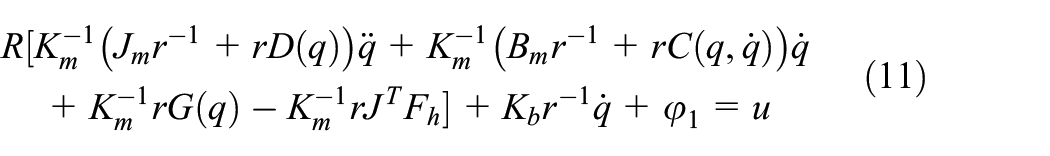
\begin{matrix} I_{a} = K_{m}^{- 1} (J_{m} r^{- 1} + rD (q)) \overset{\cdot\cdot}{q} + K_{m}^{- 1} (B_{m} r^{- 1} + rC (q, \overset{\cdot}{q})) \overset{\cdot}{q} \\ + K_{m}^{- 1} rG (q) - K_{m}^{- 1} r J^{T} F_{h} \end{matrix}

(9)

In a permanent magnet DC motor, the electrical equation is given by

R I_{a} + L {\overset{\cdot}{I}}_{a} + K_{b} r^{- 1} \overset{\cdot}{q} + φ = u

(10)

where $φ ϵ R^{n}$ is the external disturbance that shows the external disturbance in equation (1) is changed to the electrical load. From equations (9) and (10), we have

\begin{matrix} R [K_{m}^{- 1} (J_{m} r^{- 1} + rD (q)) \overset{\cdot\cdot}{q} + K_{m}^{- 1} (B_{m} r^{- 1} + rC (q, \overset{\cdot}{q})) \overset{\cdot}{q} \\ + K_{m}^{- 1} rG (q) - K_{m}^{- 1} r J^{T} F_{h}] + K_{b} r^{- 1} \overset{\cdot}{q} + φ_{1} = u \end{matrix}

(11)

in which $, φ_{1} = L {\overset{\cdot}{I}}_{a} + φ$ . Using the Jacobian matrix of a robot manipulator, the relations between the task space and joint space are given by

\overset{\cdot}{X} = J \overset{\cdot}{q}

(12)

\overset{\cdot}{q} = J^{- 1} \overset{\cdot}{X}

(13)

\overset{\cdot\cdot}{X} = \overset{\cdot}{J} \overset{\cdot}{q} + J \overset{\cdot\cdot}{q}

(14)

\overset{\cdot\cdot}{q} = J^{- 1} (\overset{\cdot\cdot}{X} - \overset{\cdot}{J} \overset{\cdot}{q})

(15)

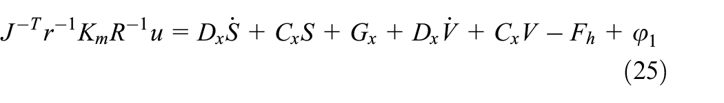
Based on these equations, the robot motion equation in the task space is given by

J^{- T} r^{- 1} K_{m} R^{- 1} u = D_{x} \overset{\cdot\cdot}{x} + C_{x} \overset{\cdot}{x} + G_{x} - F_{h} + φ_{1}

(16)

where

\begin{matrix} D_{x} = J^{- T} r^{- 1} (J_{m} r^{- 1} + rD (q)) J^{- 1} \\ \begin{matrix} C_{x} = J^{- T} r^{- 1} (B_{m} r^{- 1} + rC (q, \overset{\cdot}{q})) J^{- 1} + J^{- T} r^{- 1} K_{m} R^{- 1} K_{b} r^{- 1} J^{- 1} \\ - J^{- T} r^{- 1} (J_{m} r^{- 1} + rD (q)) \overset{\cdot}{J} J^{- 1} \end{matrix} \\ G_{x} = J^{- T} {RK}_{m}^{- 1} rG (q) \end{matrix}

(17)

The time-varying impedance control

The controller presented in this paper comprises two distinct components. The first component, serving as the inner controller, embodies the impedance model tasked with managing the dynamic interplay between the robot and the patient. Meanwhile, the outer layer of the controller entails the adaptive controller, designed to mitigate the impact of uncertainties and disturbances. The overarching objective of the outer layer controller is to drive the system’s state variables toward the desired impedance amid the presence of uncertainties and disturbances. To achieve this objective, an error term is defined, acting as a pivotal metric for assessing the deviation between the desired and actual system states

E_{out} = X - X_{i}

(18)

Now a sliding surface is designed as follows

S = {\overset{\cdot}{E}}_{out} + A E_{out} = \overset{\cdot}{X} - {\overset{\cdot}{X}}_{i} + A E_{out}

(19)

and the control effort is such that $S$ reaches zero. Thus, we have

\overset{\cdot}{S} = {\overset{\cdot\cdot}{E}}_{out} + A {\overset{\cdot}{E}}_{out} = \overset{\cdot\cdot}{X} - {\overset{\cdot\cdot}{X}}_{i} + A {\overset{\cdot}{E}}_{out}

(20)

Similarly, we use an auxiliary variable called $V$ , which is defined as follows

V = {\overset{\cdot}{X}}_{i} - A E_{out}

(21)

\overset{\cdot}{V} = \overset{\cdot\cdot}{X} i - A {\overset{\cdot}{E}}_{out}

(22)

From equations (18)–(21), it follows that

{\overset{\cdot}{X}}_{i} = S + V

(23)

{\overset{\cdot\cdot}{X}}_{i} = \overset{\cdot}{S} + \overset{\cdot}{V}

(24)

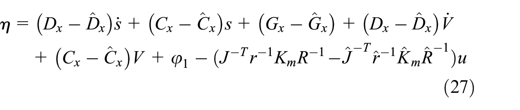
By replacing equations (23) and (24) in equation (16), we have

J^{- T} r^{- 1} K_{m} R^{- 1} u = D_{x} \overset{\cdot}{S} + C_{x} S + G_{x} + D_{x} \overset{\cdot}{V} + C_{x} V - F_{h} + φ_{1}

(25)

By considering uncertainty and nominal models, the motion equation is given by

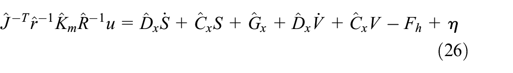
{\hat{J}}^{- T} {\hat{r}}^{- 1} {\hat{K}}_{m} {\hat{R}}^{- 1} u = {\hat{D}}_{x} \overset{\cdot}{S} + {\hat{C}}_{x} S + {\hat{G}}_{x} + {\hat{D}}_{x} \overset{\cdot}{V} + {\hat{C}}_{x} V - F_{h} + η

(26)

The above equation is the nominal model of the system and $η$ is the term in which the difference between the real and estimated system is included

\begin{matrix} η = (D_{x} - {\hat{D}}_{x}) \overset{\cdot}{s} + (C_{x} - {\hat{C}}_{x}) s + (G_{x} - {\hat{G}}_{x}) + (D_{x} - {\hat{D}}_{x}) \overset{\cdot}{V} \\ + (C_{x} - {\hat{C}}_{x}) V + φ_{1} - (J^{- T} r^{- 1} K_{m} R^{- 1} - {\hat{J}}^{- T} {\hat{r}}^{- 1} {\hat{K}}_{m} {\hat{R}}^{- 1}) u \end{matrix}

(27)

The inner layer of the controller tries to bring the dynamic equation of system impedance to the desired dynamic equation. The designed impedance model is as follows

M_{i} (t) ({\overset{\cdot\cdot}{x}}_{d} - {\overset{\cdot\cdot}{x}}_{i}) + B_{i} (t) ({\overset{\cdot}{x}}_{d} - {\overset{\cdot}{x}}_{i}) + K_{i} (t) (x_{d} - x_{i}) = F_{h}

(28)

E_{in} = x_{d} - x_{i}

(29)

where, $K_{i} (t)$ , $M_{i} (t)$ , and $B_{i} (t)$ are diagonal matrices that can be considered as impedance parameters. These time-varying parameters can have every desired profile and change the dynamic model of robot and the patient to the desired model. The following control law is suggested to control the system

\begin{matrix} u = \hat{R} {\hat{K}}_{m}^{- 1} \hat{r} {\hat{J}}^{T} ({\hat{G}}_{x} + {\hat{D}}_{x} \overset{\cdot}{V} + {\hat{C}}_{x} V - KS + u_{fuzzy} \\ - (M_{i} (t) ({\overset{\cdot\cdot}{x}}_{d} - {\overset{\cdot\cdot}{x}}_{i}) + B_{i} (t) ({\overset{\cdot}{x}}_{d} - {\overset{\cdot}{x}}_{i}) + K_{i} (t) (x_{d} - x_{i}))) \end{matrix}

(30)

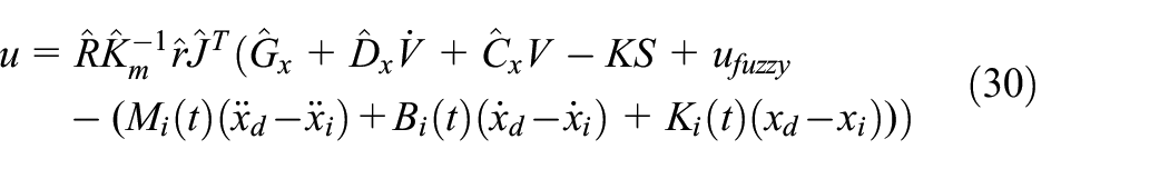
When this control law imposes on the system given by equation (25), the result will be as follows

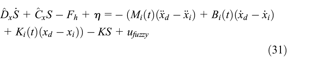
\begin{matrix} {\hat{D}}_{x} \overset{\cdot}{S} + {\hat{C}}_{x} S - F_{h} + η = - (M_{i} (t) ({\overset{\cdot\cdot}{x}}_{d} - {\overset{\cdot\cdot}{x}}_{i}) + B_{i} (t) ({\overset{\cdot}{x}}_{d} - {\overset{\cdot}{x}}_{i}) \\ + K_{i} (t) (x_{d} - x_{i})) - KS + u_{fuzzy} \end{matrix}

(31)

The equation (31) is divided into two parts as given below

(i) {\hat{D}}_{x} \overset{\cdot}{S} + {\hat{C}}_{x} S + KS = u_{fuzzy} - η = ξ \hat{P} - ξ P = ξ \tilde{P}

(32)

(ii) Equation (28), that is, impedance dynamic equation, where

u_{fuzzy} = ξ \hat{P}

(33)

ξ = [\begin{matrix} ξ_{1}^{T} & 0 \\ 0 & ξ_{2}^{T} \end{matrix}] \hat{P} = [\begin{matrix} {\hat{P}}_{1} \\ {\hat{P}}_{2} \end{matrix}]

(34)

And $u_{fuzzy}$ compensates the terms related to complex uncertainty and $K$ is a 2×2 diagonal matrix. By applying the control law to the system and forming a closed loop, we have

{\hat{D}}_{x} \overset{\cdot}{S} = ξ \tilde{P} - {\hat{C}}_{x} S - KS

(35)

Here, the fuzzy system is used to eliminate the effect of disturbance and uncertainty. This fuzzy system tries to minimize the effect of uncertainties. The most important principle in the design of the fuzzy system is the selection of system inputs, in this system the two inputs are $S$ and $\overset{\cdot}{S}$ and their values are known according to equations (19) and (20). For each of the inputs of the fuzzy system, three membership groups are considered.

Assuming $\hat{F}$ represents the output of an adaptive fuzzy system in normalized form, with inputs $S$ and $\overset{\cdot}{S}$ , covering the entire control space with nine fuzzy rules can be achieved by employing three fuzzy sets for each input. These linguistic fuzzy rules, proposed in Mamdani style, follow the format

F R_{1} : If S is A_{l} and \overset{\cdot}{S} is B_{l} Then \hat{F} is C_{l}

(36)

For $S$ , three Gaussian membership functions—Positive (P), Zero (Z), and Negative (N)—are defined within the manipulator’s operational range. Similarly, three Gaussian membership functions—P, Z, and N—are used for input $\overset{\cdot}{S}$ . Nine symmetric Gaussian membership functions, namely very positive high (VPH), positive high (PH), positive medium (PM), positive small (PS), zero (Z), negative small (NS), negative medium (NM), negative high (NH), and very negative high (VNH), are defined for $\hat{F}$ using the form

μ_{l} (\hat{F}) = \exp (- {(\frac{\hat{F} - {\hat{p}}_{l}}{σ})}^{2})

(37)

for $l = 1, . . ., 9$ within the output’s operational range. Here, the symmetric Gaussian function relies on parameters ${\hat{p}}_{l}$ and $σ$ , with ${\hat{p}}_{l}$ being adapted by an adaptive law, while $σ$ remains a constant. As a result, the entire space of the fuzzy system is covered with nine control rules, whose form is shown below. Figure 1(a) shows input $S$ and Figure 1(b) shows $\overset{\cdot}{S}$ :

Figure 1.

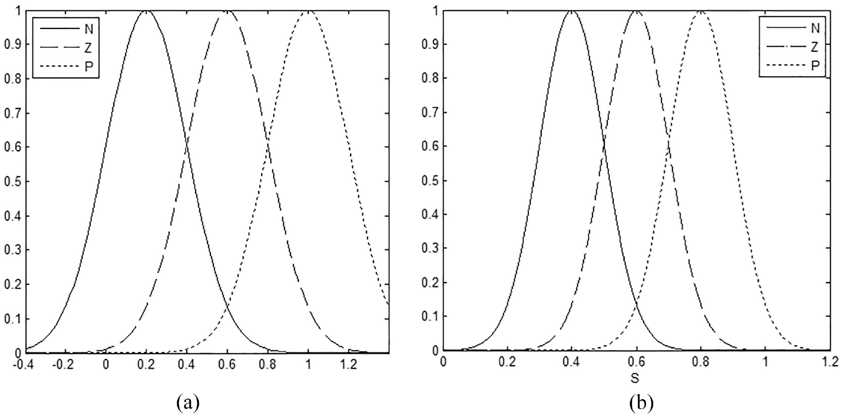
Fuzzy inputs (a) $S$ and (b) $\overset{\cdot}{S}$ .

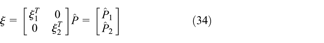
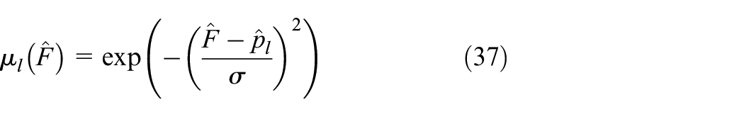
If we use the Mamdani-type inference engine, the Gaussian fuzzifier and the center average defuzzifier, the output will be

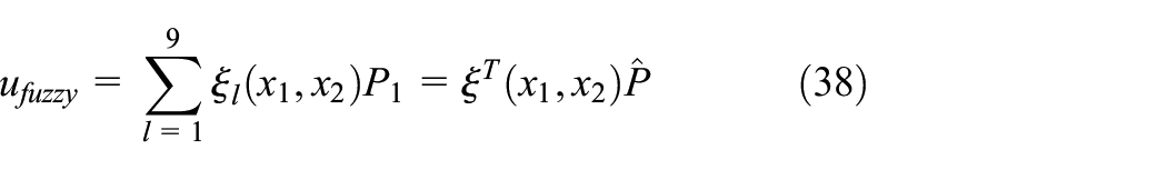
u_{fuzzy} = \sum_{l = 1}^{9} ξ_{l} (x_{1}, x_{2}) P_{1} = ξ^{T} (x_{1}, x_{2}) \hat{P}

(38)

where, $ξ$ and $\hat{P}$ are defined in equation (34). When $Ψ = [Ψ_{1} \dots Ψ_{9}]$ , which is a positive value and is calculated as follows

ξ_{1} (x_{1}, x_{2}) = \frac{μ_{A_{l}} (x_{1}) μ_{B_{l}} (x_{2})}{\sum_{l = 1}^{9} μ_{A_{l}} (x_{1}) μ_{B_{l}} (x_{2})}

(39)

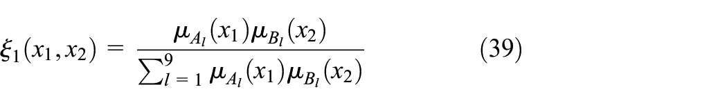
where, $μ_{A_{l}}$ , $μ_{B_{l}}$ , $x_{1}$ , $x_{2}$ [0,1] are the first term of $S$ and $\overset{\cdot}{S}$ .

Stability stands as the primary concern in time-varying impedance controllers. The incremental adjustment of impedance over time carries the risk of inducing instability, a particularly untenable scenario in medical robotics. While certain impedance coefficients have been identified as stabilizers for adaptive systems (Chien and Huang, 2004; Huang and Chen (1992); Li et al., 2017; Park and Lee, 2004; Sharifi et al., 2014), they often merely ensure stability without necessarily achieving the desired interaction dynamics. These coefficients are adjusted to a specific extent to maintain system stability, yet they may not fully address the dynamic requirements for interaction. In the study by Dong and Ren (2017), Dong tackled this issue by proposing specific limits for inertia, damping, and spring coefficients. These limits not only ensure the stability of the time-varying system but also allow all coefficients to be dynamically adjusted, facilitating attainment of desired dynamics within specified limits. Dong’s approach serves as a source of inspiration for this paper.

Dong considered the inertia matrix as a parameter fraught with uncertainty, a characteristic shared by all robot components in this article. To address this uncertainty, an adaptive control mechanism employing a fuzzy adaptive controller is introduced. In order to establish stability and derive adaptive rules, compensation based on Lyapunov’s function is proposed

L = L_{1} + L_{2}

(40)

L_{1} = \frac{1}{2} {E_{in}}^{T} β (t) E_{in} + \frac{1}{2} {({\overset{\cdot}{E}}_{in} + α E_{in})}^{T} M_{i} (t) ({\overset{\cdot}{E}}_{in} + α E_{in})

(41)

L_{2} = \frac{1}{2} S^{T} {\hat{D}}_{x} S + \frac{1}{2 λ} {\tilde{P}}^{T} P

(42)

\begin{matrix} L = \frac{1}{2} S^{T} {\hat{D}}_{x} S + \frac{1}{2 λ} {\tilde{P}}^{T} \tilde{P} + \frac{1}{2} {E_{in}}^{T} β (t) E_{in} + \frac{1}{2} {({\overset{\cdot}{E}}_{in} + α E_{in})}^{T} \\ M_{i} (t) ({\overset{\cdot}{E}}_{in} + α E_{in}) \end{matrix}

(43)

While there is an $α$ and according to Assada (2005) always there is a $B_{0} (t)$ that

{\overset{\cdot}{M}}_{i} (t) - 2 B_{0} (t) = 0

(44)

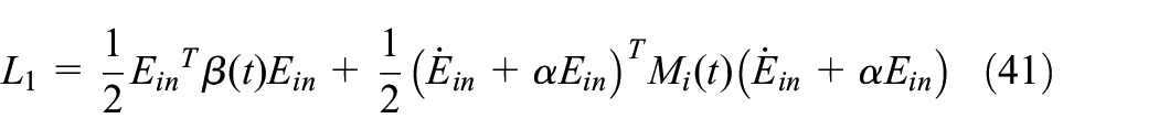
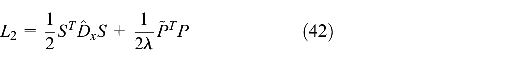
The following amount is offered for the $β (t)$

β (t) = K_{i} (t) + α B_{i} (t) - α^{2} M_{i} (t) - 2 α B_{0} (t)

(45)

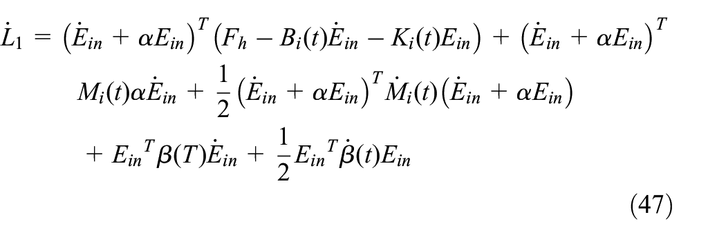
The derivative of Lyapunov function $L_{1}$ is

\begin{matrix} {\overset{\cdot}{L}}_{1} = ({\overset{\cdot}{E}}_{in} + α E_{in})^{T} M_{d} (t) ({\overset{\cdot}{E}}_{in} + α E_{in}) + \frac{1}{2} ({\overset{\cdot}{E}}_{in} + α E_{in})^{T} \\ {\overset{\cdot}{M}}_{d} (t) ({\overset{\cdot}{E}}_{in} + α E_{in}) + \frac{1}{2} {E_{in}}^{T} \overset{\cdot}{β} (t) E_{in} + {E_{in}}^{T} β (t) {\overset{\cdot}{E}}_{in} \end{matrix}

(46)

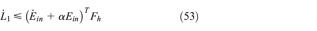
And from equation (28), we get

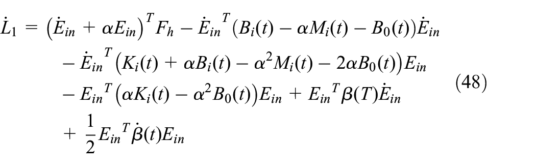
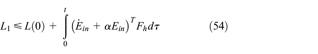
\begin{matrix} {\overset{\cdot}{L}}_{1} = {({\overset{\cdot}{E}}_{in} + α E_{in})}^{T} (F_{h} - B_{i} (t) {\overset{\cdot}{E}}_{in} - K_{i} (t) E_{in}) + {({\overset{\cdot}{E}}_{in} + α E_{in})}^{T} \\ M_{i} (t) α {\overset{\cdot}{E}}_{in} + \frac{1}{2} {({\overset{\cdot}{E}}_{in} + α E_{in})}^{T} {\overset{\cdot}{M}}_{i} (t) ({\overset{\cdot}{E}}_{in} + α E_{in}) \\ + {E_{in}}^{T} β (T) {\overset{\cdot}{E}}_{in} + \frac{1}{2} {E_{in}}^{T} \overset{\cdot}{β} (t) E_{in} \end{matrix}

(47)

Considering equation (44), L₁ converts to

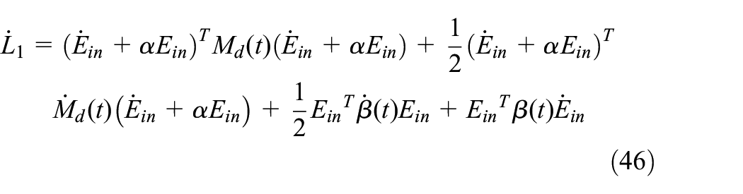
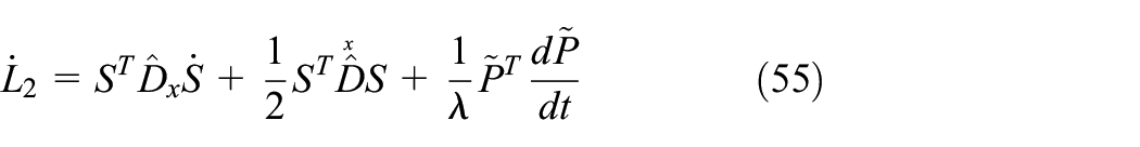
\begin{matrix} {\overset{\cdot}{L}}_{1} = {({\overset{\cdot}{E}}_{in} + α E_{in})}^{T} F_{h} - {\overset{\cdot}{E}}_{in}^{T} (B_{i} (t) - α M_{i} (t) - B_{0} (t)) {\overset{\cdot}{E}}_{in} \\ - {\overset{\cdot}{E}}_{in}^{T} (K_{i} (t) + α B_{i} (t) - α^{2} M_{i} (t) - 2 α B_{0} (t)) E_{in} \\ - {E_{in}}^{T} (α K_{i} (t) - α^{2} B_{0} (t)) E_{in} + {E_{in}}^{T} β (T) {\overset{\cdot}{E}}_{in} \\ + \frac{1}{2} {E_{in}}^{T} \overset{\cdot}{β} (t) E_{in} \end{matrix}

(48)

The derivative of equation (45) is

\dot{β} (t) = {\dot{K}}_{i} (t) + α {\dot{B}}_{i} (t) - α^{2} {\dot{M}}_{i} (t) - 2 α {\dot{B}}_{0} (t)

(49)

From equations (44), (48), and (49), we get

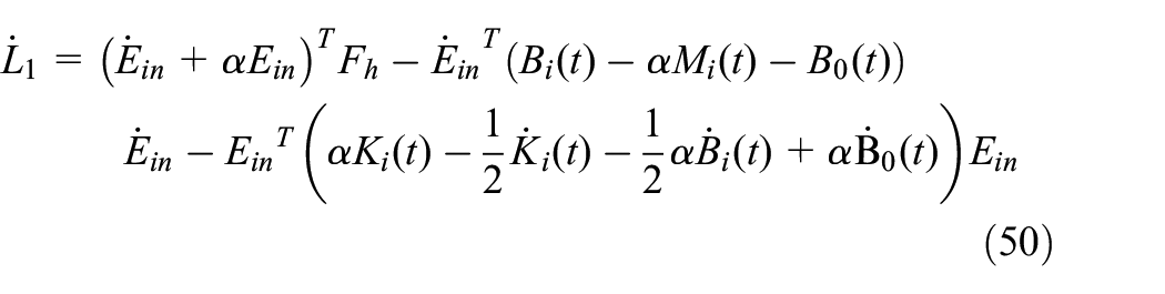
\begin{matrix} {\overset{\cdot}{L}}_{1} = {({\overset{\cdot}{E}}_{in} + α E_{in})}^{T} F_{h} - {\overset{\cdot}{E}}_{in}^{T} (B_{i} (t) - α M_{i} (t) - B_{0} (t)) \\ {\overset{\cdot}{E}}_{in} - {E_{in}}^{T} (α K_{i} (t) - \frac{1}{2} {\overset{\cdot}{K}}_{i} (t) - \frac{1}{2} α {\overset{\cdot}{B}}_{i} (t) + α {\overset{\cdot}{B}}_{0} (t)) E_{in} \end{matrix}

(50)

But for total stability of system, ${\overset{\cdot}{L}}_{1} < 0$ should happen. This function can be evaluated in two phases:

(1)Non-contact phase: in this phase, $F_{h} = 0$ . So equation (50) becomes

\begin{matrix} {\overset{\cdot}{L}}_{1} = - {\overset{\cdot}{E}}_{in}^{T} (B_{i} (t) - a M_{i} (t) - B_{0} (t)) \\ E_{in} - {E_{in}}^{T} (a K_{i} (t) - \frac{1}{2} {\overset{\cdot}{K}}_{i} (t) - \frac{1}{2} a {\overset{\cdot}{B}}_{i} (t) + a {\overset{\cdot}{B}}_{0} (t)) E_{in} \end{matrix}

(51)

In this approach, all coefficients have symmetric, positive definite, and continuously differentiable time-varying matrices, and there always exists a nominal part $B_{0} (t)$ such that, ${\overset{\cdot}{M}}_{i} (t) - 2 B_{0} (t)$ is skew symmetric. In this method, all items should be bounded and a constant amount $α > 0$ , such that ∀ $t \geq 0$ if both below equations are positive semi-definite, ${\overset{\cdot}{L}}_{1} < 0$ will be true (Dong and Ren, 2017)

\begin{matrix} (i) B_{i} (t) - α M_{i} (t) - B_{0} (t) \\ (ii) α K_{i} (t) - (\frac{1}{2}) {\overset{\cdot}{K}}_{i} (t) - (\frac{1}{2}) α {\overset{\cdot}{B}}_{i} (t) + α {\overset{\cdot}{B}}_{0} (t) \end{matrix}

(52)

(2) Contact phase: in this phase, $F_{h} \neq 0$ , if both equations in equation (50) are positive semi-definite,

{\dot{L}}_{1} \leq {({\dot{E}}_{i n} + α E_{i n})}^{T} F_{h}

(53)

The result of above equation is

L_{1} \leq L (0) + \int_{0}^{t} {({\dot{E}}_{i n} + α E_{i n})}^{T} F_{h} d τ

(54)

So if the conditions in equation (52) are positive semi-definite and equation (45) is conducted, $\overset{\cdot}{L_{1}}$ is negative. For the second part of stability proof, we get

{\overset{\cdot}{L}}_{2} = S^{T} {\hat{D}}_{x} \overset{\cdot}{S} + \frac{1}{2} S^{T} \overset{x}{\hat{D}} S + \frac{1}{λ} {\tilde{P}}^{T} \frac{d \tilde{P}}{dt}

(55)

By replacing equation (35) in equation (55), we can write

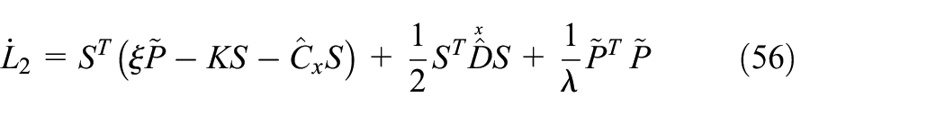
{\dot{L}}_{2} = S^{T} (ξ \tilde{P} - K S - {\hat{C}}_{x} S) + \frac{1}{2} S^{T} \overset{x}{\hat{D}} S + \frac{1}{λ} {\tilde{P}}^{T} \tilde{P}

(56)

According to Assada (2005), we have

\overset{x}{\hat{D}} - 2 {\hat{C}}_{x} = 0

(57)

As a result, equation (56) is given by

{\overset{\cdot}{L}}_{2} = S^{T} ξ \tilde{P} - S^{T} KS + \frac{1}{λ} {\tilde{P}}^{T} \frac{d \tilde{P}}{dt}

(58)

And for having a negative derivative of Lyapunov, the following condition should happen

\frac{d \hat{P}}{dt} = - λ ξ^{T} S

(59)

{\overset{\cdot}{L}}_{2} = - S^{T} KS

(60)

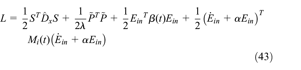
In this way, the centers of fuzzy groups are obtained. It can be seen that the Lyapunov function given by equation (42) is positive and its derivative is in the form of equation (60), which by establishing the relation given by equation (59), the derivative of the Lyapunov function is negative, that is, ${\overset{\cdot}{L}}_{2} < 0$ . Also $P_{l}$ is the center of fuzzy groups and is the outcome of equation (59) and its equation will be updated every cycle with this equation

{\hat{P}}_{1} = - \int_{0}^{t} λ ξ^{T} s d t + {\hat{p}}_{1} (0)

(61)

The $P_{2}$ and $ξ_{2}$ can be gotten in the same equation, $λ$ is positive and is 800. Finally, based on equations (41), (42), (51), (53), and (60), we get

{\overset{\cdot}{L}}_{1} < 0, {\overset{\cdot}{L}}_{2} < 0 \Rightarrow {\overset{\cdot}{L}}_{1} + {\overset{\cdot}{L}}_{2} < 0 \Rightarrow \overset{\cdot}{L} < 0

(62)

L_{1} > 0, L_{2} > 0 \Rightarrow L_{1} + L_{2} > 0 \Rightarrow L > 0

(63)

So based on Lyapunov law, the system is stable and the limits in equation (52) guarantees the safety of the patient.

Physiotherapy training design

For the desired paths, a smooth trajectory is selected, ensuring at least second-order continuity. Furthermore, these paths are constrained within the permissible range of motion for the injured knee or thigh. The training regimen examined in our study focuses on isometric training, serving as a demonstrative example to showcase the controller’s efficacy in generating desired dynamics.

Isometric training involves muscle contraction without accompanying movement in the surrounding joints. This type of exercise emphasizes maintaining constant tension on the muscles, contributing to improvements in muscle endurance and supporting strength training. While many muscle-strengthening exercises entail moving joints and exerting force against resistance, isometric exercises differ by maintaining static positions. In our setup, the joint of the robot coupled to the hip angle is employed for isometric training. Specifically, the robot arm angle initiates from 0 degrees and steadily moves at a constant speed to an angle of 30 degrees in the front position, maintaining this angle thereafter. Similarly, for isometric movement where the knee angle remains constant, the robot arm angle begins at 90 degrees, progressing steadily at a constant speed to an angle of 60 degrees in the front position and maintaining this constant angle throughout.

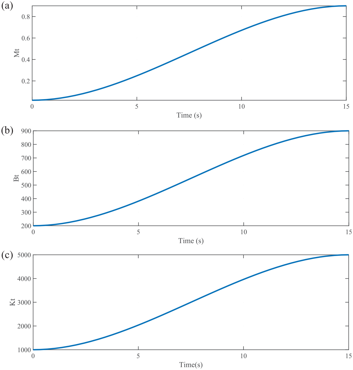
The designed paths for both exercises are represented by third-order equations, satisfying angular boundary conditions. At the initiation and culmination of each path, the angular velocity is set to zero (see Figure 2(a) and (b)). These predetermined paths guide the robot’s end effector to the specified position (see Figure 2(c)) within the task space:

Figure 2.

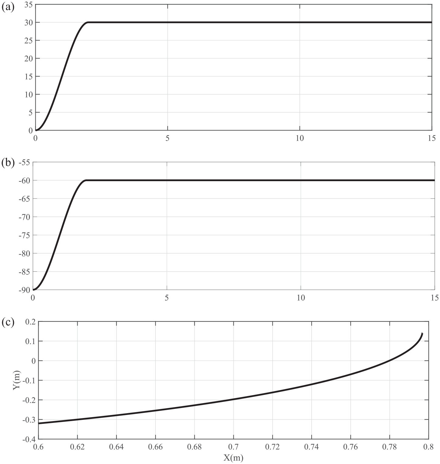
Desired path for the robot: (a) knee joint, (b) hip joint, and (c) end effector.

Yet the time-varying impedance coefficients are the important factors to first, help the joints to have a soft dynamic movement to get the desired constant degree while having the desired dynamic. Second, the constant phase of degree helps the joint to remain constant. These coefficients are designed for the hip as shown below

M_{i} (t) = [\begin{matrix} \frac{- 44}{84375} t^{3} + \frac{22}{1875} t^{2} + \frac{1}{50} & 0 \\ 0 & \frac{- 44}{84375} t^{3} + \frac{22}{1875} t^{2} + \frac{1}{50} \end{matrix}]

(64)

B_{i} (t) = [\begin{matrix} \frac{- 56}{135} t^{3} + \frac{28}{3} t^{2} + 200 & 0 \\ 0 & \frac{- 56}{135} t^{3} + \frac{28}{3} t^{2} + 200 \end{matrix}]

(65)

K_{i} (t) = [\begin{matrix} \frac{- 64}{27} t^{3} + \frac{160}{3} t^{2} + 1000 & 0 \\ 0 & \frac{- 64}{27} t^{3} + \frac{160}{3} t^{2} + 1000 \end{matrix}]

(66)

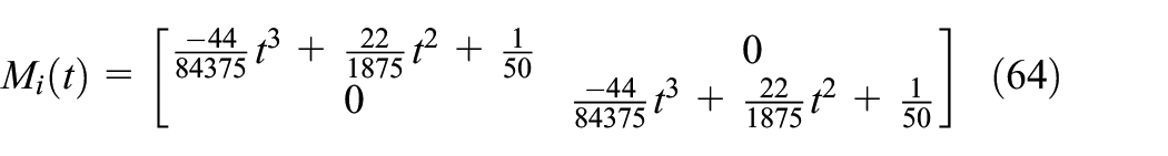
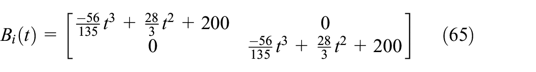
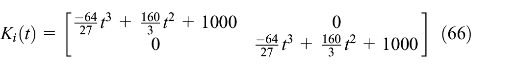
These coefficients are designed to be soft and the patient feels soft in the interaction process. Also when the controller maintains the impedance coefficients in the range of equation (50), the safety of the patient is guaranteed. Also considering the soft amounts for the coefficients during time, this soft rehabilitation causes more natural rehabilitation.

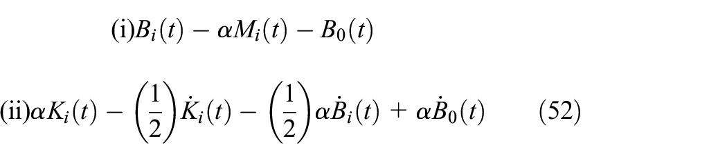
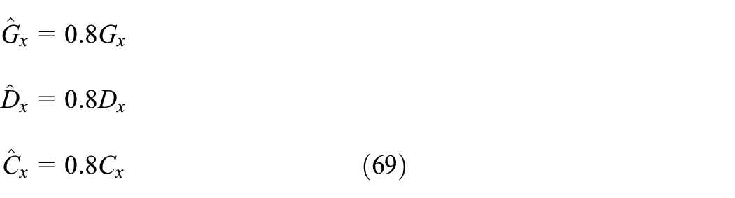
These parameters are designed as an example for showing the capability of the proposed controller for achieving the time-varying dynamics, and every other curve that is helpful for the rehabilitation and satisfies the two limitations for time-varying coefficients (equation (52)) can be utilized. To show these limits in the above example, the first item is $B_{0} (t)$ . ${\overset{\cdot}{M}}_{i} (t) - 2 B_{0} (t)$ is a skew matrix if the $B_{0} (t)$ is a diagonal matrix. So, $B_{0} (t)$ should be selected from diagonal matrixes. In this work, this matrix is

β_{0} (t) = I_{2 \times 2} 5.25

(67)

If equation (52) is formed for the system and $α = 0.1$ , then

\begin{matrix} \begin{matrix} (i) B_{i} (t) - α M_{i} (t) - B_{0} (t) = [\begin{matrix} - 720.0741 t^{3} + 53.3 t^{2} + 194.748 & 0 \\ 0 & - 720.0741 t^{3} + 53.3 t^{2} + 194.748 \end{matrix}] \end{matrix} \\ (ii) α K_{i} (t) - (\frac{1}{2}) {\overset{\cdot}{K}}_{i} (t) - (\frac{1}{2}) α {\overset{\cdot}{B}}_{i} (t) + α {\overset{\cdot}{B}}_{0} (t) = [\begin{matrix} - 0.237 t^{3} + 5.6889 t^{2} - 5.33 t + 100 & 0 \\ 0 & - 0.237 t^{3} + 5.6889 t^{2} - 5.33 t + 100 \end{matrix}] \end{matrix}

(68)

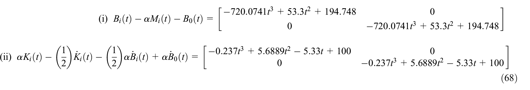
Equation (68) shows that the situation in equation (52) is satisfied. Also, Figure 3 depicts that equations (i) and (ii) are positive. Both above equations (i) and (ii) are positive semi-definite and the selected impedance coefficients are in the stable ranges. Figure 4 depicts that (i) and (ii) are positive.

Figure 3.

The designed impedance coefficients.

Figure 4.

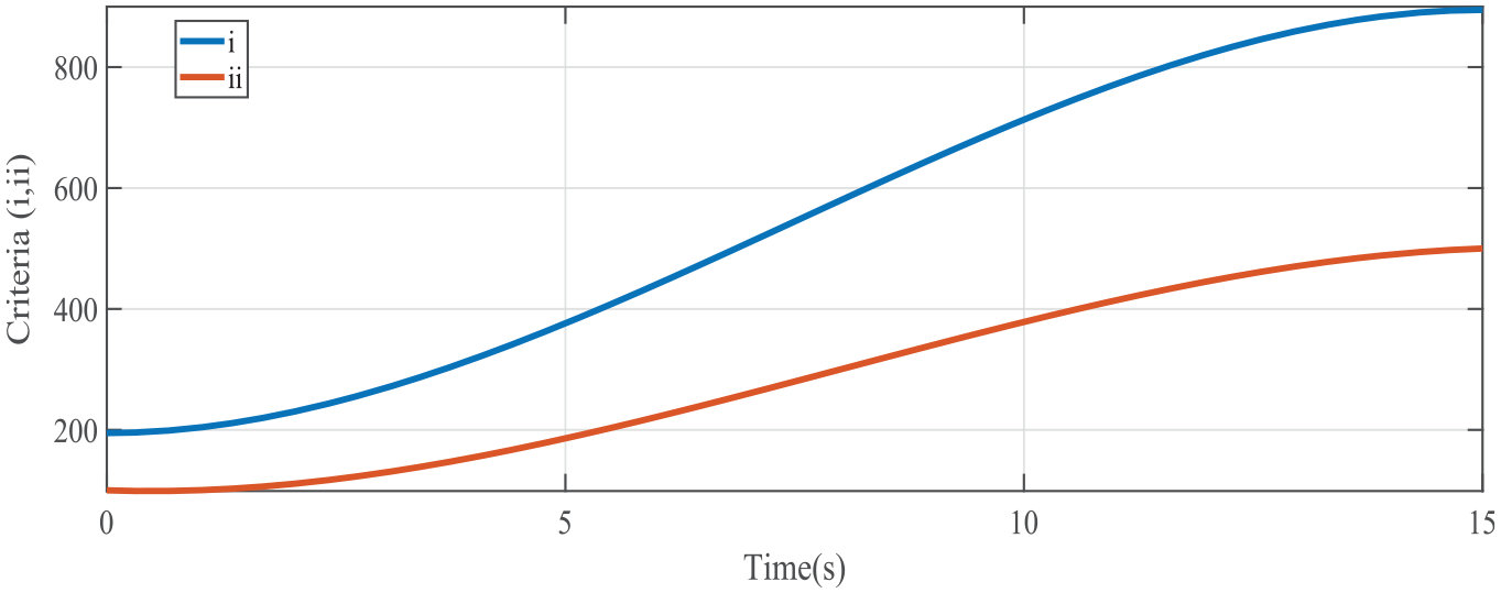
Limitation criteria for time-varying impedance coefficients.

Simulation

In Figure 5, there is the control system of time-varying impedance control.

Figure 5.

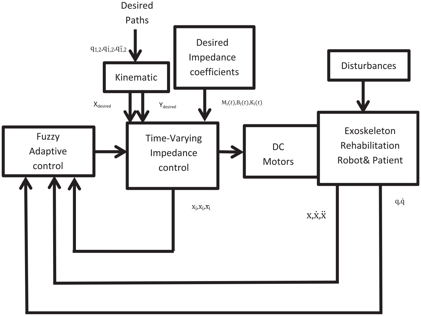
Fuzzy adaptive time-varying impedance control of rehabilitation robot.

For the simulation, the Matlab2023 is used and a rehabilitation robot with two links is used (see Appendix A). The experiment is done for three different patients with different weights (see Table 1) to show the power of the controller for getting the desired impedance.

Table 1.

The weight of limbs of three patients.

Limbs of patient	Hip’s weight (kg)	Knee’s weight (kg)
Patient 1	3	5
Patient 2	5	7
Patient 3	7	9

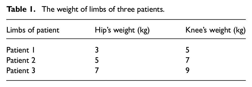
The desired impedance parameters are time-varying and can change the dynamics of the robot and the human during the rehabilitation. The uncertainty is limited and is 20% of the real amount. It means that the model that is used in the controller is 20% or lower than the real model

\begin{matrix} {\hat{G}}_{x} = 0.8 G_{x} \\ {\hat{D}}_{x} = 0.8 D_{x} \\ {\hat{C}}_{x} = 0.8 C_{x} \end{matrix}

(69)

For the disturbance terms, 10% of the input voltage to the actuators is used for simulation of a disturbance. This leads to simulate the disturbance to more natural shape. When the amount of changes of the angle is more the voltage will be more and this leads to more disturbances. This kind of disturbance is near to the disturbances that are related to the patients’ movement. When the motor tries to change the robot’s angle, the patient will move more and this increases the disturbance effect. The parameters of the adaptive fuzzy controller are selected as given below

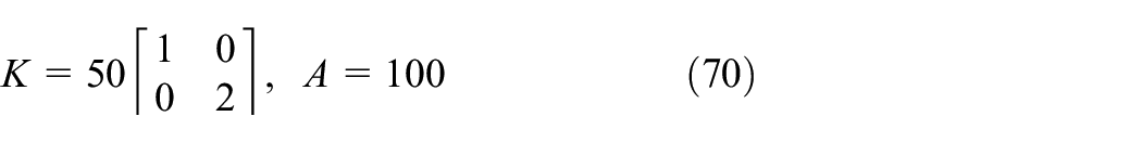
K = 50 [\begin{matrix} 1 & 0 \\ 0 & 2 \end{matrix}], A = 100

(70)

Figure 6 depicts the results of isometric exercise for rehabilitation for time-varying impedance coefficients and constant coefficients. Based on equation (18), the error of the outer layer that is in charge of compensation of uncertainties and disturbances is as given below and shows the difference between x and x_i.

Figure 6.

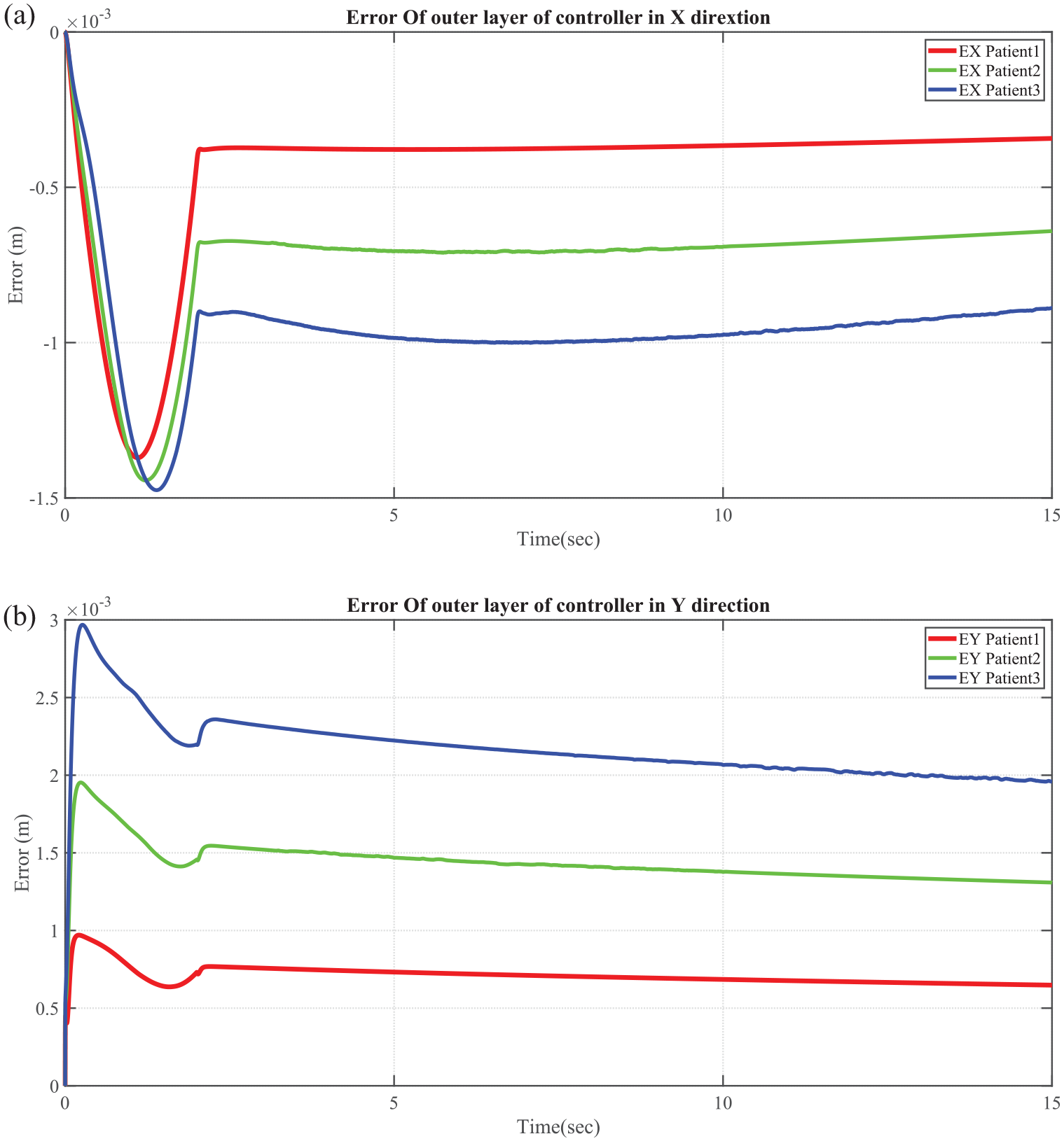
The error of outer layer of controller in X direction. (b) The error of outer layer of controller in Y direction.

This figure illustrates the effective compensation provided by the adaptive fuzzy controller for disturbances and uncertainties, enabling the robot to reach its desired position within the task space for all three patients. Notably, this observation holds true for both time-varying and constant impedance scenarios. Also, the results show that the amount of error for patient 1 in both direction of X and Y is the lowest and for patient 3 the error is the most. This demonstrates that when the weight of the patient increases, the error becomes more but finally for all three patients the amount of error is very low and in patient 3 and in the direction Y, it is 3 mm that is acceptable for the rehabilitation.

It underscores the adaptive fuzzy controller’s ability to mitigate the impact of disturbances and uncertainties independently of the inner control layer. Given that the inner controller effectively manages the system to attain the desired dynamics, achieving the desired impedance becomes feasible. In this study, particular emphasis is placed on voltage control. By manipulating the motors’ voltage, the system can be steered toward the desired dynamics as shown in Figure 7.

Figure 7.

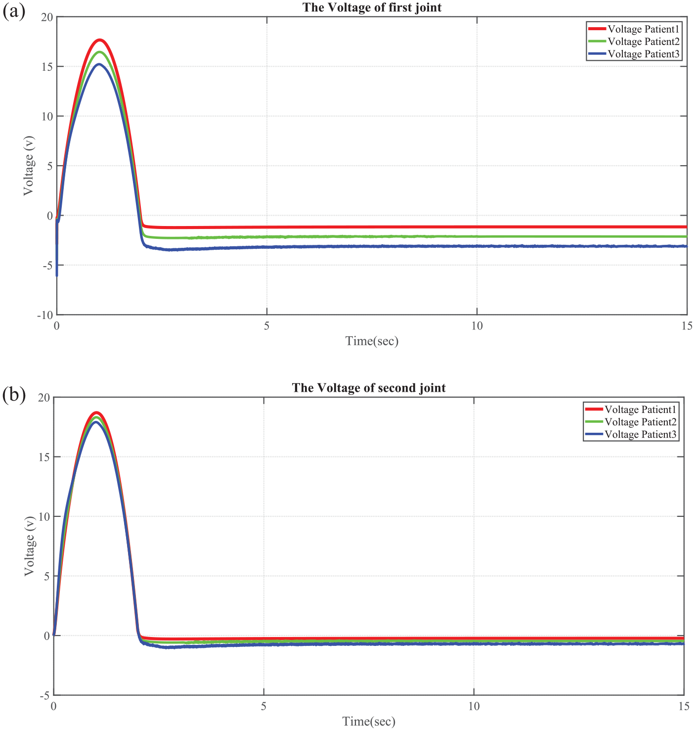
The voltage of the first and second joint for all patients.

The voltages depict that between 0 and 2 seconds, the voltage increases to get the desired task space trajectory, then the voltage remains stable to robots linkages that have constant degrees. The voltages are the outer layer output of the controller. Obviously for the third patient that have heavier limbs, the amount of voltage for tracking the time-varying impedance increases more and when the limbs get the desired impedance the voltage of the first patient becomes less than the other two. This phenomenon is because of more control attempt by the controller for the heavier person.

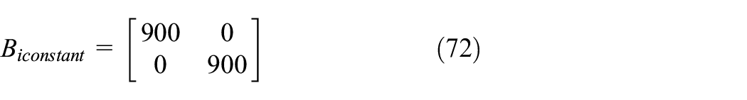
Now for a better understanding of the efficiency of time-varying impedance, we compare the results of time-varying impedance with the constant impedance control. In the same situation that all control coefficients of control like $K$ and $A$ are the same, when the coefficients of impedance do have not the possibility of increase and are constant, the results can demonstrate the good effectiveness of time-varying impedance. In this case, we suppose that the impedance coefficients of impedance are

M_{iconstant} = [\begin{matrix} 1 & 0 \\ 0 & 1 \end{matrix}]

(71)

B_{iconstant} = [\begin{matrix} 900 & 0 \\ 0 & 900 \end{matrix}]

(72)

K_{iconstant} = [\begin{matrix} 5000 & 0 \\ 0 & 5000 \end{matrix}]

(73)

These are the exact amount of impedance coefficients that the time-varying impedance coefficients had at the final of the path. The output trajectory that leads the x_i to track the x_d and causes the system to have the desired dynamic known in this paper as the E_in is shown in Figure 8.

Figure 8.

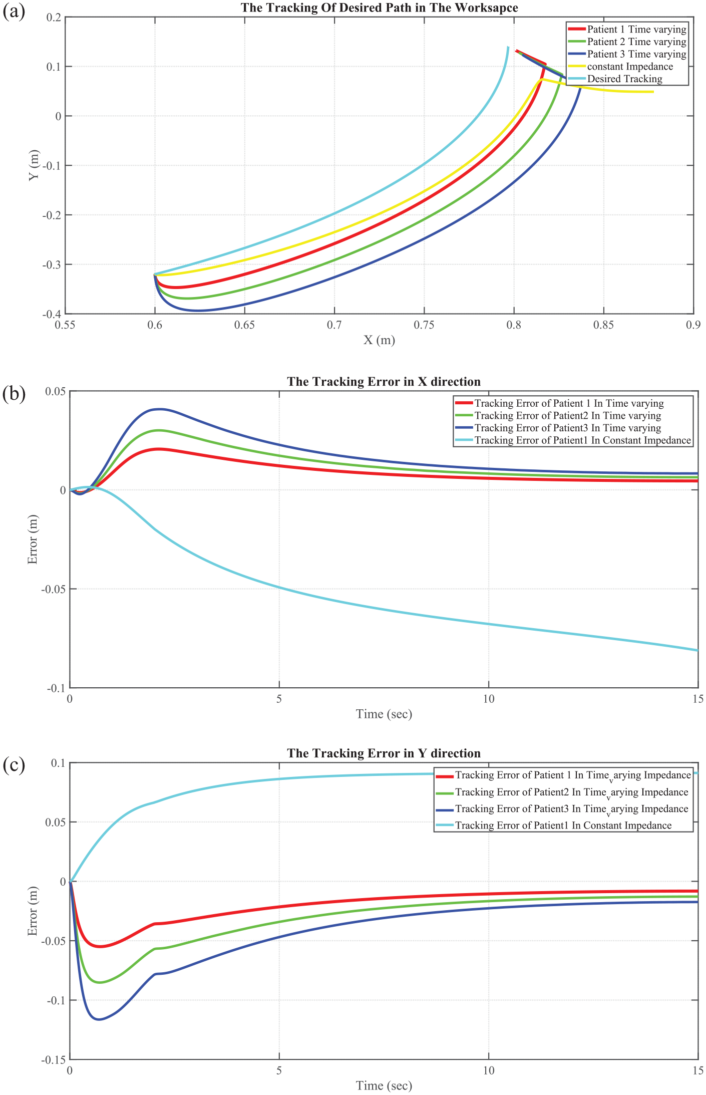
(a) Results of trajectory in task space, (b) error of tracking in x direction, and (c) error of tracking in y direction.

The results depict that the time-varying impedance control has better results for tracking a path and this is added to the main goal of this research which is having the desired dynamic with time-varying impedance coefficients. The results show that error of impedance in the X and Y direction are the most for patient 3, that is the biggest patient and the robot faced the more disorientation in comparison to the patient 1. But in the case of the constant impedance even while patient 1 is under the experiment the steady error in the Y and X direction is twice the heaviest patient (3) in the time-varying impedance. On the contrary, the constant coefficients that kept the primary amounts of impedance coefficients had the worst results in comparison to the time-varying impedance. The norm of error in task space for n sample in time is

E_{norm} = \frac{1}{n} \sum_{i = 1}^{n} \sqrt{({E_{x_i}}^{2} + {E_{y_i}}^{2})}

(74)

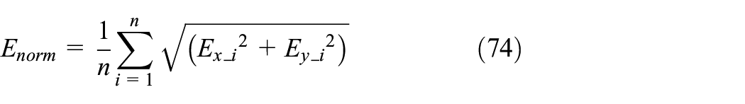
This criterion is compared for the constant and time-varying impedance control and is the norm of error in the task space and for time-varying impedance with 10,547 samples is 0.0320 and for constant impedance with 45,372 samples is 0.0505. These data prove that the error of tracking in the time-varying impedance is less than the constant impedance and the ability to change during time helps the time-varying impedance to decrease the error and get the desired dynamic at the same time. Finally, the goal of isometric rehabilitation exercise is to have a constant force in the end effector of the exoskeleton robot to make the muscles of the patient stronger. This force is made by the impedance control and is shown in Figure 9.

Figure 9.

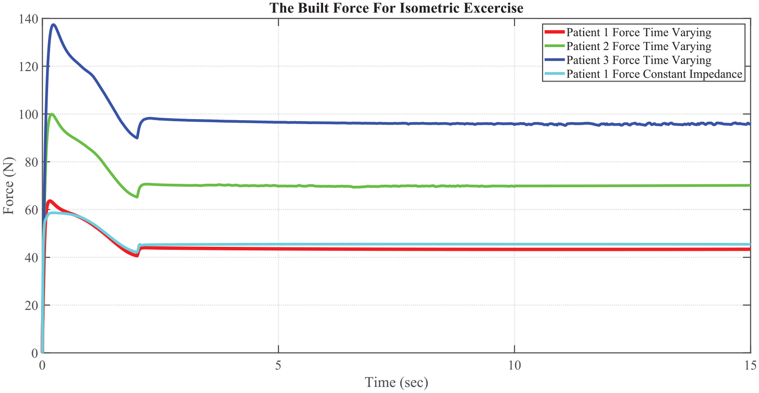
The produced force by the exoskeleton robot for the patient in the isometric exercise.

Based on this figure, both constant and time-varying impedance controllers are able to produce a constant force for the end effector of the robot and time-varying impedance has less amount of force and this is because of less trajectory, velocity, and acceleration error in equation (27) that make the force for the end effector. This less force is not as important as imitating the desired time-varying dynamic and less tracking error. As the impedance coefficients are the same for all patients in the time-varying experiment, patient 3 that is the heaviest patient faces the most force that is 100 N in the stable condition and patient 2 endures the force 80 N in the stable condition. The happening is adapted to the need of the different patients that based on the volume of their muscles, they should have various forces. By knowing the best fit of dynamic that has the best performance for the rehabilitation, the exoskeleton robot can follow this dynamic behavior and get the desired dynamic even with the disturbances and uncertainties.

Conclusion and future research

This research is concerned with providing the best rehabilitation exercise for patients by using an exoskeleton robot for the knee and hip. The controller has two loops; in the outer loop, the fuzzy adaptive controller is used to achieve the current position of the robot in the task space to the x_i which is known as the impedance state. The inner control loop is used to change the dynamic of the robot and patient to the desired dynamic, which is a time-varying dynamic, and uses the impedance coefficients to change the dynamical model. The Lyapunov method is used to show the stability of the system. All of the impedance coefficients are time-varying, which are important matters in comparison to the previous works. The limits of these coefficients are determined by the Lyapunov theory and the adaptive fuzzy controller could handle the system while there are disturbances in the system and there are uncertainties in all terms of robots and patients. The results depict that the time-varying impedance controller has a good performance to get the desired trajectory and can change the dynamic of the robot well while producing the force for the isometric exercise. This feature can be used in all exoskeleton robots to change the dynamic of the system to the best dynamic that can satisfy the best performance for the robot while having a stable and safe interaction with humans.

For future works, it is recommended to use neural networks and other functions to get the best dynamic of the rehabilitation. This matter can be done by using a professional rehabilitation expert and taking the data of the dynamic movements of this person. Then by utilizing detection methods like fuzzy and neural networks, these dynamics can be found and the time-varying coefficients with stable limitations that are as same as our work can be detected. The next step that can be done is using the CBFs (control barrier functions) to have safe interaction during the rehabilitation process that is less worked and known.

Footnotes

Appendix A

The two-links robot has a dynamic model that is

(75)

D (q) \overset{\cdot\cdot}{q} + C (q, \overset{\cdot}{q}) \overset{\cdot}{q} + G (q) - J^{T} (q) F_{h} = τ_{r}

$D$ is inertia of robot and is given as

(76)

D = [\begin{matrix} d_{11} & d_{12} \\ d_{21} & d_{22} \end{matrix}]

where

(77)

\begin{matrix} d_{11} = m_{1} l_{c 1}^{2} + I_{1} + m_{2} (l_{1}^{2} + l_{c 2}^{2} + 2 l_{1} l_{c 2} \cos q_{2}) + I_{2} \\ d_{21} = d_{12} = m_{2} (l_{c 2}^{2} + l_{1} l_{c 2} \cos q_{2}) + I_{2} \\ d_{22} = m_{2} (l_{c 2}^{2}) + I_{2} \end{matrix}

In these equations, $m_{1}$ and $m_{2}$ are, respectively, mass of first and second links; $I_{1}$ and $I_{2}$ are inertia of first and second links; $l_{1}, l_{2}, l_{c 2}$ are the length of first and second link and the location of the center of mass of the second interface; $q_{1}$ and $q_{2}$ are the degree between the first and second links. $C$ is the vector of centrifugal and Coriolis torques of the robot and is given by

(78)

C = [\begin{matrix} c_{11} & c_{12} \\ c_{21} & c_{22} \end{matrix}]

where

(79)

\begin{matrix} c_{11} = - 2 l_{1} l_{c 2} m_{2} \sin (q_{2}) {\overset{\cdot}{q}}_{2} \\ c_{12} = - l_{1} l_{c 2} m_{2} \sin (q_{2}) {\overset{\cdot}{q}}_{2} \\ c_{21} = l_{1} l_{c 2} m_{2} \sin (q_{2}) {\overset{\cdot}{q}}_{1} \\ c_{22} = 0 \end{matrix}

In this equation, ${\overset{\cdot}{q}}_{1}$ and ${\overset{\cdot}{q}}_{2}$ are the angular velocity of the interface in the first and second. Also, the matrix $G$ is $1 \times 2$ and represents the vector of gravitational moments and is displayed as follows

(80)

G = [\begin{matrix} g_{1} \\ g_{2} \end{matrix}]

where

(81)

\begin{matrix} g_{1} = g (m_{1} l_{c 1} \cos (q_{1}) + m_{2} (l_{1} \cos (q_{1}) + l_{c 2} \cos (q_{1} + q_{2}))) \\ g_{2} = g (m_{2} l_{c 2} \cos (q_{1} + q_{2})) \end{matrix}

In the above equations, g is the acceleration of the center of the earth and is equal to 9.81 meters per square second. Also, the Jacobian matrix of the robot is as follows

(82)

J_{e} = [\begin{matrix} j_{11} & j_{12} \\ j_{21} & j_{22} \end{matrix}]

where

(83)

\begin{matrix} j_{11} = - l_{1} \sin (q_{1}) - l_{c 2} \sin (q_{1} + q_{2}) \\ j_{12} = - l_{c 2} \sin (q_{1} + q_{2}) \\ j_{21} = l_{1} \cos (q_{1}) + l_{c 2} \cos (q_{1} + q_{2}) \\ j_{22} = l_{c 2} \cos (q_{1} + q_{2}) \end{matrix}

Declaration of conflicting interests

The author(s) declared no potential conflicts of interest with respect to the research, authorship, and/or publication of this article.

Funding

The author(s) received no financial support for the research, authorship, and/or publication of this article.

ORCID iDs

Sayed Reza Mohamadi

Saeed Khorashadizadeh

Data availability statement

The results are obtained by computer simulations of dynamical systems and no dataset has been used.

References

Ajoudani

Tsagarakis

Bicchi

(2012) Tele-impedance: Teleoperation with impedance regulation using a body–machine interface. The International Journal of Robotics Research 31: 1642–1656.

Akdogan

Arif

(2011) The design and control of a therapeutic exercise robot for lower limb rehabilitation: Physiotherabot. Mechatronics 21: 509–522.

Burdet

Ganesh

Yang

, et al. (2014) Interaction force, impedance and trajectory adaptation: By humans, for robots. In: Sukhatme

Khatib

Kumar

(eds) The 12th International Symposium on Experimental Robotics. Berlin and Heidelberg: Springer, pp. 331–345.

Chien

Huang

(2004) Adaptive impedance control of robot manipulators based on function approximation technique. Robotica 22(4): 395–403.

Dong

Ren

(2017) UDE-based variable impedance control of uncertain robot systems. IEEE Transactions on Systems, Man, and Cybernetics: Systems 49(12): 2487–2498.

Farahat

Herr

(2010) Optimal workloop energetics of muscle-actuated systems: An impedance matching view. PLoS Computational Biology 6(6): e1000795.

Fateh

Khoshdel

(2015) Voltage-based adaptive impedance force control for a lower-limb rehabilitation robot. Advanced Robotics 29(15): 961–971.

Ferraguti

Secchi

Fantuzzi

(2013) A tank-based approach to impedance control with variable stiffness. In: 2013 IEEE international conference on robotics and automation, Karlsruhe, 6–10 May, pp. 4948–4953. New York: IEEE.

Ficuciello

Villani

Siciliano

(2015) Variable impedance control of redundant manipulators for intuitive human–Robot physical interaction. IEEE Transactions on Robotics 31(4): 850–863.

10.

Furui

Nakagaki

Tsuji

(2021) Biomimetic control of myoelectric prosthetic hand based on a lambda-type muscle model. In: 2021 IEEE international conference on robotics and automation (ICRA), Xi’an, China, 30 May–5 June, pp. 10484–10490. New York: IEEE.

11.

Hamedani

Zekri

Sheikholeslam

, et al. (2021) Recurrent fuzzy wavelet neural network variable impedance control of robotic manipulators with fuzzy gain dynamic surface in an unknown varied environment. Fuzzy Sets and Systems 416: 1–26.

12.

Huang

Chen

(1992) Compliant motion control of robots by using variable impedance. The International Journal of Advanced Manufacturing Technology 7(6): 322–332.

13.

Ikeura

Moriguchi

Mizutani

(2002) Optimal variable impedance control for a robot and its application to lifting an object with a human. In: 11th IEEE international workshop on robot and human interactive communication, Berlin, 27 September, pp. 500–505. New York: IEEE.

14.

Jin

Guo

(2023) Disturbance rejection model predictive control of lower limb rehabilitation exoskeleton. Scientific Reports 13(1): 19463.

15.

Kim

(2016) Position-based impedance control for force tracking of a wall-cleaning unit. International Journal of Precision Engineering and Manufacturing 17(3): 323–329.

16.

Kronander

Billard

(2016) Stability considerations for variable impedance control. IEEE Transactions on Robotics 32(5): 1298–1305.

17.

Lee

Buss

(2008) Force tracking impedance control with variable target stiffness. In: 17th IFAC world congress, Seoul, Korea, 6–11 July, pp. 6751–6756. Laxenburg: International Federation of Automatic Control.

18.

Ganesh

Jarrassé

, et al. (2018) Force, impedance, and trajectory learning for contact tooling and haptic identification. IEEE Transactions on Robotics 34(5): 1170–1182.

19.

Huang

, et al. (2016) Adaptive impedance control for an upper limb robotic exoskeleton using biological signals. IEEE Transactions on Industrial Electronics 64(2): 1664–1674.

20.

Liang

Yang

Wang

, et al. (2014) Implementation and test of human-operated and human-like adaptive impedance controls on baxter robot. In: 15th annual conference on advances in autonomous robotics systems, Birmingham, 1–3 September, pp. 109–119. Sheffield: TAROS.

21.

Liang

Zhang

, et al. (2022) An adaptive time-varying impedance controller for manipulators. Frontiers in Neurorobotics 16: 789842.

22.

Mersha

Stramigioli

Carloni

(2014) Variable impedance control for aerial interaction. In: 2014 IEEE/RSJ international conference on intelligent robots and systems, Chicago, IL, 14–18 September, pp. 3435–3440. New York: IEEE.

23.

Muller

Janetzky

Behrnd

, et al. (2018) User force-dependent variable impedance control in human-robot interaction. In: 14th international conference on automation science and engineering (CASE), Munich, 20–24 August, pp. 1328–1335. New York: IEEE.

24.

Oguztöreli

Stein

(1991) The effect of variable mechanical impedance on the control of antagonistic muscles. Biological Cybernetics 66: 87–93.

25.

Park

Lee

(2004) Adaptive impedance control of a haptic interface. Mechatronics 14(3): 237–253.

26.

Sharifi

Behzadipour

Vossoughi

(2014) Nonlinear model reference adaptive impedance control for human–robot interactions. Control Engineering Practice 32: 9–27.

27.

Sun

Peng

Cheng

, et al. (2019) Stability-guaranteed variable impedance control of robots based on approximate dynamic inversion. IEEE Transactions on Systems, Man, and Cybernetics: Systems 51(7): 4193–4200.

28.

Tsumugiwa

Yokogawa

Hara

(2002) Variable impedance control based on estimation of human arm stiffness for human-robot cooperative calligraphic task. In: IEEE international conference on robotics and automation, Washington, DC, 11–15 May, pp. 644–650. New York: IEEE.

29.

Yang

Ganesh

Haddadin

, et al. (2011) Human-like adaptation of force and impedance in stable and unstable interactions. IEEE Transactions on Robotics 27(5): 918–930.

30.

Zheng

Yuan

Huang

(2018) Time-varying impedance control of port Hamiltonian system with a new energy-storing tank. Complexity 2018: 8134230.