The development of an analytical method for constructing noise contours

Abstract

Noise is one of the most pervasive occupational health problems. Noise contours provide useful information by clearly identifying areas where noise hazards exist. This study finds an efficient algorithm for computing sound level in industrial buildings that accounts for reverberation effects. This study proposes an analytical image method to calculate workplace noise distribution by using machinery noise labeling. Contours are then obtained by joining locations with equal noise levels using commercially available software. To demonstrate the application of the proposed method, a manufacturing plant building is considered. The computation algorithm accounts for distance and sound reflection to construct noise contours. The proposed approach could be used in industry for noise management when designing new plant buildings and installing machines.

Practical applications: Machine noise emission information will be widely used in practice to evaluate the potential and performance of noise levels in industrial buildings. Plant buildings should be designed to prevent or minimize any risks to health or safety resulting from the emission of noise. The construction of noise contours will have direct implications for the hearing conservation program.

Keywords

Building acoustics image method noise map hearing loss

Introduction

Noise is one of the most pervasive occupational health problems in industrial facilities. A review of the literature indicates that noise has several health effects, including hearing impairment.¹ Some of these, such as sleep deprivation, are important for environmental noise control,² but are less likely to be associated with workplace noise. Other consequences of workplace noise, such as annoyance, hypertension, disturbance of psychosocial well-being, and psychiatric disorders, have also been described.^3–6 Measuring noise levels and worker noise exposure is the most important part of a workplace hearing conservation and noise control program.⁷ It is also a legal requirement if an employee is exposed to noise that exceeds the noise exposure standard. Noise surveys should be conducted in areas where noise exposure is likely to be hazardous. Noise maps provide useful information by clearly identifying areas where noise hazards exist and may be used to show workers the degree of noise hazard in their work areas, as an easy-to-understand educational tool during management presentations, to identify dominant noise sources in a work area or to identify high noise locations close to dominant noise sources, and to approximate employee noise exposure. Traditionally, noise mapping takes measurements at predetermined positions identified by applying an approximately 3-m grid to the floor plan. When the observed noise levels vary significantly, then a smaller grid pattern will be necessary. These measurements are then displayed on the floor plan to produce a contour map.

Despite national regulations on workplace noise, many people still experience hearing loss from machinery noise in Europe. A need existed for policy at the design stage to enforce noise reduction at source and to allow market forces to encourage the development of less noisy machinery. Many European Directives, such as Directive 89/392/EEC (1989), Directive 2000/14/EC (2000), and Directive 2006/42/EC (2006)^8–10 contain requirements for determining machine sound power levels. The Control of Noise at Work Regulations (HSE 2005)¹¹ require suppliers of machines or equipment for use in factories to provide information on noise levels emitted and label machines if they are likely to expose workers to excessive noise. Sound power level information should also be provided. Sound power is the rate at which a source radiates sound energy and is independent of all other factors, including the environment in which the source is located. Sound pressure level is the acoustic disturbance produced at a point and must always be specified at a position, such as the distance from the source, or in a particular environment. An advantage of sound power level is that the data can be used in acoustic calculations, for example, to predict likely noise levels while planning a new installation, and to plan a proper layout of all these machines and equipment in their workplace. A computer model would enable an employer to rearrange the working environment or an architect to design an industrial unit meeting the legislation, if necessary by the application of noise control measures.

The physical phenomena involved in sound wave propagation inside enclosures are numerous and complex, making overall analytical modeling difficult. Because many parameters must be accounted for when describing a real situation, only an approximation of reality is possible.¹² Inside a room or a similar enclosed space, sound is reflected off surfaces depending on their acoustic absorbent properties. Calculations of the sound pressure level at any point must account for directly radiated and reflected sound. Direct sound energy depends on the source directivity factor and the source-receiver distance. The reverberant sound field, by contrast, is usually considered uniform throughout the room which does not usually occur in real rooms. Practitioners use diffuse field theory to predict sound fields in rooms of all types, but they often forget that the theory is based on assumptions which limit its applicability. If theoretical assumptions do not apply to a particular room, predictions may be inaccurate.^13,14 For instance, diffuse field theory cannot be applied in highly absorptive rooms. Cotana,¹⁵ Hodgon,^14,16 Kuttruff,¹⁷ and Thompson et al.³ have proposed other methods and refinements; however, these methods use other approximations and limitations and have not been proven efficient in various enclosures. Even if a room constant is introduced to include the contribution of reverberant sound energy, this can be theoretically calculated from the acoustic absorption coefficients and areas of the different materials in the space.^18,19 In practice, the room constant is often calculated from the reverberation time which has been measured experimentally. Only radiation under free field conditions is considered to analytically construct noise contours.²⁰

Reasonably accurate commercial ray-tracing and finite element method modeling programs are available. Many previous studies used ray tracing rather than an image model. Ray tracing tends to be easier to program, particularly when dealing with complex geometries. Although both approaches are based on the same assumptions of geometrical acoustics, they mechanize the analysis differently. In ray tracing, the source is assumed to emit a finite number of sound rays in many directions. These rays are extended by linear extrapolation and reflection until they reach a zone of space surrounding the listener. Unfortunately, ray tracing will not find all the sound paths whose length is less than a given amount. Computer modelling has been used to predict sound distribution in factory spaces during the past decades; the room acoustics software, such as ODEON, CadnaR, CATT, etc. have emerged as the powerful tool for simulating the interior acoustics of buildings. The two disadvantages of the commercial software are the runtime requirements and the extensive information necessary to represent an enclosed space. However, creating a model and performing calculations are time-consuming and their use in preliminary room acoustic design is not always cost-effective. These sophisticated room acoustic modeling programs demand special expertise which limits their practical use. The image model is a technique that is widely known for analyzing the acoustical properties of a space that includes reflecting boundaries. When this idea is applied to a rectangular room, the calculation of the image positions is trivial.^21,22 But real industrial plants may not be perfectly rectangular, so accurate modeling requires that the image model be generalized. For irregular shapes, it is more difficult to find the image positions. Moreover, it is necessary to consider in irregular shapes that a sound source might not contribute reflected sound to every position in the plant. The extension of the image model presented in the current study makes it possible to deal with polyhedral room having any number of sides. The following describes a methodology that is simple, easy to use, and fast for computing the image positions in a polygonal room with an arbitrary shape, and also some preliminary results of applying this methodology.

Methods

The concept of the image model is simple and is represented in two dimensions in Figure 1, which shows the concept for the image sources distributed over the x–y plane. It is based on the principle that a specular reflection can be geometrically constructed by mirroring the source in the plane of the reflecting surface. In the image method, direct paths from reflected mirror images of the source replace reflected paths from the real source. Sound source S is mirrored on the other side of each surface, creating S′ image sources, for example, through wall i and $S'_{i}$ , i = 1 … 5. The reflected path is then replaced by a virtual path that goes from the image source to receiver location R.

Figure 1.

Cross-section of the x–y plane of an image source model of a chamber with five reflecting walls.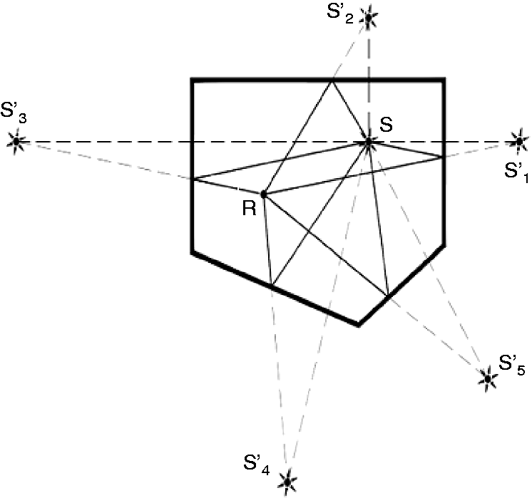

Finding the coordinates of image sources

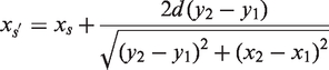
Given a wall (reflecting plane) with an arbitrary orientation and a point source, an expression for the position of the image source must be located. The unit vector normal to plane $n$ describes the orientation of the reflecting plane. In Figure 2, the position of the image source is found by traveling distance 2d from the real source in the direction of unit vector $n$ . Therefore, the position vector of the image source is

O S^{'} = OS + 2 d \cdot n .

Figure 2.

Diagram showing how to determine the image source position.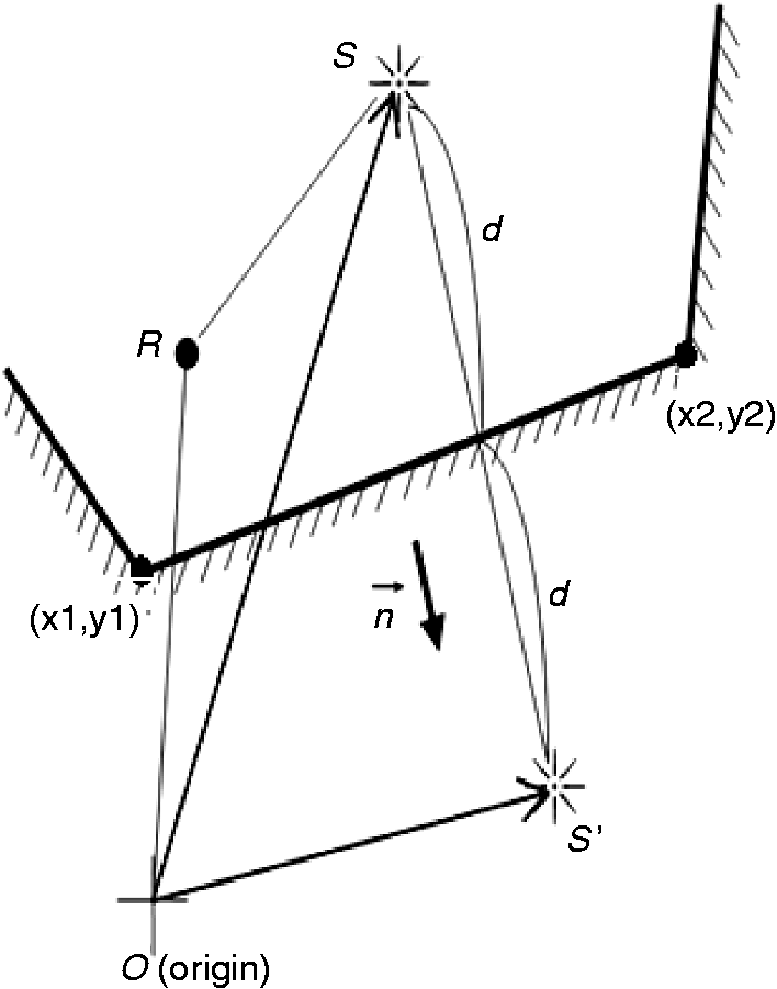

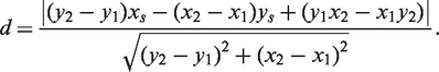
Assuming a room with a high ceiling, consider the two-dimensional problem. The source coordinate is (x_s, y_s) and the end coordinates of the reflecting side are (x₁, y₁) and (x₂, y₂). The distance d from the source to the reflecting side is calculated by

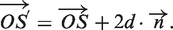
d = \frac{| (y_{2} - y_{1}) x_{s} - (x_{2} - x_{1}) y_{s} + (y_{1} x_{2} - x_{1} y_{2}) |}{\sqrt{{(y_{2} - y_{1})}^{2} + {(x_{2} - x_{1})}^{2}}} .

Vector $O S'$ from the image source to the room receiver has components calculated using

x_{s^{'}} = x_{s} + \frac{2 d (y_{2} - y_{1})}{\sqrt{{(y_{2} - y_{1})}^{2} + {(x_{2} - x_{1})}^{2}}}

(1a)

y_{s^{'}} = y_{s} + \frac{2 d (x_{2} - x_{1})}{\sqrt{{(y_{2} - y_{1})}^{2} + {(x_{2} - x_{1})}^{2}}}

(1b)

Performing the image source visibility test

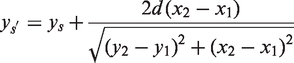
The purpose of the visibility test is to determine which image sources contribute reflected sound to the room positions. As shown in Figure 3, when obtuse angles exist, the receiver may not be able to “see” the image source. An image source may not be “visible” from every room position and a visibility test must be performed to determine which image sources are visible. A simple method of testing for visibility is described as follows. Three vectors are formed, each joining the image source with receiver $S^{‘} R$ and the two end points of reflecting plane line $S^{’} A$ , $S B$ . The cross products of vector pairs $S^{'} R \times S' A$ and $S^{'} R \times S' B$ are in the same direction if receiver R is located in the invisible region shown in Figure 3. Otherwise, receiver R is inside the visible region and the image source is visible.

Figure 3.

The receiver must be in the grid region for image source S′ created by side AB to be visible.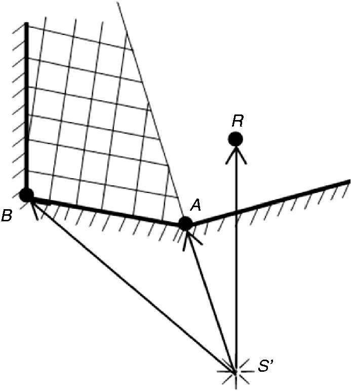

Predicting the sound pressure level inside a room

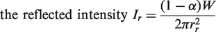
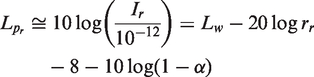
Assume a sound source of power W is located on the ground and placed near a reflecting surface. An image source results with power (1-α) W, where α is the absorption coefficient of the surface. For a sound source in a room, the sound pressure level is the sum of the direct and reverberant sound. The propagation path of the reflected ray is equal to the line from the image source to the receiving point. Therefore, the sound intensity (I) for a receiver is expressed as follow

I = I_{d} + I_{r}

(2)

and the direct intensity I_{d} = \frac{W}{2 π r_{d}^{2}}

(3)

the reflected intensity I_{r} = \frac{(1 - α) W}{2 π r_{r}^{2}}

(4)

where W is sound power in watts; and

r_{d}

and

r_{r}

are the distance of the direct path and reflected path, respectively.

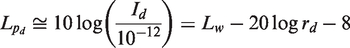
The sound pressure levels of direct sound ( $L_{p_{d}}$ ) and reverberant sound ( $L_{p_{r}}$ ) within the room are approximated using

L_{p_{d}} ≅ 10 \log (\frac{I_{d}}{10^{- 12}}) = L_{w} - 20 \log r_{d} - 8

(5)

and

L_{p_{r}} ≅ 10 \log (\frac{I_{r}}{10^{- 12}}) = L_{w} - 20 \log r_{r} - 8 - 10 \log (1 - α)

(6)

where

L_{w}

is the sound power level of the source in decibels (dB) re picowatt (pW).

When multiple sources and multiple reflecting surfaces in a room are considered, the total sound pressure level (L_pt) of each receiving position is calculated as follow

L_{pt} = 10 \log (\sum_{i = 1}^{m} 10^{L_{p di} / 10} + \sum_{j = 1}^{n} 10^{L_{p rj} / 10}) = 10 \log (\sum_{i = 1}^{m} 10^{(L_{w_{i}} - 20 \log r_{d_{i}} - 8) / / 10} + \sum_{j = 1}^{n} 10^{(L_{w_{j}} - 20 \log r_{r_{j}} - 8) / 10})

(7)

where m is the number of sound sources and n is the number of visible image sources.

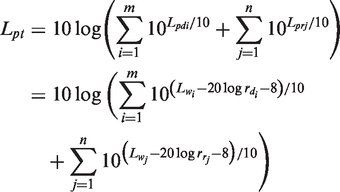
The calculations from these simple equations are quick and it is easy to add the image source contributions to the sound field at a receiver point. Although the number of images is theoretically infinite, it is possible to only consider the contribution of first order images that are generated.

Numerical example

To demonstrate the application of the proposed method, consider a manufacturing plant production room. The concrete construction room with painted cement walls is 2 100 cm (length) × 800 cm (width) × 1 000 cm (height) and the absorption coefficient (α = 0.01–0.03) of the reflecting wall is negligible. Assuming that the reference origin is in the lower left corner of the layout map, the machine location is expressed as a pair of x and y coordinates which are measured from the reference origin. There are three machines (noise sources), with sound power levels of 97.8 dB, 88.7 dB, and 88.1 dB re 1 picowatt, located at positions (420, 1 110), (60, 1 740), and (60, 1 650), respectively. Figure 4 shows the layout of the room. The plant layout map is initially divided into grids. The grid dimensions used are 90 cm × 60 cm (length × width). At each grid corner, the combined noise level is computed as follows. First, locate the coordinates of 12 image sources (three real sources × four reflecting walls) using (1a) and (1b). Visibility testing shows that all image sources are visible from every position (receiver) in the room because there are no obtuse angles. Second, calculate the distances between each grid corner and source, including real and image sources. Third, combine the direct sound level and reflected sound level using (7) to obtain total sound pressure level L_pt at each grid corner.

Figure 4.

Floor layout of the production room (the figure is not drawn to scale).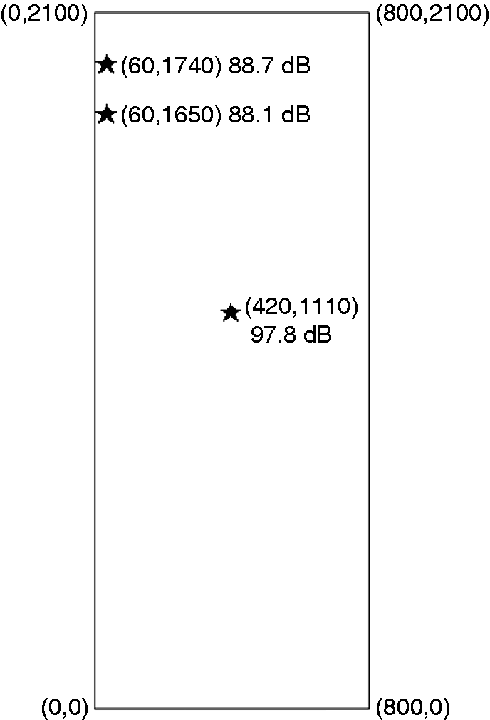

Commercially available software and the calculated results are used to obtain the noise contour map showing noise distribution in the room (Figure 5). The curves show that, at a point close to the source, the direct sound level contributes the most to the total sound level. Further from the source, the relative contribution of the direct sound level decreases and the total sound pressure level decreases, approaching the reflected sound pressure level.

Figure 5.

Noise contour map of the room (left: direct sound only; middle: reflected sound only; right: direct and reflected sound).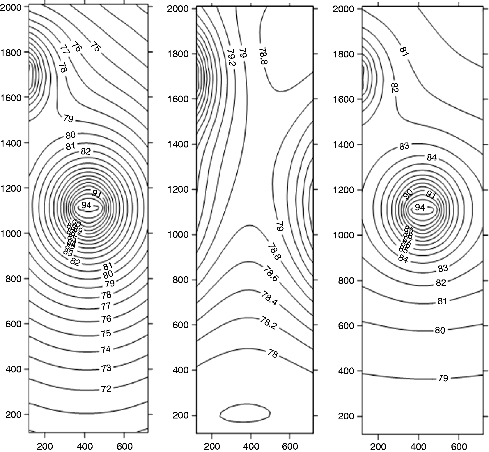

A validation process in noise modelling was conducted in order to determine a global estimation of deviation values. Three omnidirectional loud speakers (i.e. sound sources) were located in the room (same as the one in the numerical simulation, Figure 4); the sound emitted was white type and the mean power level emitted by three sources were adjusted to the level used in numerical example. A Type-I sound level meter with the facility of integration, and data logging in real time were used. The instrument was mounted on a tripod stand at a height of 100 cm above the ground. Then the measurement positions were selected on 90 cm × 60 cm grid patterns. A total of 242 measurements were taken at the above selected positions. The experimental results are presented together with the numerical simulations, to make it easy to compare them and to exploit the discrepancies (Figure 6). Comparison of experimental and calculated sound levels presented remarkably good agreement. However, a systematic difference can be seen between the measured and predicted values, and the mean square error is 1.2 dB. This result is quite obvious, as measured levels include the contribution from ceiling and multiple reflections and predicted values consider the simplified calculations of the propagation.

Figure 6.

Comparison of the experimental/calculated levels.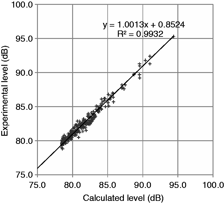

Discussion

A contour map showing noise distribution provides employers with useful information by clearly identifying areas where noise hazards exist by graphically representing sound pressure levels (i.e. noise levels). This makes it easier to calculate the noise exposure that employees undertaking tasks at particular locations are likely to be exposed to. The procedure presented in this study shows that noise contour maps can predict hazardous noise areas in industrial buildings. It is possible to obtain a noise contour map for any buildings and for any polygonal configuration. Changing the location of the machinery in the area affects the noise levels in the area. A noise map is studied when considering different workplace layouts and machine location simulations are created when new machines are placed in the building. To be most effective, noise control efforts should be based on the best available information, including predictions or measurements. Noise contour mapping can assist in deciding the most cost-effective allocation of resources for noise control. Noise contours also provide a basis for relocating noise sources, locating employee workstations, and determining hearing protection requirements.

With more than one surface, second-order image sources are generated, corresponding to rays that have experienced multiple reflections. Continuing in this manner, more image sources are generated, the propagation path increases, and the corresponding energy contribution decreases. The number of reflections increases until the rays arrive at a perfectly absorbent surface or their energy content becomes increasingly small. Increasing reflection order leads to an exponential increase in image sources and an exponential increase in computation time, making the method ineffective.

It is sometimes necessary to manage simultaneous noise contributions from multiple sources which require many repetitive calculations. The development of computer codes would be useful for this. Until these codes are developed, a spreadsheet program is useful. Spreadsheets display information in row and column format. Formulae are written according to cells identified by their row and column intersection, but may be replicated automatically for a range of cells.

The designer/engineers should have a basic understanding of how to justify the effects of acoustic characteristics of room on sound pressure level. A fundamental quality that determines the sound behavior of room is reverberance, primarily a function of the sound absorption in the room. The more area an absorbing material presents to incident sound, the more energy is absorbed. Most real rooms have a variety of surfaces with different materials. Absorption coefficients for commercially available materials are measured and published by manufacturers. Frequency-dependent absorption may be determined by experimental procedures, either using an impedance tube or using a reverberation chamber. The absorption coefficient α in equation (4) can be treated in terms of an average or frequency-dependent coefficient, but the computational process becomes more complicated while using frequency-dependent coefficient. The higher the absorption is, the lower the overall level which results. For larger absorptions, and a uniform distribution of absorption around the room, the Sabine or Eyring equation can be used to related absorption to reverberation time. Adding absorption is only justifiable if the reverberant field is dominant. Absorption on walls or ceilings will have little or no effect in the direct field, i.e. in the immediate vicinity of a noise source.

These effects due to the wave nature of sound depend directly on the wavelength of sound, i.e. diffraction and interference being more pronounced at low frequencies, while scattering due to the roughness of surfaces is more pronounced at high frequencies. A sound field in an enclosure is composed of many single waves. Each of them has its own particular amplitude, phase, and direction. However, when different conditions are fulfilled, it is possible to ignore these, and then it is in consideration of the existence in the enclosure of a diffuse sound field. The existence of diffuse sound field in an enclosure allows the application of simplified prediction models, and also of some important simplifications, e.g. negation of interference. It has been said that geometrical room acoustics can reflect only a partial aspect of the acoustical phenomena involved in a room, but that, however, is an aspect of great importance.²³

As stated by Kuttruff,²³ using wave theory to resolve sound propagation is extremely difficult. Instead, a simpler method of description – as with geometrical optics – uses the limiting case of increasingly small wavelengths, that is, the limiting case of high frequencies. Therefore, sound wave nature is neglected and sound propagation is studied using a method similar to sound ray propagation study. This assumption is valid when the sound wavelength is small relative to the room surface areas and large compared relative to their roughness. These conditions are frequently met in room acoustics. The image-source method reflects only some acoustic phenomena in a room, but that these phenomena are important. Nevertheless, it is a popular method for computer simulation of room acoustics and especially for simulation of early reflections because only low-order reflections are modeled. This makes the model impractical for modeling parts of the impulse response other than a few of the lowest order reflections.

Conclusion

A generalized image model is proposed to calculate the sound pressure level in an irregular-shaped room. This study presents an alternative technique to map noise levels in an industrial building. This analytical approach is practical and simple. The noise map generated shows noise distribution by graphically representing sound pressure levels, which is the level of noise in the building. The noise map can be a useful tool for studying and determining the effect of critical exposure areas. A noise map assists those responsible for safety and health protection at work to decide on what protective measures to implement. For instance, it may be desirable for noise management to evaluate noise distribution in a plant building before construction.

Footnotes

Funding

This research received no specific grant from any funding agency in the public, commercial, or not-for-profit sectors.

Conflict of interest

None declared.

References

Eleftheriou

. Industrial noise and its effects in human hearing. Appl Acoustics 2002; 63: 35–42.

Muzet

. Environmental noise, sleep and health. Sleep Med Rev 2007; 11: 135–142.

Thompson JK, Mitchell LD and Hurst CJ. A modified room acoustics approach to determine sound-pressure levels in irregularly- proportioned factory spaces. Inter-Noise 76: Proceedings of the international conference on noise control engineering, Washington, D.C., USA, 1976, pp. 465–468.

van Kempen EEMM, Staatsen BAM and van Kamp I. Selection and evaluation of exposure-effect relationships for health impact assessment in the field of noise and health. RIVM report no. 630400001, National Institute for Public Health and the Environment, Netherlands, http://rivm.openrepository.com/rivm/bitstream /10029 /7412/1/630400001.pdf (2005, accessed 29 March 2013).

Sbihi

Davies

Demers

. Hypertension in noise-exposed sawmill workers – a cohort study. Occup Environ Med 2008; 65: 643–646.

Tomei

Fioravanti

Cerratti

. Occupational exposure to noise and the cardiovascular system: A meta-analysis. Sci Total Environ 2010; 408: 681–689.

Edwards

Green

. Effect of an improved hearing conservation program on earplug performance in the workplace. Noise Control Eng J 1987; 28: 55–65.

European Directive 89/392/EEC Machinery Directive. Official Journal of the European Communities, 23 July 1998; L 207/20.

European Directive 2000/14/EC Noise Emission in the Environment by Equipment for Use Outdoors. Official Journal of the European Communities, 3 July 2000; L 162/1–L 162/78.

10.

European Directive 2006/42/EC New Machinery Directive. Official Journal of the European Union, 9 June 2006; L 157/49.

11.

Health and Safety Executive, UK. Controlling noise at work: the control of noise at work – guidance on regulations. ISBN 9780717661644, 2005; 1–130.

12.

Ondet

Barbry

. Modeling of sound propagation in fitted workshops using ray-tracing. J Acoust Soc Am 1989; 85: 787–796.

13.

Hodgson

. When is diffuse-field theory applicable? Appl Acoust 1996; 49: 197–207.

14.

Hodgson

. Sound-propagation curves in industrial workrooms: statistical trends and empirical prediction models. Build Acoust 1996; 3: 25–32.

15.

Cotana

. An improved room acoustics model. Appl Acoust 2000; 61: 1–25.

16.

Hodgson

. Experimental evaluation of simplified models for predicting noise levels in industrial workrooms. J Acoust Soc Am 1998; 103: 1933–1939.

17.

Kuttruff H. Sound propagation in working environments: Proceedings of 5th FASE symposium, Thessaloniki, 1985; 69–73.

18.

Ducourneaua

Planeaub

. The average absorption coefficient for enclosed spaces with non-uniformly distributed absorption. Appl Acoust 2003; 64: 845–862.

19.

Beranek

. Analysis of Sabine and Eyring equations and their application to concert hall audience and chair absorption. J Acoust Soc Am 2006; 120: 1399–1410.

20.

Nanthavanij

Boonyawat

Wongwanthanee

. Analytical procedure for constructing noise contours. Int J Indus Ergon 1999; 23: 123–127.

21.

Allen

Berkley

. Image method for efficiently simulating small-room acoustics. J Acoust Soc Am 1979; 65: 943–950.

22.

Gibbs

Jones

. A simple image method for calculating the distribution of sound pressure levels within an enclosure. Acustica 1972; 26: 24–32.

23.

Kuttruff

. Room acoustics, Barking: Elsevier Science, 1991.