Short-term load forecasting coupled with weather profile generation methodology

Abstract

Short-term building load forecasting is indispensable in daily operation of future intelligent/green buildings, particularly in formulating system control strategies and assessing the associated environmental impacts. Most previous research works have been focused on studying the advancement in forecasting techniques, but not as much on evaluating the availability of influential factors like the predicted weather profile in the coming hours. This article proposes an improved procedure to predict the building load 24 hours ahead, together with a backup weather profile generating method. The quality of the proposed weather profile generation model and the forecasting procedures were examined through a case study of application to university academic buildings. The results showed that the load forecasting accuracy with the application of either the real weather data on record or of the predicted weather data from the profile generation model is very much similar. This indicates that the weather prediction model is suitable for applying to building load forecasting. Besides, the comparisons between different sets of input data illustrated that the forecasting accuracy can be improved through the input data filtering and regrouping procedures.

Practical application : A weather profile prediction technique for use in building energy forecasting was introduced. This can be coupled to a building energy use forecasting model for predicting the hourly consumption profile of the next day. This prediction time span can be crucial for formulating the daily operation plan of the utility systems or for smart micro-grid applications. The appropriateness of the methodology was evaluated through a case study.

Keywords

Building energy consumption weather forecasting data filtering and regrouping short-term load forecasting

Introduction

Building load forecasting methods are generally categorized by the prediction time span as follows^1,2: (a) long-term forecast of more than one year ahead, (b) medium-term forecast from one week ahead to one-year ahead, and (c) short-term forecast from fraction of an hour up to one week ahead. Short-term load forecasting (STLF) at the time span of 24 hours (one day) ahead is the focus of this study. This prediction time span of hourly profile can be crucial for formulating the daily operation plan of the utility systems or for smart micro-grid applications.³ A suitable STLF will enable the utility provider to observe and take control of the balance between the supply and demand sides. Accurate STLF of a micro-grid can enhance full system integration with renewable energy resources and to improve building system efficiency and save operating costs in response to the variation of electricity price.^4–7 Hence, STLF for a day ahead can be a very useful means in energy management.

In real buildings, the electricity load curves carry much variability, noise and non-linear characteristics. The occupant activities and operating schedules vary considerably with the building type, location, and perhaps more important for air-conditioned buildings, the weather conditions.⁸ Numerous external and internal factors co-exist⁹ and this led to the formulation of different STLF models.^10–14 In order to show the sophistication in modelling techniques, many of them choose to verify the prediction accuracy by comparing the calculation results based on historical weather data (like from local observatory records) with the past building load profile (like from energy management system record). But in reality, the actual weather data of tomorrow will never be available today for future building load projection. This dilemma calls for a return to the originality^15–17 of using either weather forecast data (that may be available from a third party institution) or a weather forecasting model for self-generation of the unknown data set.¹⁸ It comes to us that the former may not be always available or the acquisition may have substantial cost implication. For this reason, we have successfully developed a STLF model that goes together with an hourly weather forecasting technique. The following presents our works in detail, which include the technological review, the influential factors analysis, the proposed forecasting framework and finally a real case demonstration.

Technological background

Influential factors and data input

The energy use profile of a building can be taken as a multi-input mathematical function. The variation depends on four main interacting factors namely building structure, operation schedule, occupancy and weather conditions. In principle, the building structure is fixed once the building project is completed. The operating schedule and occupancy (including the usage characteristics, occupancy density and activities) can be taken as the internal factors,^19–28 of which the time elements are mostly included to mimic dynamic human behaviours. Many previous studies demonstrated that the historical performance at specific hours of the day and the day type could have great implication on the current hour of building energy consumption. In a university building, for example, academic calendar affects much the energy consumption pattern.

As far as STLF is concerned, the importance of individual influential factor is not the same in all building cases. The input data should be best filtered before loading for forecasting model development, and the filtering method can be either linear or nonlinear.^29–32 The linear analysis methods like regression and sensitive studies may not fit the nonlinearity between the influential factors and building energy consumption rate well. In order to deal with this, Kusiak et al.³³ proposed the boosting tree algorithm as a means of input data analysis, whereas Keynia³⁴ recommended the data mining method based on mutual information (MI) evaluation. These nonlinear feature selection methods are effective to filter out the irrelevant (or redundant) candidate inputs.

Forecasting models

Energy prediction techniques can be grouped into three categories: the classical engineering approach (white box), the data-driven statistical approach (black box) such as artificial neuron network (ANN) and the hybrid approach (grey box). An up-to-date classification is illustrated in Figure 1.³⁵ With the rapid development of modern meters, the data-driven forecasting method is now widely applied, like the ANN model as an example. ANN has been successfully applied for the prediction of the overall building energy consumption and also the cooling/heating demand without prior knowledge of the building geometry or the material thermal properties.^36–43

Figure 1.

The categories of building forecasting models.

New weather forecasting technique

A new weather forecasting model to generate the upcoming 24-hour weather profile is introduced below. This simple model uses the basic weather forecast information of the next day as input, such as the daily ranges of dry-bulb temperature and relative humidity. These figures are readily accessible via public media, like television or radio broadcast or public websites. As general reference, Figure 2 shows the typical daily variation of air temperature, relative humidity and global solar radiation of Hong Kong as a subtropical coastal city. Such hourly changes of weather conditions of some well-known cities can be available on international weather forecast channels. But in other places where the future hourly profiles remain absent, our proposed forecasting model can be applied.

Figure 2.

Typical daily weather profiles: (a) air temperature and relative humidity and (b) global solar radiation.

Temperature profile

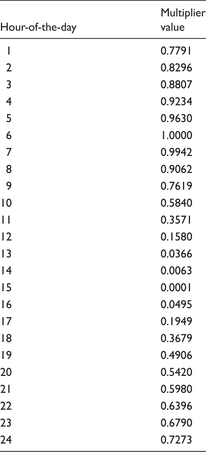
A typical 24-hour temperature profile has a ‘peak’ (T_max) and a ‘trough’ (T_min) across the day. The dry-bulb temperature T of each hour can be estimated by means of the normalized temperature range (known as the multiplier value β) as follows

T = T_{max} - β \cdot (T_{max} - T_{min})

(1)

β can be generated statistically from the past year temperature data. Figure 3(a) shows the yearly averaged 24-hour temperature profiles of Hong Kong in recent years (2012–2015). It can be seen that their cyclic patterns are more or less the same. The positions of the curves indicate that 2015 was much warmer than the previous three years. Figure 3(b) shows the four multiplier value β curves derived accordingly. From these, the 24-hour reference values of β for Hong Kong were determined and listed in Table 1.

Figure 3.

Derived yearly averaged 24-hour temperature profiles of Hong Kong for 2012–2015: (a) from actual observatory record and (b) normalized multiplier curves.

Table 1.

Reference multiplier values β for application in Hong Kong.

Hour-of-the-day	Multiplier value
1	0.7791
2	0.8296
3	0.8807
4	0.9234
5	0.9630
6	1.0000
7	0.9942
8	0.9062
9	0.7619
10	0.5840
11	0.3571
12	0.1580
13	0.0366
14	0.0063
15	0.0001
16	0.0495
17	0.1949
18	0.3679
19	0.4906
20	0.5420
21	0.5980
22	0.6396
23	0.6790
24	0.7273

Relative humidity

Based on the predicted ambient temperature of each hour and its definite relationship with the water vapour saturation pressure, the corresponding relative humidity can be determined from their high value (ϕ_max) and low value (ϕ_min) forecasting through the following steps, taking the fact that the water vapour pressure changes very little within a day.

Step 1: Calculate the water vapour saturation pressure from each dry-bulb temperature by

P_{qb} = 610 \cdot 10^{\frac{7.45 T}{235 + T}}

(2)

Step 2: Generate the reference water vapour pressure P_c by

P_{max} = ϕ_{max} \cdot p_{qb, max}

(3)

P_{min} = ϕ_{min} \cdot p_{qb, min}

(4)

P_{c} = 0.5 (P_{max} + P_{min})

(5)

where P_qb,max and P_qb,min are the daily maximum and minimum water vapour saturation pressure selected from the Step 1 data. Here, P_max and P_min frame the upper and lower bound water vapour pressure of the day.

Step 3: Calculate the relative humidity as

ϕ = \frac{P_{c}}{P_{qb}} \cdot 100 %

(6)

Global solar radiation

The generation of the 24-hour global solar radiation is based on the simple sky model^44,45 commonly used in solar energy simulation. On any calendar day (of day number d from 1 to 365), the time of sunrise and sunset at any position on Earth are fixed. By defining the daily angle θ as

θ = \frac{2 π}{365} (d - 1)

(7)

then the equation of time (Et) can be calculated as a function of θ, i.e.

\begin{matrix} Et = 229.18 \cdot [\begin{matrix} {\begin{matrix} 0.000075 + 0.001868 cos (θ) \\ + 0.032077 sin (θ) - 0.014615 cos (2 θ) \end{matrix}} \\ - 0.04089 sin (2 θ) \end{matrix}] \end{matrix}

(8)

where the factor 229.18 is for unit conversion from radians to minutes. Et denotes the difference between the true solar time and the mean solar time.

Solar declination δ is the angle in radians between the equatorial plane and the line connecting the centres of the Sun and the Earth. This can be calculated as

δ = 23.45 \cdot cos (2 π \frac{d - 173}{365}) \cdot \frac{π}{180}

(9)

where the value of 173 corresponds to the Julian day number of June 22 (Summer Solstice).

The solar angular hour is calculated as

\begin{matrix} h = co s^{- 1} (\frac{sin (\frac{- 0.833 π}{180}) sin (δ)}{cos (γ) cos (δ)}) \end{matrix}

(10)

where γ is the observer's latitude.

The number of hours of daylight (h_d) is determined as a function of h, in that

h_{d} = \frac{h}{7.5} \frac{180}{π}

(11)

Then the time of sunrise (t_sr) and sunset (t_ss) can be calculated as

t_{sr} = 12 - \frac{h_{d}}{2} - \frac{E_{t}}{60}

(12)

t_{ss} = 12 + \frac{h_{d}}{2} - \frac{E_{t}}{60}

(13)

In the simple sky model, the solar irradiance (I) is characterized by the time of sunrise and sunset, as well as the peak solar irradiance (I_max). At any time t of the day, this is given by

I = {\begin{matrix} 0, for t < t_{sr} or t > t_{ss} \\ I_{max} sin (\frac{π (t - t_{sr})}{t_{ss} - t_{sr}}), t_{sr} \leq t \leq t_{ss} \end{matrix}

(14)

where I_max is related to the daily maximum extraterrestrial irradiance (I_ETI,max) through the ratio coefficient (kt), i.e.

I_{max} = I_{ETI, max} \cdot kt

(15)

By definition, I_ETI is a function of the solar constant I₀ (at 1362 W/m²), the eccentricity correction factor E₀ and the zenith angle ψ, i.e.

I_{ETI} = I_{0} E_{0} cos ψ = 1362 (1 + 0.033 cos (\frac{2 π d}{365})) cos ψ

(16)

The value of ψ depends on the local time. On the other hand, kt in each month can be found from a simple regression model as a function of temperature and humidity, i.e.

kt = f (T, ϕ) = x_{0} + x_{1} T + x_{2} ϕ + x_{3} T^{2} + x_{4} ϕ^{2}

(17)

where x₀ to x₄ are the reference coefficients. For example, with the use of the past year data (2013–2014), the values of x₀ to x₄ in each of the 12 months for the case of Hong Kong are derived as listed in Table 2.

Table 2.

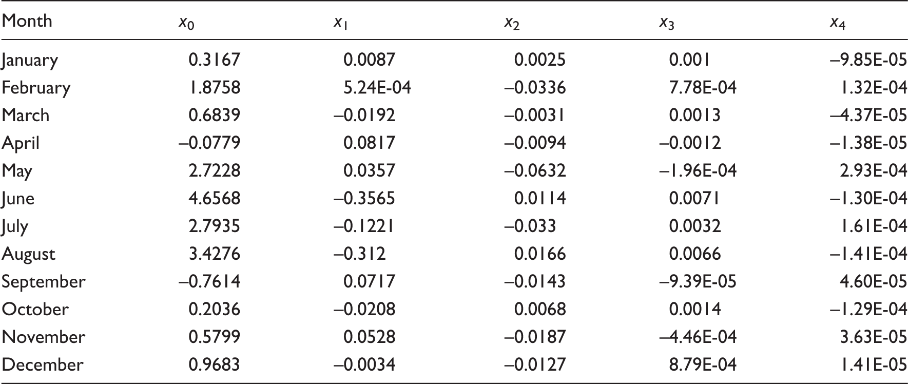
Derived reference coefficients of k_t regression equation of Hong Kong.

Month	x ₀	x ₁	x ₂	x ₃	x ₄
January	0.3167	0.0087	0.0025	0.001	–9.85E-05
February	1.8758	5.24E-04	–0.0336	7.78E-04	1.32E-04
March	0.6839	–0.0192	–0.0031	0.0013	–4.37E-05
April	–0.0779	0.0817	–0.0094	–0.0012	–1.38E-05
May	2.7228	0.0357	–0.0632	–1.96E-04	2.93E-04
June	4.6568	–0.3565	0.0114	0.0071	–1.30E-04
July	2.7935	–0.1221	–0.033	0.0032	1.61E-04
August	3.4276	–0.312	0.0166	0.0066	–1.41E-04
September	–0.7614	0.0717	–0.0143	–9.39E-05	4.60E-05
October	0.2036	–0.0208	0.0068	0.0014	–1.29E-04
November	0.5799	0.0528	–0.0187	–4.46E-04	3.63E-05
December	0.9683	–0.0034	–0.0127	8.79E-04	1.41E-05

Results verification

In order to verify the accuracy of the above weather prediction model, we compared the generated results of air temperature, relative humidity and global solar radiation from this proposed model with the Hong Kong Observatory record. This was for the whole year 2015 and with the year round weather forecast data coming from an international website.⁴⁶ Table 3 gives the mean absolute percentage error (MAPE) value of each month and of the whole year as well. Reasonably good accuracy can be observed, particularly for the summer months when the building energy consumption was high. The year round MAPE is around 3.2% for air temperature, 5.7% for relative humidity and 11.3% for solar radiation. It should be noted that weather forecast made by any authority like a local observatory station may not be accurate in the first place. Figures 4(a) to (c) show the graphical comparisons of model predicted and actual air temperature, relative humidity and global solar radiation, respectively, taking the first week of August 2015 for reference.

Table 3.

Mean absolutely precentage error of the predicted weather data against the official record of year 2015.

	Dry-bulb temperature	Relative humidity	Global solar radiation
January	4.2411%	8.4702%	22.9650%
February	3.7502%	6.0143%	12.3440%
March	3.4454%	4.9317%	14.5652%
April	3.6252%	5.6472%	4.2227%
May	3.5696%	5.3679%	5.4517%
June	2.4390%	4.8914%	7.6463%
July	2.8610%	5.5037%	2.3042%
August	2.5094%	5.2188%	3.1516%
September	2.5355%	4.7487%	5.1917%
October	2.9878%	6.2498%	16.1013%
November	2.7412%	4.9994%	16.6804%
December	3.9891%	6.3309%	25.0522%
Overall	3.2245%	5.6978%	11.3064%

Figure 4.

Weather prediction model verification: (a) temperature, (b) relative humidity and (c) global solar radiation.

New STLF model

The general framework of our STLF model is given in Figure 5, which illustrates the flow processes of data preparation, filtering, regrouping and then the forecast model structure optimization. At first, based on the full list of anticipated influential factors, the raw input data set is sorted for analysis. Then, the importance of these influential factors is ranked. The less important factors will be filtered out, subject to the screening criteria. Afterwards, the input data on calendar-day 24-hour basis are regrouped into sub-sets based on the distinct energy consumption characteristics. For illustration convenience, the decision of forming two data sub-sets as the result is assumed in Figure 5. Then for each data set, the forecasting model structure is optimized through error analysis. The above-described stages are further elaborated below:

(a) Data filtering: Filtering the input data is needed in order to overcome the curse of dimensions which caused by irrelevant and redundant candidate inputs. So before the confirmation of input variables, the input data are to be analysed using the MI criterion. The involved influential factors will have the individual MI values calculated then their importance ranked. The detailed algorithm can be found in Keynia.³⁴ The overview of this data filtering process can be seen in Figure 6.

(b) Data regroup: Building energy consumption usually has its case-specific trend characteristic. It will have similar daily consumption profile during the same operation schedule, independent of the weather condition. Based on the building operation schedule and the energy consumption outcome, the input data can be regrouped into sub-sets consisted of 24-hour daily data as the group members. Then, a distinct forecasting model will be worked out for each sub-set. This modelling procedure will lead to more accurate predictions. The details of this part of data handling can be referred to our case study in section ‘Case study’.

(c) Forecasting model and structure optimization: Our forecasting model is based on ANN model with back-propagation and Levenberg-Marquardt learning method. Figure 7 shows an example of the ANN architecture. In order to achieve high computation speed, only one hidden layer was adopted. As the results accuracy can be sensitive to the transfer function and the neuron numbers of the hidden layer,³¹ systemic comparison runs should be performed in the model structure optimization process, which can be seen in the section ‘Energy consumption analysis and data regrouping’.

(d) Accuracy evaluation criteria: The following three accuracy criteria are commonly used to assess forecasting model effectiveness: the MAPE, the Daily Peak MAPE, and the coefficient of variance of the root mean squared error (CVRMSE) under 95% confidence limits.⁴⁷ By definition

MAPE = \frac{1}{N} \sum_{i = 1}^{N} \frac{| Y_{a, i} - Y_{p, i} |}{Y_{p, i}} \cdot 100 %

(18)

DailyPeakMAPE = \frac{| max Y_{a} - max Y_{p} |}{max Y_{a}} \cdot 100 %

(19)

CVRMSE = \frac{\sqrt{\frac{\sum_{i = 1}^{N} {(Y_{a, i} - Y_{p, i})}^{2}}{\bar{Y}}}}{max Y_{a}} \cdot 100 %

(20)

where N is the sample size, Y_a is the actual load, Y_p is the predicted load and

\bar{Y}

is the mean of the actual loads. While the Daily Peak MAPE indicates the behaviour of the daily load peaks forecasting, the CVRMSE indicates the uncertainty in the forecast procedure.

Figure 5.

Forecasting flowing chart.

Figure 6.

Overview of data filtering process.

Figure 7.

ANN forecasting model architecture. ANN: artificial neuron network.

Case study

A case study is introduced in this section as an illustrating example. This case study involved two multi-story academic buildings in our university campus. Building No. 1 was an older building built over 20 years ago. Building No. 2 was relatively new, of age less than five years. Energy is supplied from the mains electrical grid. The two buildings were fully air conditioned with year-round space cooling demand. Their daily operation schedules were the same, with opening hours from 7:00 to 23:00 on normal weekdays and 7:00 to 18:00 during weekends. The university operation was according to the academic calendar with four distinct period types: teaching semester, student revision week, examination period and semester break.

Data preparation and filtering

From the past years record, the available forecast/actual weather data, historical energy consumption record and academic calendar period type of each day were gathered for formulating the forecast model. They were used as the input data to predict the 24-hour energy consumption profile of the following day. Weather data of 2013 and 2014 were first collected from the Hong Kong Observatory. These include dry-bulb temperature, relative humidity, global solar radiation, rainfall, clearness of sky, cloud condition and wind speed. The energy consumption data were the hourly electricity consumption record of each building extracted from the central energy management system. Influential factors were identified based on the findings of the previous works and also the available data at hand.

A total of nine influential factors were taken part in the filtering process. They were the dry-bulb temperature, relative humidity, global solar radiation, sky clearness, cloud condition, wind speed, rainfall, hour number of the day and the corresponding energy consumption of the same hour one day before. Their importance ranking based on MI values is shown in Table 4. The threshold was arbitrary chosen as 0.4 and based on this, six influential factors were selected as the initial input variables in deriving the ANN model. Nevertheless, in practice, wind speed data are generally not provided on weather forecasting websites and are not well correlated to the other weather parameters/information for facilitating its forecast model development. For these reasons, we utilized the recorded weather data to quantify its influence on the prediction of energy consumption in both Buildings No. 1 and No. 2 through error analysis. The results are shown in Table 5. It can be seen that for the prediction cases with or without the inclusion of wind speed in the ANN model, there are small differences in MAPE percentage (generally less than 0.2%). Therefore, our final ANN model as in Figure 7 includes only five input variables.

Table 4.

Energy consumption influential factor analysis.

Influential factors	MI value	Rank
Dry-bulb temperature	0.9547	2
Humidity	0.9494	3
Global solar radiation	0.7011	4
Clearness of the sky	0.2547	7
Cloud condition	0.1670	8
Wind speed	0.5844	5
Rainfall	0.1149	9
Hour-of-the-day	0.4030	6
Previous day energy consumption data	0.9817	1

MI: mutual information.

Table 5.

Comparison of mean absolutely percentage error in energy prediction – with or without wind speed.

Building	Record weather data without wind speed			Record weather data with wind speed
Building	Set 1	Set 2	Overall	Set 1	Set 2	Overall
No. 1	4.9695%	7.0423%	5.9775%	4.8204%	6.8310%	5.7802%
No. 2	8.7464%	10.6906%	9.3995%	8.6589%	10.5837%	9.3055%

Energy consumption analysis and data regrouping

Before performing the forecast model evaluation, the energy consumption behaviour of these two buildings in 2013 and 2014 was analysed. Figures 8(a) to (f), respectively, show the load cloud charts of Buildings No. 1 and No. 2 and for three calendar months with seasonal representation, i.e. August 2013 for summer, April 2014 for spring and December 2014 for winter. In these charts, the x-axis shows the calendar dates and the y-axis shows the daily hours 1–24.

Figure 8.

Energy consumption (kW) cloud charts of Buildings No. 1 and No. 2. (a) Building No. 1 in August 2013, (b) Building No. 2 in August 2013, (c) Building No. 1 in April 2014, (d) Building No. 2 in April 2014, (e) Building No. 1 in December 2014 and (f) Building No. 2 in December 2014.

The daily profile and weekly trend can be readily observed from the colour distribution patterns, in that, the situations of both buildings look alike. In general, at night from 00:00 AM to 8:00 AM, the energy consumption level was very low. Then after 8:00 AM, the energy consumption increases rapidly, reaching the peak level in between 14:00 PM and 17:00 PM. Then after 20:00 PM, the energy consumption decreases.

In all six monthly charts, the daily energy consumption as shown follows weekly cyclic characteristics. From Monday to Friday, the daily consumption was fairly stable. Comparatively, the weekend consumption was low. But exceptional cases of low consumption during holidays can be found – like the Easter holiday in April and the Christmas period in December. These were the student holidays. Also, August 14 was the day under typhoon attack, on which students were evacuated. So generally speaking, the normal weekday's energy consumption profile (Data Set 1) is distinctively different from the other days' profile of low consumption level (Data Set 2). Hence, the input data were regrouped accordingly. In the model structure optimization process, the 2013–2014 weather forecast data were made use of. The results showed that for Set 1 and Set 2, respectively, the best transfer function combinations are logsig/purelin and tansig/purelin, and the optimal neuron numbers are 3 and 16, seen in Tables 6 and 7.

Table 6.

Testing mean absolutely percentage error of different transfer function combinations.

	TF groups		Set 1	Set 2
1	purelin	purelin	6.5975%	11.4372%
2	logsig	purelin	6.111%	8.1324%
3	tansig	purelin	6.4061%	7.597%
4	purelin	logsig	25.0941%	20.5301%
5	logsig	logsig	29.1844%	23.6876%
6	tansig	logsig	29.4187%	24.33%
7	purelin	tansig	9.2747%	12.4776%
8	logsig	tansig	12.7211%	12.8559%
9	tansig	tansig	13.9047%	14.6423%

Table 7.

Testing mean absolutely percentage error of different neurons number.

Neuron numbers	Set 1	Set 2
2	5.7156%	8.0723%
3	5.5772%	7.9376%
4	5.9400%	7.7928%
10	5.9345%	7.4027%
15	5.6383%	7.3503%
16	5.6426%	7.3483%
17	5.6508%	7.3503%
28	5.7918%	7.4237%
30	5.8209%	7.4443%

Forecasting results and error analysis

The rationale of our proposed methodology was tested by comparing the predicted energy consumption with the actual records of 2015, and also the error analysis. The results of comparison and analysis can be found in Figure 9 and Figure 10, Tables 8 and 9. Our comparisons show that the results of forecasting agree well with the real load consumption, as reflected in Figures 9(a) and (b) for Buildings No. 1 and No. 2, respectively. For each building, two sets of prediction results were acquired with the use of the same energy forecasting model. The difference was in their weather data input, in that, data from the weather forecast model were applied in the first trial, but actual hourly weather data of the day were used in the second trial and then compared. It was found that the prediction accuracy was very good for both trials. Figure 9 shows the graphical plots for a summer week. Both load prediction curves show comparable performance with the actual consumption. The forecasting error distribution has good agreement with normal distribution, seen in Figure 10, which shows the reasonable of prediction results.

Figure 9.

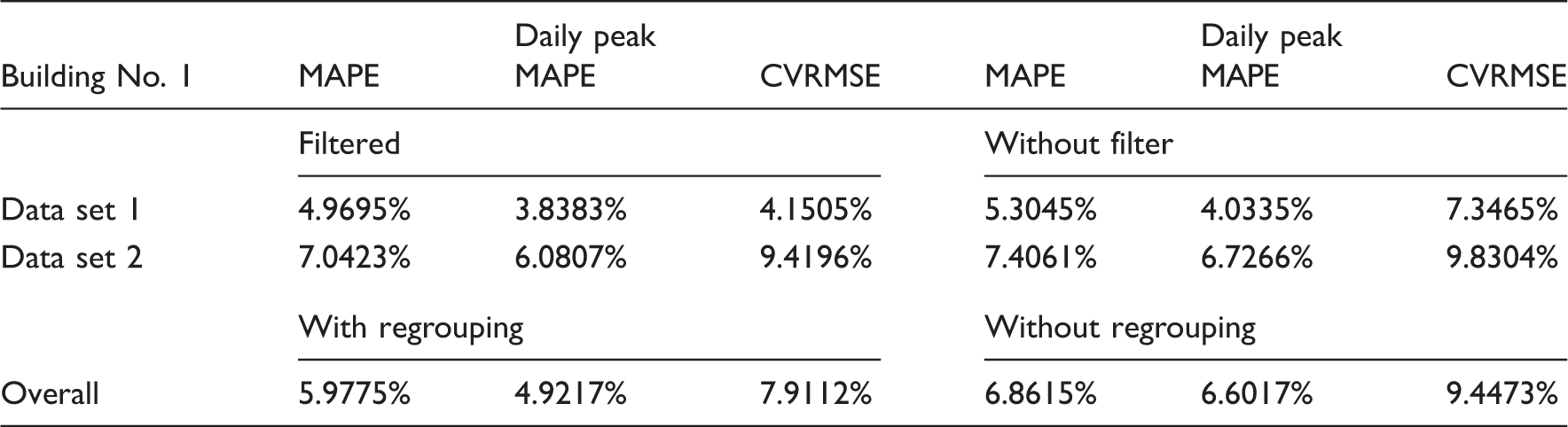
Results comparison of load forecasting for the week 8–14 July 2015 using different weather data sets: (a) Building No. 1 and (b) Building No. 2.

Figure 10.

Forecasting error distribution analysis. (a) Building 1: Prediction with record weather data, (b) Building 1: Prediction with forecast weather data, (3) Building 2: Prediction with record weather data and (d) Building 2: Prediction with forecast weather data.

Table 8.

Comparison of mean absolutely percentage error in energy prediction – actual weather data against forecast.

Building	Record weather data			Forecasting weather data
Building	Set 1	Set 2	Overall	Set 1	Set 2	Overall
No. 1	4.9695%	7.0423%	5.9775%	5.1195%	6.9788%	6.0245%
No. 2	8.7464%	10.6906%	9.3995%	8.6177%	10.5956%	9.1893%

Table 9.

Forecasting errors with or without input data filtering and regrouping.

Building No. 1	MAPE	Daily peak MAPE	CVRMSE	MAPE	Daily peak MAPE	CVRMSE
	Filtered			Without filter
Data set 1	4.9695%	3.8383%	4.1505%	5.3045%	4.0335%	7.3465%
Data set 2	7.0423%	6.0807%	9.4196%	7.4061%	6.7266%	9.8304%
	With regrouping			Without regrouping
Overall	5.9775%	4.9217%	7.9112%	6.8615%	6.6017%	9.4473%

CVRMSE: coefficient of variance of the root mean squared error; MAPE: mean absolute percentage error.

Also from Table 8, it can be concluded that the MAPE differences (of only less than 0.2%) of the predicted energy consumption based on the weather data obtained from the forecast model and from the real weather data are very small. This so happens to both buildings. The quality of the weather profile prediction technique is therefore fully demonstrated. Generally speaking, the modelling accuracy of Building No. 1 is better than Building No. 2. This is because the occupancy in the older building is more stable than in the new Building No. 2.

The effectiveness of having filtering and regrouping in this case study was evaluated making use of the Building No.1 performance. The results of forecasting errors are shown in Table 9. It can be seen that for both Set 1 and Set 2, the prediction accuracy can be improved with filtering. The use of more influential factors (without filter) was not helpful at all. So, the filtering process is proved appropriate. The same conclusion can be reached with the use of regrouping, as demonstrated by the error analysis with the use of the same evaluation parameters. It is worth mentioning that the MAPE of 5.98% in this case study with filtering is generally lower than those quoted in the previous related studies, like those in Bagnasco et al.,³¹ Dong et al.,⁴¹ Yuce et al.⁴² and Marmaras et al.⁴³ are 7.0%, 9.26%, 6.51% and 6.7%, respectively.

Conclusion

This paper proposed a framework to predict the short-term building load with data filtering and regrouping which will improve the forecasting accuracy. It also provides a backup weather forecasting method to generate the needed weather data used in the load forecasting model. The main conclusion of this paper is listed below:

(1) The input data filtering procedures show that dry-bulb temperature, relative humidity and global solar radiation were important influencing factors, so was the energy consumption level of the same hour one day before.

(2) Observations through the cloud charts identified the necessity of data regrouping based on normal weekday and the remaining periods of the academic calendar. The subsequent error analysis confirms the effectiveness of input data filtering and regrouping to improve the forecasting model accuracy.

(3) The proposed weather forecasting method could be used as backup approach to generate the needed data for the load prediction model, especially for the case without large variation of occupancy and climate. In order to extend the adaptivity of the proposed model, more case study need to be consider in our future work.

Footnotes

Declaration of conflicting interests

The author(s) declared no potential conflicts of interest with respect to the research, authorship, and/or publication of this article.

Funding

The author(s) disclosed receipt of the following financial support for the research, authorship, and/or publication of this article: The work described in this article was financially supported by the Contract Research Grants of the City University of Hong Kong (Project no. 9231136).

Appendix

References

Gonzalez-Romera

Jaramillo-Moran

Carmona-Fernandez

. Monthly electric energy demand forecasting based on trend extraction. IEEE Trans Power Syst 2006; 21: 1946–1953.

Kyriakides

Polycarpou

. Short term electric load forecasting: a tutorial, trends in neural computation. Stud Comput Intell 2007; 35: 391–418.

Borges

Penya

Fernández

et al.

Assessing tolerance-based robust short-term load forecasting in buildings. Energies 2013; 6: 2110–2129.

Massana

Pous

Burgas

et al.

Short-term load forecasting in a non-residential building contrasting models and attributes. Energ Build 2015; 92: 322–330.

Bruni

Cordiner

Mulone

et al.

A study on the energy management in domestic micro-grids based on Model Predictive Control strategies. Energ Convers Manag 2015; 102: 50–58.

Chung

Park

Coimbra

CFM

. Estimation of the building energy loads and LNG demand for a cogeneration-based community energy system: a case study in Korea. Energ Convers Manag 2014; 87: 1010–1026.

Mayer

Killian

Kozek

. Management of hybrid energy supply systems in buildings using mixed-integer model predictive control. Energ Convers Manag 2015; 98: 470–483.

Penya

Borges

Agote

et al.

Short-term load forecasting in air-conditioned non-residential Buildings. IEEE Int Symp Ind Electron 2011; 978: 1359–1364.

Leung

Tse

Lai

et al.

The use of occupancy space electrical power demand in building cooling load prediction. Energ Build 2012; 55: 151–163.

10.

Chitsaz

Shaker

Zareipour

et al.

Short-term electricity load forecasting of buildings in micro grids. Energ Build 2015; 99: 50–60.

11.

Grant

Eltoukhy

Asfour

. Short-term electrical peak demand forecasting in a large government building using artificial neural networks. Energies 2014; 7: 1935–1953.

12.

Iwafune Y, Yagita Y, Ikegami T, et al. Short-term forecasting of residential building load for distributed energy management. In: IEEE International Energy Conference, Cavtat, Croatia, 13–16 May 2014, pp.1197–1204.

13.

Chae

Horesh

Hwang

et al.

Artificial neural network model for forecasting sub-hourly electricity usage in commercial buildings. Energ Build 2016; 111: 184–194.

14.

Bacher

Madsen

Nielsen

et al.

Short-term heat load forecasting for single family houses. Energ Build 2013; 65: 101–112.

15.

Friedrich

Afshari

. Short-term forecasting of the Abu Dhabi electricity load using multiple weather variables. Clean Efficient Affordable Energ Sustain Future 2015; 75: 3014–3026.

16.

Roldán-Blay

Escrivá-Escrivá

Álvarez-Bel

et al.

Upgrade of an artificial neural network prediction method for electrical consumption forecasting using an hourly temperature curve model. Energ Build 2013; 60: 38–46.

17.

Lazos

Sproul

Kay

. Development of hybrid numerical and statistical short term horizon weather prediction models for building energy management optimization. Build Environ 2015; 90: 82–95.

18.

Wang

Cheng

. A research on a following day load simulation method based on weather forecast parameters. Energ Convers Manag 2015; 103: 691–704.

19.

Haldi

Robinson

. The impact of occupants' behaviour on building energy demand. J Build Perform Simulat 2011; 4: 323–338.

20.

Parys

Saelens

Hens

. Coupling of dynamic building simulation with stochastic modelling of occupant behaviour in offices – a review based integrated methodology. J Build Perform Simulat 2011; 4: 339–358.

21.

Dipti

Chang

Liew

. Demand forecasting using fuzzy neural computation with special emphasis on weekend and public holiday forecasting. Power Syst IEEE Trans 1995; 10: 1897–1903.

22.

Page

Robinson

Morel

et al.

A generalised stochastic model for the simulation of occupant presence. Energ Build 2008; 40: 83–98.

23.

Zhang

Patuwo

. Forecasting with artificial neural networks: the state of the art. Int J Forecast 1998; 14: 35–62.

24.

Dillon

Sestito

Leung

. Short term load forecasting using an adaptive neural network. Int J Electr Power Energ Syst 1991; 13: 186–192.

25.

Papalexopoulos AD, Shangyou H and Tie-Mao P. Application of neural network technology to short-term system load forecasting. In: Athens Power Tech, 1993. APT 93. Proceedings. Joint International Power Conference, Athens, 5–8 September 1993, pp. 796–800. Piscataway, NJ: IEEE.

26.

Kreider

Curtiss

Rabl

. Heating and cooling of buildings: design for efficiency, 2nd ed. New York, NY: CRC Press, 2011.

27.

Aydinalp

IsmetUgursal

Fung

. Modeling of the appliance, lighting, and space-cooling energy consumptions in the residential sector using neural networks. Appl Energ 2002; 71: 87–110.

28.

Kwok

SSK

Lee

EWM

. A study of the importance of occupancy to building cooling load in prediction by intelligent approach. Energ Convers Manag 2011; 52: 2555–2564.

29.

Dong

Lee

Sapar

. A holistic utility bill analysis method for baselining whole commercial building energy consumption in Singapore. Energ Build 2005; 37: 167–174.

30.

Amber

Aslam

Hussain

. Electricity consumption forecasting models for administration buildings of the UK higher education sector. Energ Build 2015; 90: 127–136.

31.

Bagnasco

Fresi

Saviozzi

et al.

Electrical consumption forecasting in hospital facilities: an application case. Energ Build 2015; 103: 261–270.

32.

Lü

Kibert

et al.

Modeling and forecasting energy consumption for heterogeneous buildings using a physical-statistical approach. Appl Energ 2015; 144: 261–275.

33.

Kusiak

Zhang

. A data-driven approach for steam load prediction in buildings. Appl Energ 2010; 87: 925–933.

34.

Keynia

. A new feature selection algorithm and composite neural network for electricity price forecasting. Eng Appl Artif Intell 2012; 25: 1687–1697.

35.

Fumo

. A review on the basics of building energy estimation. Renew Sustain Energ Rev 2014; 31: 53–60.

36.

Foucquier

Robert

Suard

et al.

State of the art in building modelling and energy performances prediction: a review. Renew Sustain Energ Rev 2013; 23: 272–288.

37.

Ahmad

Hassan

Abdullah

et al.

A review on applications of ANN and SVM for building electrical energy consumption forecasting. Renew Sustain Energ Rev 2014; 33: 102–109.

38.

Guo

Nazarian

et al.

Hourly cooling load forecasting using time-indexed ARX models with two-stage weighted least squares regression. Energ Convers Manag 2014; 80: 46–53.

39.

Kalogirou

. Applications of artificial neural networks in energy systems – a review. Energ Convers Manag 1999; 40: 1073–1087.

40.

Kwok

SSK

Lee

EWM

. A study of the importance of occupancy to building cooling load in prediction by intelligent approach. Energ Convers Manag 2011; 52: 2555–2564.

41.

Dong

Rahman

SMM

et al.

A hybrid model approach for forecasting future residential electricity consumption. Energ Build 2016; 117: 341–351.

42.

Yuce

Mourshed

Rezgui

. A smart forecasting approach to district energy management. Energies 2017; 10: 1073.

43.

Marmaras

Javed

Cipcigan

et al.

Predicting the energy demand of buildings during triad peaks in GB. Energ Build 2017; 141: 262–273.

44.

Iqbal

. An introduction to solar radiation, New York, NY: Elsevier, 1983.

45.

Reda

Andreas

. Solar position algorithm for solar radiation applications. Sol Energ 2004; 76: 577–589.

46.

AccuWeather. Weather data source, https://www.accuweather.com/en/hk/hong-kong-weather (accessed 15 May 2016).

47.

Monfet

Corsi

Choiniere

et al.

Development of an energy prediction tool for commercial buildings using case-based reasoning. Energ Build 2014; 81: 152–160.