The Effect of Monitoring

Background

TechnoServe is an international nonprofit organization that promotes business solutions to poverty. One of TechnoServe’s focus areas is the development of coffee value chains. TechnoServe’s Coffee Agronomy program in Rwanda, part of a larger “East Africa Coffee Initiative,” started in 2008–2009 and was designed to increase farmer productivity through a 2-year training program focused on best coffee-farming practices. At the time of writing, TechnoServe’s Rwanda Coffee Agronomy program was in its fifth and last year of operations and more than 30,000 farmers had already completed (or were in the process of completing) the 2-year training program.

The coffee agronomy program is targeted at farmers who are members—or who live in the vicinity—of newly established cooperatives that meet a certain set of criteria, including their management and administrative structure as well local geoclimatic conditions. Each year, TechnoServe ranks newly established cooperatives in the country on this set of preestablished criteria and selects the Top 5–10 ranking cooperatives to participate in the program. Members—or nonmember coffee farmers who live in the vicinity—are then invited to register (i.e., self-select) into the program. Each year a new cohort of about 10,000 farmers are added to the program. Although there is no random selection at the cooperative level, successive project cohorts are relatively similar on average: They are not geographically concentrated, cooperatives are selected using the same set of criteria and hence are likely to have similar characteristics on average, and finally farmers self-select into the program, so the risk of selection bias at the farmer level is small. ² In this article, we focus separately on the 2009, 2010, and 2011 Cohorts of the program.

The 2-year program consists of 14–18 training sessions: one session per month in the first year of training and one session every 2 months in the second year of training. Training is delivered by a “farmer trainer,” trained by TechnoServe, to small groups of about 30 farmers in a structured and hands-on manner. The training takes place in the plot of a “focal farmer,” who is elected by participant farmers within a community to serve as a focal point for the program. The curriculum, which has been consistent across Cohorts, focuses on a number of known sustainable coffee-farming best practices that improve the productivity of coffee trees and reduce their cyclicality.

M&E in the Program

In order to measure the performance and impact of the agronomy training program on coffee yields and best-practice adoption, TechnoServe put in place an M&E system that consistently collected three types of data on project beneficiaries: (i) attendance to training sessions of all farmers in the program (along with gender, cooperative affiliation, and the training group they belong to), (ii) best-practice adoption data for a selected subgroup of farmers (best-practice sample), and (iii) yield and best-practice adoption data for a separate selected subgroup of farmers to measure the productivity of coffee trees (yield sample). The mode and frequency of data collection is summarized in Table 1.

OPEN IN VIEWER

Table 1.

Type and Frequency of Data Collection.

Variable	Data Collected	Sample	Sample Size	Frequency of Data Collection
Attendance data	Attendance to training sessions	Entire training population	All farmers in a Cohort (between 5,000 and 10,000 per Cohort)	Every training session
Best-practice adoption data	Adoption of 15 best practices	Randomly identified sample of high attendance farmers but selected if they had productive coffee trees	500–1,000 Farmers, depending on Cohort	Twice per year (during and after training)
Yield data	Daily weight of cherry harvest	Farmers were identified randomly but were selected if they had productive coffee trees (timing for selection depends on Cohort)	300–500 Farmers per Cohort	At least once per month during coffee season (during and after training)

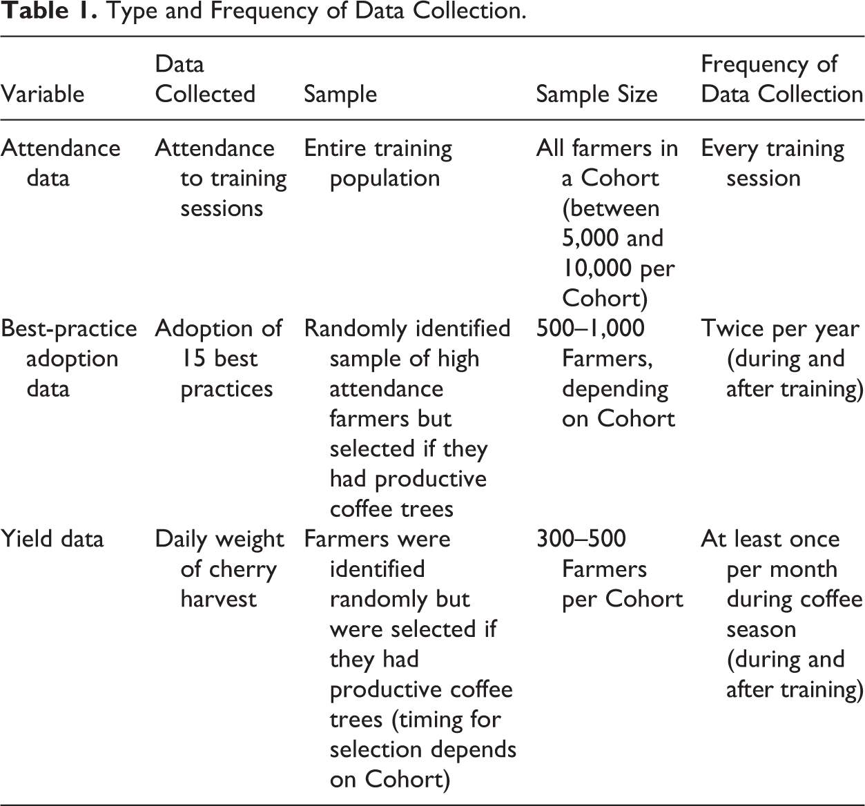
The selection of subgroups by TechnoServe was endogenous to the main sample. Endogenous groups have been used in the evaluation literature to measure the potential effect of no-show rates, different dosages of program quality, different pathways of the program, or different choices by control group individuals when they are denied access to the program (Peck, 2013). In order to adequately select endogenous subgroups for the purpose of evaluation, it is necessary not only to obtain a random sample of the original sample but also to use baseline characteristics to subdivide groups according to the specific evaluation requirements (Peck, 2003; Tipton, 2013). Unfortunately, the endogenous selection of subgroups by TechnoServe did not follow these guidelines. First, TechnoServe randomly identified potential farmers for the yield sample but selected only farmers who had productive coffee trees. ³ For the 2009 and 2010 Cohorts, it is impossible to identify from the sources of information the farmers with unproductive coffee trees who did not meet the inclusion criterion. This is problematic for endogenous subgroup selection. For the 2011 Cohort, data were collected on the number of productive trees from all farmers randomly identified for the yield sample. Therefore, unlike in the case of Cohorts 2009 and 2010, we are able to identify farmers who did meet the additional requirement for selection and we are able to provide more insights into the treatment effects, which we discuss in more detail below. Secondly, TechnoServe collected very little information about the baseline characteristics of farmers, and thus we were unable to verify matching between the three different samples at selection point and potential deviations over time. With the information collected by TechnoServe, we found some differences between the samples in terms of gender composition and cooperative membership. For this reason, we remain cautious about the experimental design and suggest a flexible approach for each of the three Cohorts with the inclusion of controls for estimation purposes.

Low-Frequency With Monitoring of Best-Practices Data Collection

This type of data collection refers to the compilation of best-practice data from a selected group of farmers who we call the best-practice sample. Only farmers who attended 50% of the training sessions during the first year of the program were randomly identified by TechnoServe and then selected into the best-practice sample if the farmer had productive trees. ⁴ Data on best-practice adoption are collected twice per year (starting in Year 2 of the training program): once in the March to June period (Round 1) and once between the months of July to November (Round 2). TechnoServe tracks farmers in the best-practice sample on 11 best coffee-farming practices (record keeping, mulching, weeding, trees nutrition, composting, tree rejuvenation, pruning, safe use of pesticides, Integrated Pest Management [IPM], erosion control, and shade management) and on the use of four types of fertilizers (composting, NPK [Fertilize based on the relative content of the chemical elements Nitrogen (N), Phosphorus (P), and Potassium (K)], Zinc/Borium, and Lime). During the data collection process, a TechnoServe staff member (either a farmer trainer or a data collector) visits a farmer’s plot with a checklist and inspects the farmer’s field, trees, and records. The whole process takes no more than 15–20 min. To assess the update of best practices, staff check whether the farmer has mulched and weeded his or her plot, pruned and rejuvenated the trees, provided enough shade for the trees, taken steps to control erosion, and composted; whether the trees are well nourished; and whether the farmer has kept good records. Then, the staff member asks predetermined questions to test the farmer’s knowledge of IPM and ask the farmer whether he owns the required protection equipment to safely use pesticide and what pesticide he uses. In each Cohort, there are approximately 800 farmers who form the best-practice sample.

High-Frequency With Measurement of Yield and Monitoring of Best-Practices Data Collection

This type of data collection refers to the regular collection of yield and best-practice data from a selected group of farmers who we call the yield sample. As mentioned before, farmers were randomly identified by TechnoServe at the beginning of the program into the yield sample from all farmers who attended the first training session. But only farmers who had productive coffee trees were selected into the yield sample and were provided with weighting scales and log booklets. It is only for the 2011 Cohort that we are able to identify farmers in the original yield sample with and without productive trees (24% of farmers in the yield group had no productive trees and the vast majority of these farmers—or 21% of the farmers initially identified for the yield sample—were not selected to be part of the yield group, as they did not have productive trees to measure yield on that particular year).

Regular collection of data started on the 12th training session for the 2009 Cohort. For the 2010 Cohort, the data collection started on the third training session and for the 2011 Cohort on the second training session. During the coffee season (from March through to August/September), the 300 farmers in the yield sample received monthly visits from TechnoServe staff. They were trained how to use weighting scales to estimate daily coffee production and how to input records into a calendar. On receipt of scales and log booklets, farmers were asked to sign a contract confirming that they had received the scales and committing to keeping daily records on coffee production. Toward the end of each month, TechnoServe staff collected the completed coffee production calendar and provided farmers with a calendar for the subsequent month. In addition to these monthly visits, TechnoServe’s trainers or data collectors visited the coffee farm once per year to survey the number of trees on the farm—thereby enabling the M&E team to calculate yield levels—and once or twice per year to collect information on best-practice adoption. Some plots were also randomly spot checked by TechnoServe business advisors ⁵ to ensure the accuracy of production estimates. This data collection system amounts to regular and structured interactions between project staff and farmers in the yield sample.

The analysis in this article also takes into account who collected the data, since the identity of the data collector is an important factor in program evaluation design. In Cohorts 2009 and 2010, farmer trainers in each cooperative were responsible for collecting attendance, yield, and best-practice data. TechnoServe was criticized for this design, as the trainers themselves, with a stake in the success of the program, were also the ones collecting performance data on their trainees. This led TechnoServe to change the system in 2011, at which point a team of independent enumerators was hired and trained to collect the same information. This break in the data collection system between Cohorts allows us to compare whether the results are significantly different depending on who collected the data.

Estimating Impact on Training Attendance Rates

For all three Cohorts, to estimate the effect of monitoring, we compare the difference in attendance rates between farmers in the yield sample and farmers in the control group using difference-in-differences strategy with the inclusion of controls for cooperative membership and gender of the farmer (Card & Krueger, 1994). For Cohorts 2009 and 2010, where data in the yield sample were only collected for farmers with productive trees only (or compliers), we provide an estimate of the treatment-on-the-treated (TOT) effect (Gertler, Martinez, Premand, Rawlings, & Vermeersch, 2011). As discussed in more detail below, estimates for Cohorts 2009 and 2010 are biased in the favor of the treatment group. For Cohort 2011, where data are available on farmers with both productive and nonproductive trees, we provide an estimate of the intention-to-treat (ITT) effect and an estimate of the local average treatment effect or LATE (Angrist & Imbens, 1994), which is an estimate of the treatment effect on the treated (compliers).

The baseline consists of individual attendance rates in pretreatment training sessions and the end line consists of attendance rates in sessions during or after the data collection period. The length of these periods, both before and during the intervention, varies depending on the Cohort and the sample. The baseline can consist of one or multiple training sessions, as can the treatment itself. This implies that the results we obtain for different Cohorts and samples are not directly comparable, even though in practice, we find that they are quite similar. Because there are multiple time periods in the baseline and treatment, we structure our data as a panel in which each individual session corresponds to a time period. We estimate results using a panel ordinary least squares (OLS) model (Wooldridge, 2010). To ensure robustness, results are also presented using lagged attendance rates as a control in an OLS model (Angrist & Pischtke, 2008).

Formally, we specify this difference-in-differences equation as follows:

Attendance t = β 0 , t + β 1 , t Session t + β 2 , t Treatment + δ 1 , t Session t × Treatment + γ i , t X i + u t ,

Cohorts 2009 and 2010

One key difference in the sample selection for these Cohorts is that the treatment group contains farmers with productive coffee trees only, whereas the control group contains both farmers with and without productive trees. It is likely that farmers with productive trees have different incentives for attending training courses and adopting best practices immediately during the coffee season. This is not the case for farmers whose coffee trees are being rejuvenated, or are otherwise unproductive in a given year, and thus may have fewer incentives to attend the training session regularly. Our inability to differentiate between these groups of farmers implies that any comparison in training attendance rates or best-practice adoption are likely to result in a biased estimate in favor of the treatment group. This estimate is known as the TOT (Gertler et al., 2011).

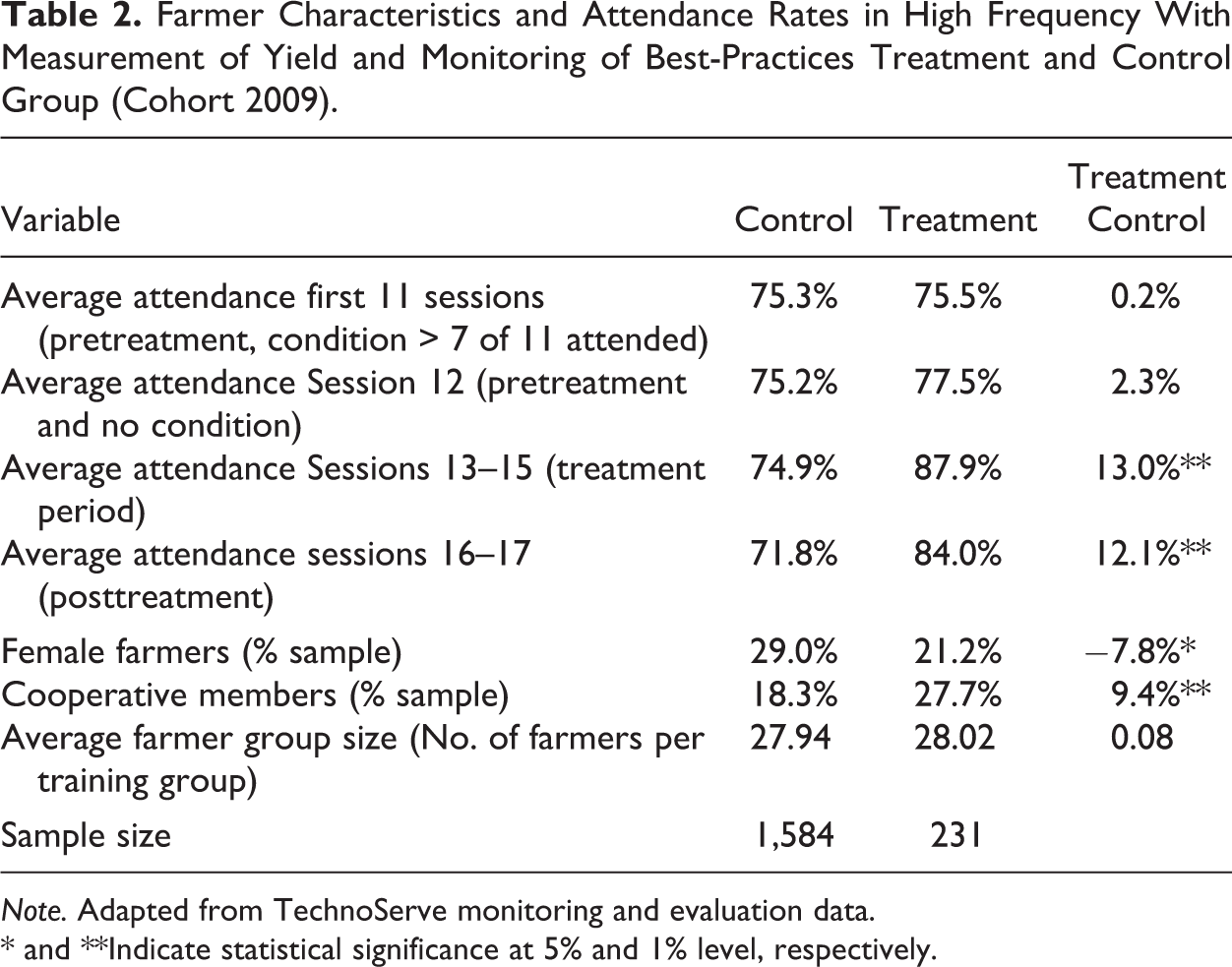
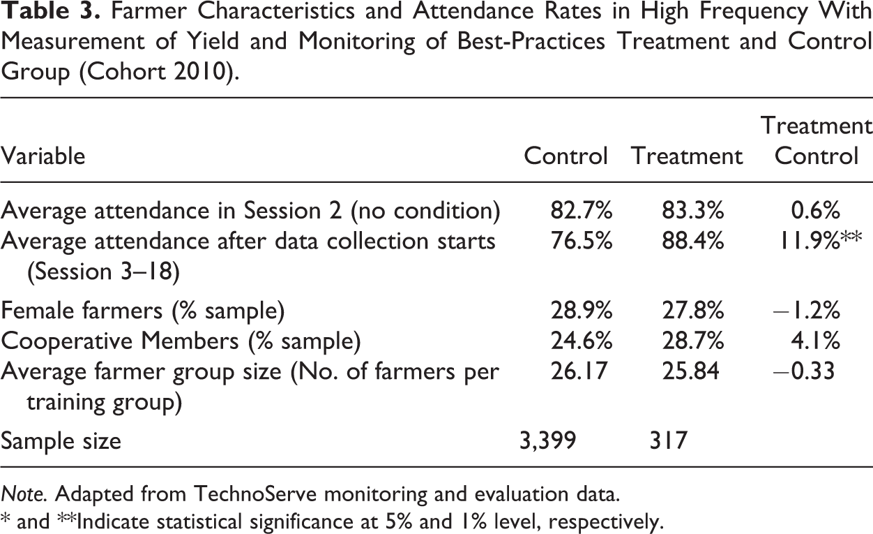
Tables 2 and 3 present evidence of the difference in composition between the yield sample and the control group sample, whereby the yield sample contains more cooperative members in the 2009 and 2010 Cohorts and more male farmers in the 2009 Cohort than the control group. This difference matters for the outcome variable of interest, as on average, cooperative members are more likely to attend training sessions than noncooperative members. Nevertheless, Tables 2 and 3 also show that pretreatment there are no differences in the average training attendance rates for Cohorts 2009 and 2010. In fact, for the Cohort 2009, there are no pretreatment differences for up to 12 months prior to the implementation of the monitoring strategy, hence before the high frequency with measurement of yield and monitoring of best practices, data collection started (see also Figure 1, Panel A).

OPEN IN VIEWER

Table 2.

Farmer Characteristics and Attendance Rates in High Frequency With Measurement of Yield and Monitoring of Best-Practices Treatment and Control Group (Cohort 2009).

Variable	Control	Treatment	Treatment Control
Average attendance first 11 sessions (pretreatment, condition > 7 of 11 attended)	75.3%	75.5%	0.2%
Average attendance Session 12 (pretreatment and no condition)	75.2%	77.5%	2.3%
Average attendance Sessions 13–15 (treatment period)	74.9%	87.9%	13.0%**
Average attendance sessions 16–17 (posttreatment)	71.8%	84.0%	12.1%**
Female farmers (% sample)	29.0%	21.2%	−7.8%*
Cooperative members (% sample)	18.3%	27.7%	9.4%**
Average farmer group size (No. of farmers per training group)	27.94	28.02	0.08
Sample size	1,584	231

Note. Adapted from TechnoServe monitoring and evaluation data.

* and **Indicate statistical significance at 5% and 1% level, respectively.

OPEN IN VIEWER

Table 3.

Farmer Characteristics and Attendance Rates in High Frequency With Measurement of Yield and Monitoring of Best-Practices Treatment and Control Group (Cohort 2010).

Variable	Control	Treatment	Treatment Control
Average attendance in Session 2 (no condition)	82.7%	83.3%	0.6%
Average attendance after data collection starts (Session 3–18)	76.5%	88.4%	11.9%**
Female farmers (% sample)	28.9%	27.8%	−1.2%
Cooperative Members (% sample)	24.6%	28.7%	4.1%
Average farmer group size (No. of farmers per training group)	26.17	25.84	−0.33
Sample size	3,399	317

Note. Adapted from TechnoServe monitoring and evaluation data.

* and **Indicate statistical significance at 5% and 1% level, respectively.

OPEN IN VIEWER

Figure 1.

Attendance rates in treatment and control groups Cohort 2009, 2010, and 2011.

Cohort 2011

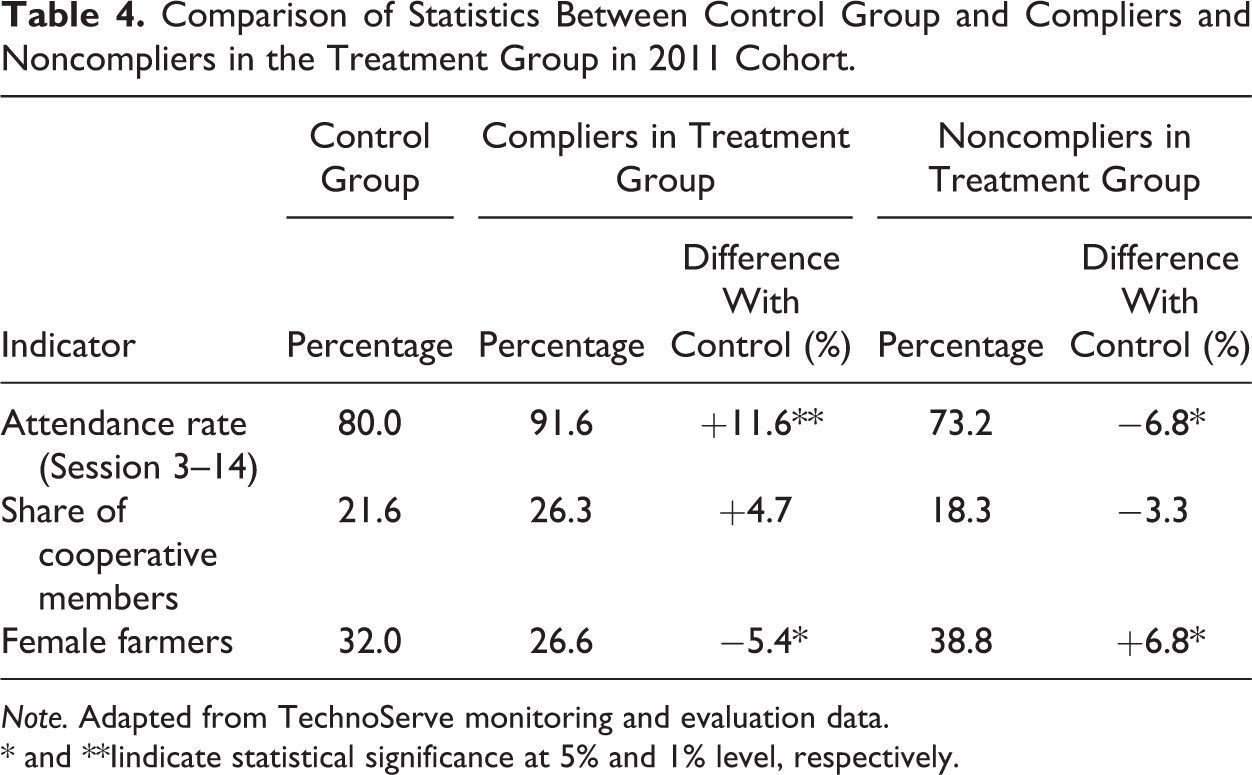
For this Cohort, TechnoServe differentiated between randomly identified farmers in the yield group who had productive coffee trees from those whose coffee trees were being rejuvenated or otherwise unproductive. A direct comparison of training attendance rates and best-practice adoption for farmers with productive trees and those in the control group would again result in an estimate of the TOT which is likely to be biased in favor of the treatment group. The fact that it is possible to identify noncompliers in the Cohort 2011 (or those farmers with nonproductive coffee trees) means that we are able to estimate the ITT effect and thus gain important insights into the size of the bias previously estimated by the TOT effect (Gertler et al., 2011). Table 4 shows differences in the proportion of farmers in each of the treatment groups (compliers vs. noncompliers) with respect to cooperative membership and gender of the farmer. In line with the results from the 2009 and 2010 Cohorts, compliers were more likely to be male farmers and cooperative members than noncompliers.

OPEN IN VIEWER

Table 4.

Comparison of Statistics Between Control Group and Compliers and Noncompliers in the Treatment Group in 2011 Cohort.

Indicator	Control Group	Compliers in Treatment Group		Noncompliers in Treatment Group
	Percentage	Percentage	Difference With Control (%)	Percentage	Difference With Control (%)
Attendance rate (Session 3–14)	80.0	91.6	+11.6**	73.2	−6.8*
Share of cooperative members	21.6	26.3	+4.7	18.3	−3.3
Female farmers	32.0	26.6	−5.4*	38.8	+6.8*

Note. Adapted from TechnoServe monitoring and evaluation data.

* and **Iindicate statistical significance at 5% and 1% level, respectively.

Finally, for all three Cohorts, it is possible to test the robustness of results by comparing attendance rates over time in the yield samples (high-frequency monitoring) versus attendance rates in the best-practice samples (low-frequency monitoring). In both the yield and best-practice samples, farmers who were rejuvenating their trees or had unproductive trees at the time of project implementation were not selected. This is because it is not possible to estimate yields or best-practice adoption if a farmer is not growing coffee in a given year. By comparing attendance rates in the yield and best-practice samples, we therefore circumvent the problem of noncompliance related to the fact that farmers have no productive trees. This comparison results in an underestimation of the actual treatment effect, as we are comparing the high-frequency to low-frequency treatment, as opposed to no treatment.

Estimating Impact on Best-Practice Adoption

It is also possible to test whether high-frequency monitoring—with measurement of yield and monitoring of best practices—is associated with improved agronomic practices by comparing best-practice adoption rates in the yield sample to best-practice adoption rates in the best-practice sample. Our estimate of the treatment effect here is the difference in the impact of high-frequency monitoring (with measurement of yield and monitoring of best-practice data) on best-practice adoption rates versus low-frequency monitoring (with monitoring of best-practices data only). Assuming that the type and frequency of data collection actually affects best-practice adoption rates, this estimate would result in an underestimation of the actual effect of monitoring on best-practice adoption.

While the structure of the data does not enable a difference-in-difference type analysis (there is no pretreatment data on best-practice adoption), for Cohorts 2009 and 2010, it is possible to use panel data to compare the evolution of best-practice adoption rates in the yield and best-practice samples over time, both during and after the end of project activities. For Cohort 2011, only one data point in time is available, during the second year of project implementation. We estimate the difference in best-practice adoption rates between the yield and best-practice samples using a panel OLS model for Cohort 2009 and 2010 and an equivalent least squares regression for Cohort 2011 (Wooldridge, 2010).

Note that in both the yield sample and the best-practice sample, by definition, data are only available for farmers with productive trees. Farmers who were randomly identified to be part of the yield or the best-practice samples and who were rejuvenating their trees or otherwise had unproductive coffee trees at the time of program implementation were excluded from both samples. While we do not face biases here related to the inclusion or not of farmers with unproductive trees, estimates are however biased by the fact that in all three Cohorts, the random selection of the yield and best-practice samples was not done in the same way. Other than in Cohort 2009, where yield farmers were selected among farmers who had participated in at least seven sessions in Year 1 of training, yield farmers in Cohorts 2010 and 2011 were randomly identified at the start of the program among farmers who had participated/registered in training Session 1. Farmers in the best-practice samples on the other hand were selected among farmers who had at least participated in 50% of sessions in Year 1 of training. Had there been no intervention, we would therefore expect best-practice adoption rates to be higher for farmers in the best-practice samples, as they were selected among farmers with a minimum participation rate in Year 1 of 50%.

Farmer Participation in Training: Cohort 2009

For Cohort 2009, we measure the impact of high-frequency data-collection efforts on project attendance rates by comparing the average attendance rate of treatment farmers (farmers in the yield sample with productive coffee trees) in each training session to that of the control group, consisting of all nontreatment farmers who had attended at least eight sessions in Year 1 of training. ⁶ Given that selection was done at the cooperative level (the strata), we ensure that standard errors are clustered by cooperative thus allowing for intragroup correlations and relaxing the usual assumption that observations are independent (White, 1980). We also eliminate focal farmers from the sample, as they have artificially high attendance rates given that the training is conducted in their coffee plots.

Our results show that pretreatment differences between treatment and control groups are negligible in terms of attendance rates. Figure 1, Panel A, depicts attendance rates for the treatment and control groups from Session 1 to the end of the project for the 2009 Cohort. The sessions in Panel A correspond to the period between January 2009 and November 2010. The attendance rates of the treatment and control groups follow almost identical patterns until the beginning of the data collection period in the treatment group, which started in Session 12 (which corresponds to March 2010) and ended after Session 15 (which corresponds to August/September 2010). Attendance rates in the treatment group increased substantially during the intense monitoring period and remained high thereafter.

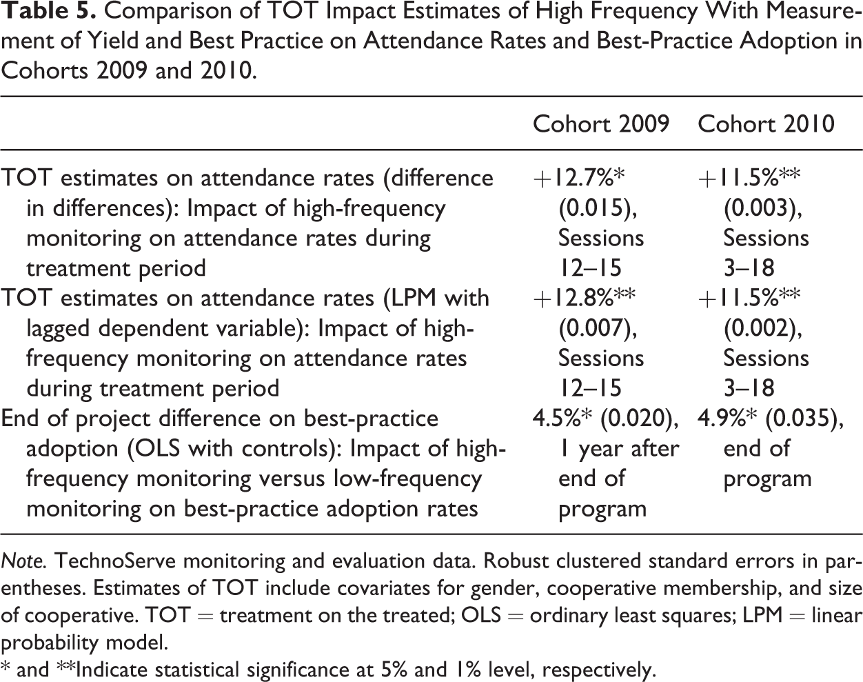
Farmer’s attendance rates, which had been almost identical in both groups before the treatment at an average rate of about 76%, increased to 89.9% in the treatment group during the data collection period but remained unchanged for the control group (see Table 2). These results suggest that the treatment (high frequency with measurement of yield and monitoring of best-practices data collection) led to an increase in farmer attendance rates of about 13 percentage points during the treatment period. Our difference-in-differences estimate of the TOT with the inclusion of controls is 12.7 percentage points and is statistically significant at the 1% level (see Table 5). The results using the OLS model with lagged dependent variable as control show an impact of 12.8 percentage points, also statistically significant at 1% level (see Table 5).

OPEN IN VIEWER

Table 5.

Comparison of TOT Impact Estimates of High Frequency With Measurement of Yield and Best Practice on Attendance Rates and Best-Practice Adoption in Cohorts 2009 and 2010.

	Cohort 2009	Cohort 2010
TOT estimates on attendance rates (difference in differences): Impact of high-frequency monitoring on attendance rates during treatment period	+12.7%* (0.015), Sessions 12–15	+11.5%** (0.003), Sessions 3–18
TOT estimates on attendance rates (LPM with lagged dependent variable): Impact of high-frequency monitoring on attendance rates during treatment period	+12.8%** (0.007), Sessions 12–15	+11.5%** (0.002), Sessions 3–18
End of project difference on best-practice adoption (OLS with controls): Impact of high-frequency monitoring versus low-frequency monitoring on best-practice adoption rates	4.5%* (0.020), 1 year after end of program	4.9%* (0.035), end of program

Note. TechnoServe monitoring and evaluation data. Robust clustered standard errors in parentheses. Estimates of TOT include covariates for gender, cooperative membership, and size of cooperative. TOT = treatment on the treated; OLS = ordinary least squares; LPM = linear probability model.

* and **Indicate statistical significance at 5% and 1% level, respectively.

Interestingly, the monitoring effect persists even after the end of the treatment period. While average attendance rates in the treatment group dropped by a full 3.9 percentage points between Sessions 15 and 16—that is, between August and September 2010 when the coffee season and the “yield data” collection period came to an end—they nevertheless remained about 12 percentage points higher than in the control group. Average attendance rates in the last two sessions of the project, held between September and December 2010, were 84% in the treatment group compared to just 71.8% in the control group. This suggests that 7 months of data collection, from March 2010 through to August 2010, had effects on average attendance rates in the treatment group for at least 4 months after the end of the data collection period.

Note, as explained in the Method section, that these estimates on Cohort 2009 are likely to overestimate the effect of high-frequency monitoring on attendance rates as farmers who were rejuvenating their coffee tree or otherwise had unproductive trees at the time of project implementation were removed from the “yield” sample. These farmers, who in all likelihood do not have as many incentives to regularly participate in the program, are nevertheless still included in the control sample, leading to an overestimation of the actual treatment effect. The problem is that we do not know how many farmers do not have productive trees, which makes it difficult to estimate the size of the bias.

Farmer Participation in Training: Cohort 2010

The link between regular and structured data collection efforts and farmer attendance levels is confirmed using attendance data from the 2010 Cohort. In the 2010 Cohort, farmers in the yield sample were randomly identified among farmers who had attended Session 1 of the training program, but only those with productive coffee trees were selected for monitoring yields. ⁷ The control group consists of all nontreatment farmers in Cohort 2010 who also attended Session 1 of the training program (including farmers with and without productive coffee trees at the time of selection). Data collection on yield levels in Cohort 2010 started in Session 3 of the program, which corresponds to the month of March 2010 (Figure 1, Panel B). High-frequency data collection covered the May to June periods in both years of the training program (which corresponds to Sessions 3–6 of the project in Year 1 and Sessions 12–14 in Year 2).

As in the case of Cohort 2009, we find that the initial attendance rates of the treatment and control groups for the Cohort 2010 are relatively similar. In particular, we cannot reject the null hypothesis that pretreatment or baseline attendance rates in Session 2 were the same in the treatment and control groups. As in the case of Cohort 2009, we do find differences in terms of cooperative membership and gender between treatment and control, but these are not statistically significant (see Table 3).

Once the regular data collection of the treatment group started in Session 3 in March 2010, attendance rates increased significantly in the treatment group, from 83.3% in Session 2 to an average of 88.4% for the remaining sessions of the project. For the control group, however, attendance rates declined from 82.7% in Session 2 to an average of 76.5% for the remaining sessions of the project. Attendance rates in the treatment group were therefore on average about 12 percentage points higher than in the control group throughout the remainder of the 2-year program, which covered two separate coffee seasons (see Figure 1, Panel B). Our difference-in-difference estimate of the TOT with controls is 11.5 percentage points and is statistically significant at the 1% level (see Table 5). The point estimate is also 11.5 percentage points using an OLS model with lagged dependent variable as control and remains statistically significant. Note that, as in the case of Cohort 2009, these estimates are likely to be an overestimation of the actual treatment effect, as farmers who did not have productive trees were dropped from the treatment group (we do not have a record of which farmers these were) but not from the control group.

Based on the evolution of relative attendance rates in the treatment and control groups over time, we can derive the following two properties about the monitoring effect in the case of TechnoServe’s Coffee Agronomy program in Rwanda:

The monitoring effect persists for several months beyond the treatment period. For the 2010 Cohort, for example, data collection stopped in September 2010, but the effect was still present and growing in January 2010, 4 months later. The difference between the treatment and control groups even increased between data collection periods in Cohort 2010 because attendance rates dropped less in the treatment group than in the control group (see Figure 1, Panel B).

Farmers With Low Participation in Training: Cohorts 2009 and 2010

Our results also show that the effect of the high-frequency monitoring of yield and best-practice data lifts the participation levels of low-attendance farmers the most, both in Cohorts 2009 and 2010 (Figure 2, Panels A and B). In the control samples of both Cohorts 2009 and 2010, we find a very strong linear correlation between participation rates in Year 1 and in Year 2 of the program: Farmers with high participation levels in Year 1 also had high participation levels in Year 2, while farmers with low participation levels in Year 1 had low participation levels in Year 2. The treatment changes the dynamics of this association. High-participation farmers in Year 1 remained high-participation farmers in Year 2 after the treatment, which could in part be the result of a sustaining benefit of the monitoring strategy. Low-participation farmers, who would otherwise have remained low-participation farmers in the absence of treatment, also became high-participation farmers in Year 2, which we interpret as being a transforming benefit of the monitoring strategy. The treatment effect on attendance levels disappears for farmers with high initial attendance levels but increases exponentially for farmers with low participation levels. In Cohort 2009 (Figure 2, Panel A), for example, farmers who had attended only eight sessions in Year 1 saw their Year 2 attendance rates increase by 39%, compared to just 3% for farmers who had attended 11 sessions in Year 1. Note that the difference for Cohort 2009 is the actual treatment effect on the treated as we are comparing average attendance rates after the intervention (i.e., after Session 12), with attendance rates before the intervention. This is not the case for Cohort 2010 (Figure 2, Panel B), where the intervention started in Session 3.

OPEN IN VIEWER

Figure 2.

Difference in attendance rates based on attendance in Year 1: Cohorts 2009, 2010, and 2011.

Farmer Best-Practice Adoption Rates: Cohorts 2009 and 2010

Best-practice adoption rate is measured by the share of the number of best coffee-farming practices adopted (maximum 11). In both Cohorts 2009 and 2010, we find that farmers in the yield sample (treatment) performed significantly better than farmers in the best-practice sample on best-practice adoption rates over time (control). The best-practice adoption rates among farmers in the yield sample were on average 4.9 percentage points higher in the 2009 Cohort and 4.5 percentage points higher in the 2010 Cohort compared to farmers in the best-practice sample after controlling for individual characteristics, group size, and cooperative membership (see Table 5). Although farmers in the yield sample had significantly higher average attendance rates overall than farmers in the best-practice sample (see comparison of attendance rates in yield and best-practice samples in section below), the treatment effect shown in Table 5 does not disappear when keeping farmer attendance rates constant in both Cohorts. These findings present evidence that best-practice adoption rates could be directly affected by the more intense face-to-face interactions between beneficiaries and trainers imposed by the high-frequency monitoring strategy. It is possible that these interactions could have led to more personalized advice for beneficiaries or simply nudged farmers to implement what they had learned as in the Hawthorne effect. ⁸

ITT and the Identity of the Data Collector: Cohort 2011

So far, we have provided insights into the effects of the monitoring strategy using the 2009 and 2010 Cohorts. However, as mentioned before, having only farmers who comply with the treatment implies that we are potentially overestimating the monitoring effect. The 2011 Cohort enables the estimation of the ITT using data from farmers who were randomly identified to be part of the yield sample but later excluded as they did not have productive coffee trees. By including noncomplier farmers as part of the treatment group, we are estimating the ITT and thus adjusting for the bias previously estimated by the TOT. Furthermore, we use results from Cohort 2011 to test whether the monitoring effect holds when yields and best-practice data are collected by independent enumerators. There are inherent differences in the dynamics of the interaction between farmers and the farmer trainer, who delivers the training sessions, has in-depth knowledge about coffee farming, and has a stake in his farmers doing better, versus independent enumerators. We would expect farmers to feel greater pressure to attend training sessions and implement best practices after repeated visits by their trainer. We would also expect them to benefit more from the face-to-face interaction with someone who can advise them on their farming practices.

For the 2011 Cohort, Figure 1, Panel C, confirms that farmers who were assigned to the yield sample in Session 1 of the program had significantly higher attendance rates afterward than farmers who were not assigned to the yield sample. The case of Cohort 2011 is slightly more complicated analytically, as monitoring had already partially started between Sessions 1 and 2 of the program, potentially leading to the difference in attendance rates observed in Session 2 of the program. This difference might also reflect selection bias in the yield sample. We nevertheless use Session 2 as a pretreatment period in the difference-in-difference analysis. In addition, as was the case in Cohorts 2009 and 2010, Figure 2, Panel C, confirms that attendance in the second half of the program increases more for farmers who started with a lower base in terms of their attendance in the first half of the program.

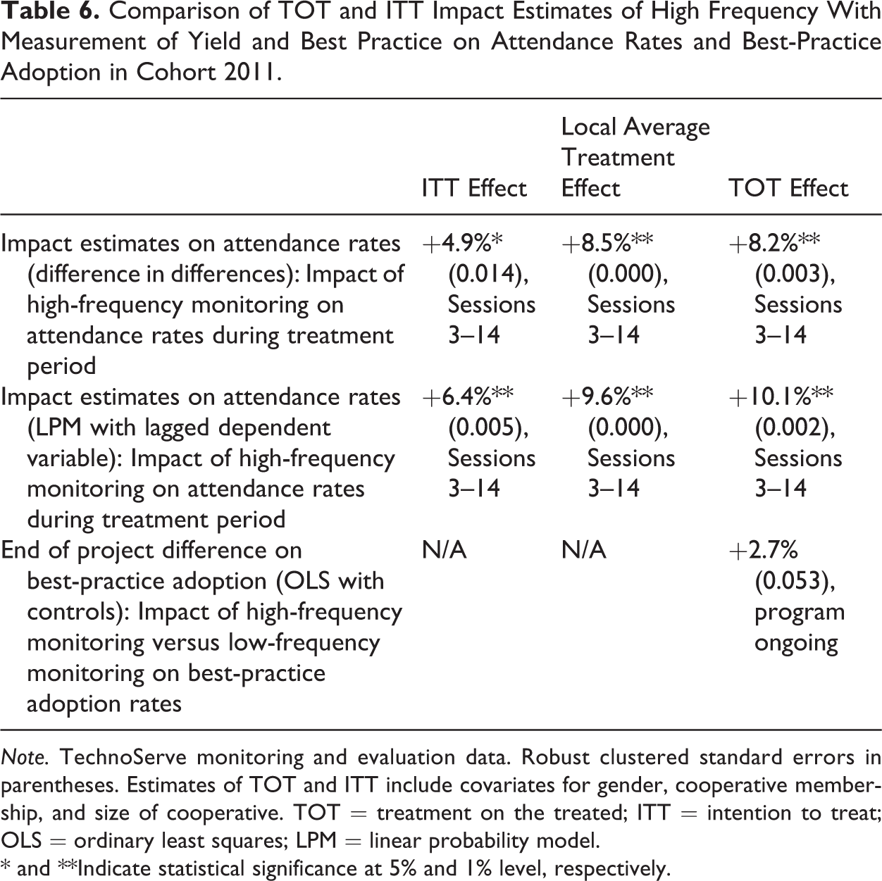
Finally, results shown in Table 6 provide evidence on the ITT versus the TOT and LATE estimates. For the 2011 Cohort, if we were to measure the TOT in a similar way to Cohorts 2009 and 2010—that is, including only compliers in the treatment sample—we would obtain an estimated TOT of 8.2 percentage points on attendance rates estimated using difference in differences. The ITT in this case—including in the treatment sample the 21% of treatment farmers who were not treated—is 4.9 percentage points. Using an instrumental variables approach following Angrist and Imbens (1994)—where the instrument is the assignment or not to the treatment group and the instrumented variable is whether or not farmers complied to the treatment (i.e., received the treatment)—it is possible to calculate the LATE, which is an estimate of the treatment effect on compliers. The LATE in this case would be 8.5 percentage points, which is highly comparable to the TOT estimate of 8.2 percentage point, suggesting that in the case of Cohort 2011, the TOT does not provide a very large overestimation of the treatment effect on the treated.

OPEN IN VIEWER

Table 6.

Comparison of TOT and ITT Impact Estimates of High Frequency With Measurement of Yield and Best Practice on Attendance Rates and Best-Practice Adoption in Cohort 2011.

	ITT Effect	Local Average Treatment Effect	TOT Effect
Impact estimates on attendance rates (difference in differences): Impact of high-frequency monitoring on attendance rates during treatment period	+4.9%* (0.014), Sessions 3–14	+8.5%** (0.000), Sessions 3–14	+8.2%** (0.003), Sessions 3–14
Impact estimates on attendance rates (LPM with lagged dependent variable): Impact of high-frequency monitoring on attendance rates during treatment period	+6.4%** (0.005), Sessions 3–14	+9.6%** (0.000), Sessions 3–14	+10.1%** (0.002), Sessions 3–14
End of project difference on best-practice adoption (OLS with controls): Impact of high-frequency monitoring versus low-frequency monitoring on best-practice adoption rates	N/A	N/A	+2.7% (0.053), program ongoing

Note. TechnoServe monitoring and evaluation data. Robust clustered standard errors in parentheses. Estimates of TOT and ITT include covariates for gender, cooperative membership, and size of cooperative. TOT = treatment on the treated; ITT = intention to treat; OLS = ordinary least squares; LPM = linear probability model.

* and **Indicate statistical significance at 5% and 1% level, respectively.

We find similar results using the OLS model with the lagged dependent variable. In this case, the LATE on attendance rates for the 2011 Cohort is 9.6 percentage points and the TOT is 10.1 percentage points, whereas the ITT is 6.4 percentage points. Again, the difference between the LATE and the TOT estimation is relatively small of the order of 0.5 percentage points.

For best-practice adoption rates, we found an increase in best-practice adoption of 2.7 percentage points for the 2011 Cohort. The point estimate is not as high as the one estimated for the 2009 or 2010 Cohorts. This may be due to differences in measurement of what constitutes a best-practice between independent enumerators and farmer trainers. It may also be that farmers in the 2011 Cohort were still in the program and the adoption of best practices takes longer time. In any case, the point estimate for the 2011 Cohort remains statistically significant at the 10% level (p value = .053), indicating that higher frequency interactions between enumerators and farmers appears to be strongly associated with an increase in best-practice adoption rates.

Comparing the Effect of High-Frequency Versus Low-Frequency Monitoring on Attendance Rates: All Cohorts

Another way to test whether the exclusion of farmers without productive trees in Cohorts 2009 and 2010 led to a large overestimation of impact estimates is to compare attendance rates over time in the yield (or high-frequency monitoring) and “best-practice” (or low-frequency monitoring) samples. A comparison of attendance rates in the high-frequency versus low-frequency monitoring samples would lead to an unbiased estimation of the effect of higher frequency monitoring on attendance rates in so far compliance is concerned. We estimate this effect for all three Cohorts adopting an equivalent difference-in-difference approach to the one used previously. The only difference is that instead of the control group being composed of farmers who were not included in the yield sample, here the control group is composed of farmers who were included in the best-practice sample and not in the yield sample.

Note that the estimates resulting from this analysis will constitute an underestimation of the actual treatment effect of monitoring on attendance rates for two reasons: (i) here, we are comparing high-frequency versus low-frequency monitoring, as opposed to high-frequency monitoring versus no- and/or low-frequency monitoring and (ii) the best-practice samples were selected among high-participation farmers (farmers who had attended at least 50% of sessions), whereas yield sample farmers were selected among farmers who had participated in Session 1 of the program. The only exception is Cohort 2009, where both the yield and best-practice samples were selected among high-participation farmers, which might explain why we find a higher point estimate in the results below for Cohort 2009, compared to Cohorts 2010 and 2011.

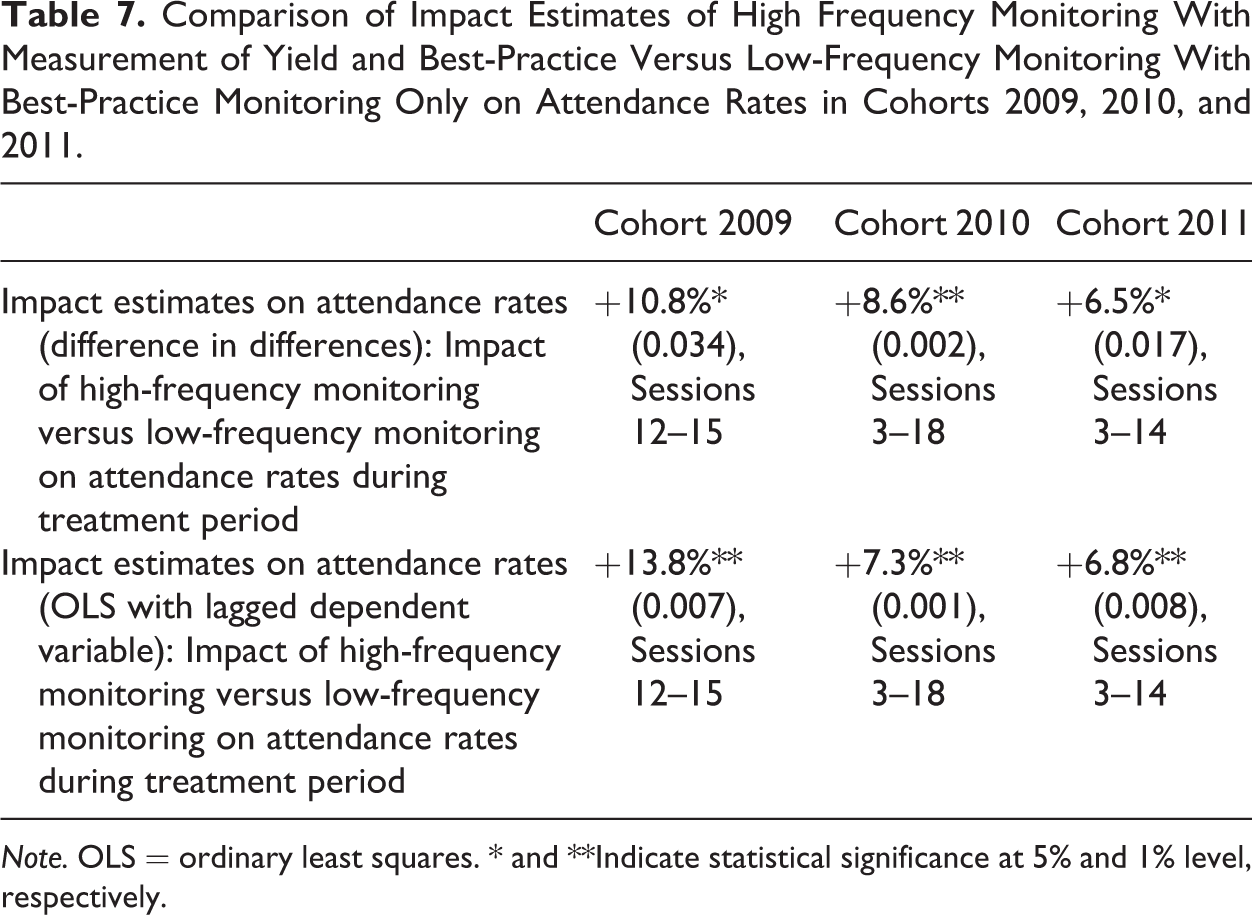
Results shown in Table 7 for all three Cohorts are summarized below:

OPEN IN VIEWER

Table 7.

Comparison of Impact Estimates of High Frequency Monitoring With Measurement of Yield and Best-Practice Versus Low-Frequency Monitoring With Best-Practice Monitoring Only on Attendance Rates in Cohorts 2009, 2010, and 2011.

	Cohort 2009	Cohort 2010	Cohort 2011
Impact estimates on attendance rates (difference in differences): Impact of high-frequency monitoring versus low-frequency monitoring on attendance rates during treatment period	+10.8%* (0.034), Sessions 12–15	+8.6%** (0.002), Sessions 3–18	+6.5%* (0.017), Sessions 3–14
Impact estimates on attendance rates (OLS with lagged dependent variable): Impact of high-frequency monitoring versus low-frequency monitoring on attendance rates during treatment period	+13.8%** (0.007), Sessions 12–15	+7.3%** (0.001), Sessions 3–18	+6.8%** (0.008), Sessions 3–14

Note. OLS = ordinary least squares. * and **Indicate statistical significance at 5% and 1% level, respectively.

These findings confirm that the exclusion from the yield sample of farmers without productive coffee trees cannot fully explain the observed impact of high-frequency monitoring on attendance rates. On the contrary, high-frequency monitoring appears to lead to significantly higher participation rates even when compared to farmers who were exposed to low-frequency monitoring and that were selected among high-participation farmers to start with.

The consistency of the impact estimates in all three Cohorts conflict with two potential explanations of the monitoring effect:

The possibility that the monitoring effect is primarily due to the face-to-face transfer of knowledge transfer that occurs when the farmer meets the project staff and in particular the farmer trainer himself; and

While we cannot identify the transmission mechanism, alternative and potentially more likely explanations of the monitoring effect include:

The possibility that the presence of data collectors serves as a “reminder” to farmers that they need to attend training sessions and implement certain best practices; or

Concluding Remarks

In this article, we show that the monitoring strategy can significantly alter the behavior and engagement levels of project beneficiaries and serve as an effective tool to improve project outcomes. In the particular case of TechnoServe’s Coffee Agronomy program in Rwanda, we show that intensive monitoring for measuring yield and best practices led to better outcomes through two parallel channels: (i) it affected farmer attendance to training which in turn could have led to better best-practice adoption rates and (ii) it affected best-practice adoption rates directly possibly because it served as a reminder to farmers or because it gave farmers the extra “nudge” that was needed to implement what they had learned in class.

Second, we found that the monitoring effect lasts beyond the treatment period. Our results are in line with other similar studies. For example, Dhokolakia and Morwitz (2002) found that the effect of measuring consumer satisfaction increases for several months after surveying and can persist a year later. Zwane et al. (2011) also found long-lasting effects of surveying on respondents’ behaviors. Third, we found that the monitoring effect was greater for low-attendance farmers. Finally, we posit that the monitoring effect operates either as a Hawthorne and John Henry effects, whereby beneficiaries and control group derive motivation from more face-to-face interaction with M&E staff, or as a reminder effect, whereby data collection serves as a reminder to farmers who they need to attend training sessions and implement certain best practices.

It is important to highlight that what we have called in this article the “monitoring effect” amounts to more than simply surveying households with different degrees of intensity, as it is the case of other studies such as Cantor (2008) and Zwane et al. (2011) but encompasses regular and structured interactions for data collection. Therefore, one could say that the monitoring effect here is more than the “survey effect,” as we are capturing aspects of the program only given to the high-frequency group.

There are important limitations to our study. First, our empirical estimation uses different clusters of time periods for the period of high-frequency data collection. For the 2009 Cohort, we used 4 time periods; whereas for the 2010 and 2011, we used more than 10 time periods. Given the possibility of decreasing effects over time, and the fact that data on attendance rates were only collected during the coffee seasons, our point estimates may not be capturing the full picture of the monitoring effect. Secondly, to understand the impact of best-practice adoption, it is important to know if farmers in Rwanda face knowledge gaps, economic, or cultural barriers to best-practice adoption. If could be that under economic or cultural barriers, the monitoring effect may not operate in the same way as if farmers face a knowledge gap. Lastly, our point estimates for the monitoring effect are not isolated from other potential influences, both observed (such as other programs operating with farmer’s cooperatives) and unobserved (such as farmers motivations) which can impact on farmer’s behavior and thus on the estimation of parameters. To some extent, we captured some of these biases with an estimate of the ITT.

We also highlighted similar patterns of participation in training and best-practice adoption between farmers in the treatment group and those in the control group prior to the intense period of monitoring. This important issue suggests common trends prior to the intervention which is an important condition for obtaining unbiased estimates using difference in differences (Gertler et al. 2011). In addition, this evidence suggested that indeed deviations from common practice took place during the period of intense monitoring and not before.

Notwithstanding these limitations, our findings have a number of important implications for project design and for program evaluation. In terms of project design, the main point we want to put across is that data collection should not only be used as an independent tool to evaluate the effectiveness of a given development program and to keep track of project performance indicators but as an active intervention to improve project outcomes and the engagement levels of beneficiaries. Few development projects (except large-scale interventions) have extensive monitoring mechanisms in place because evaluation is still perceived as an expensive obligation that mainly serves reporting purposes and that only needs to happen at the very beginning and end of a project to show evidence of impact (baseline and end line). However, as we show, the frequency and type of data collection not only provides more data and a better understanding of project dynamics (which in turn can help improve design) but can also improve project outcomes in particular for the least engaged. The additional impact on outcomes due to monitoring could well justify the cost.

If cost however remains too big a barrier to make extensive monitoring within a given project feasible, project designers could consider a number of alternatives, for example, only targeting beneficiaries who are expected to be the least engaged in the program. At least in this case, the TechnoServe’s agronomy program seemed to disproportionately affect farmers with low levels of participation. Another important aspect of our research, which remains unexplored, is whether there could be ways to also achieve the impact of monitoring through less expensive means of data collection, for instance, with the use of mobile devices.

The monitoring effect also has important implications for program evaluation. If this study has external validity—and similar findings in the literature suggest this might be the case (McCarney et al., 2007; Zwane et al., 2011)—it would imply that in many impact evaluations, we have been overestimating the average impact of development interventions, especially in the cases where high-intensity interactions occur between project leaders and project participants. The monitoring effect, which as we show here is nonnegligible, introduces a bias because it doesn’t affect beneficiaries in the treatment and control groups in the same way. To illustrate this point, consider the case where we collect data on coffee farmers who are part of the agronomy program (the treatment group) and compare them to a similar group of farmers who are not part of the program (the control group). The evaluation, which serves as a reminder or an extra nudge for farmers in the treatment group, would lead them to attend more and implement the best practices they learned; it would not and cannot have the same effect on farmers in the control group, for the simple reason that they have not been exposed to the best practices in question. While the effects might be negligible if the evaluation happens at the very beginning and end of the program, they are probably not negligible if multiple interactions between beneficiaries and data collectors take place.

Program evaluation therefore needs to take into account the expected consequences of monitoring. Given that some form of evaluation is needed to obtain the necessary data, fully controlling for the impact of monitoring is virtually impossible. However, by properly assigning beneficiaries in the treatment and control groups to different forms of monitoring, as suggested by Peck (2003, 2013), researchers can gain a better understanding of how monitoring is affecting project outcomes and adjust impact estimates accordingly.