RD or Not RD: Using Experimental Studies to Assess the Performance of the Regression Discontinuity Approach

Abstract

Background:

This article explores the performance of regression discontinuity (RD) designs for measuring program impacts using a synthetic within-study comparison design. We generate synthetic RD data sets from experimental data sets from two recent evaluations of educational interventions—the Educational Technology Study and the Teach for America Study—and compare the RD impact estimates to the experimental estimates of the same intervention.

Objectives:

This article examines the performance of the RD estimator with the design is well implemented and also examines the extent of bias introduced by manipulation of the assignment variable in an RD design.

Research design:

We simulate RD analysis files by selectively dropping observations from the original experimental data files. We then compare impact estimates based on this RD design with those from the original experimental study. Finally, we simulate a situation in which some students manipulate the value of the assignment variable to receive treatment and compare RD estimates with and without manipulation.

Results and conclusion:

RD and experimental estimators produce impact estimates that are not significantly different from one another and have a similar magnitude, on average. Manipulation of the assignment variable can substantially influence RD impact estimates, particularly if manipulation is related to the outcome and occurs close to the assignment variable’s cutoff value.

Keywords

methodological development content area quasi-experimental design methodology (if appropriate)outcome evaluation (other than economic evaluation)design and evaluation of programs and policies education

A key challenge in the field of program evaluation is to develop study designs that can generate unbiased and/or statistically consistent estimates of program or intervention impacts in cases in which an experimental design is not possible. Regression discontinuity (RD) designs have become popular alternatives in such situations (Chiang, 2009; Jacob & Lefgren, 2009; Moss, Yeaton, & LIoyd, 2014; Niu & Tienda 2010; Van der Klaauw, 2002). An RD design can be used when the mechanism for determining who participates and who does not participate in a program is known and is based on the value of a single variable (or small set of variables) known as an assignment variable. While RD designs have appealing theoretical properties (Hahn, Todd, & Van Der Klaauw, 2001; Imbens & Lemieux 2008), questions remain about the performance of RD estimators in empirical applications.

We explore the performance of RD designs for measuring program impacts using a synthetic within-study comparison (WSC) design. WSCs assess quasi-experimental designs by comparing their causal estimates to those from an experimental design when the experiment and quasi-experiment share the same treatment group (Cook, Shadish, & Wong, 2008). In a synthetic WSC, the quasi-experimental data are generated artificially in some way from the experimental data (Wong & Steiner, 2018). We compare experimental and synthetic RD estimates using data from two recent experimental evaluations of educational interventions—the Educational Technology (Ed Tech) study (Dynarski et al., 2007) and the Teach for America (TFA) study (Decker, Mayer, & Glazerman, 2004). We also examine whether different RD estimation methods—parametric and nonparametric—yield estimates that are more or less likely to match the experimental estimates. In addition, we examine the sensitivity of the results to alternative scenarios involving manipulation of the assignment variable, whereby a program’s applicants or program operators alter the values of the assignment variable for some applicants in order to ensure that they are (or are not) admitted to the program.

This study makes three important contributions to the WSC literature on the validity of RD designs. First, the study provides an additional replication to prior WSCs that have shown the RD designs yield estimates of program impacts similar to those generated by experimental designs (e.g., Black, Galdo, & Smith, 2007; Buddelmeyer & Skoufias, 2004; Green, Leong, Kern, Gerber, & Larimer, 2009; Shadish, Galindo, Wong, Steiner, & Cook, 2011; Tang & Cook, 2018; Tang, Cook, & Kisbu-Sakarya, 2015; Wing & Cook, 2013). Because the performance of RD methods can vary based on the context of the study in which they are being used, replicating their ability to reproduce experimental estimates through WSCs is useful. Second, this study addresses the limited statistical power that many comparisons of RD and experimental estimates face by combining in a meta-analytic style multiple estimates of the RD–experimental difference across studies (interventions), subjects, and approach to simulating the RD data. This allows us to assess the performance of parametric and nonparametric RD models. Third, the study produces evidence on the diagnostic value of a test for the presence of manipulation of the assignment variable in RD designs. By simulating the presence of manipulation, we are able to address one of the inherent limitations of synthetic WSCs of RD designs—that in creating the synthetic RD design, the standard approach implicitly assumes no manipulation of the assignment variable.

Our synthetic WSC allows us to compare RD and experimental impact estimates of the same intervention even though actual assignment to treatment was experimental and not implemented in a way that would ordinarily allow for an RD design. The centerpiece of the approach is the construction of synthetic RD analysis files, by selectively dropping observations from the original experimental data files. Specifically, we selected a baseline characteristic (a pretest score) from the original study as the assignment variable and a cutoff value (the median) for this assignment variable. Because assignment to treatment status was random, the distribution of the assignment variable is independent of treatment status; that is, its distribution is identical for treatment and control group members. We then dropped all treatment group members with values of the assignment variable on one side of (below) the threshold and all control group members on the other side of (above) the threshold. The resulting data set mimics a situation in which treatment status is determined solely by the value of the assignment variable and an RD design would be appropriate.

The resulting data set, which we call RD high, matches one that would have resulted if treatment status had been assigned based on having a value of the assignment variable above the median. For example, a school district may have decided that a particular intervention was most appropriate for students in the top half of the achievement distribution, and thus assigned students whose prior test scores were above the median to intervention classrooms and those with below-median scores to control classrooms. We repeated this process to construct an RD low data set where we kept treatment students with values of the assignment variable below the median and control students with values above the median and used sharp RD to estimate impacts at the cutoff value.

A key limitation of a WSCs—whether synthetic or not—that compare RD and experimental estimates is that the two methods estimate different causal estimands. Experimental designs typically produce an average treatment effect (ATE) over a range of values of the assignment variable and RDs produce the estimated impact at a particular value of the assignment variable. To address this difference, we generated experimental impacts using a limited range of values of the assignment variable that surround the RD cutoff value.

As noted by Wong and Steiner (2018), the fact that our WSC is synthetic leads to another key limitation. In the real world, there can be implementation problems that are difficult or impossible to observe but that may lead to bias, while the synthetic approach implicitly assumes perfect implementation—that is, all cases on one side of the threshold get the intervention and all cases on the other side do not, and no one manipulates any values of the assignment variable. This is an important issue, but the usual synthetic WSC approach assumes it away. To shed light on this issue, we simulated different forms of manipulation of the assignment variable to test how RD analytical methods are affected by manipulation. We examine whether the presence of manipulation leads to bias in the impact estimate and whether one example of a test for the presence of manipulation successfully detects it.

We find that in the context of these two education interventions, the RD designs produce impact estimates that closely match those of the experimental benchmark, after accounting for sampling variability. This was true for both the parametric and nonparametric RD specifications. We also find that a test for the presence of manipulation of the assignment variable in RD designs has good diagnostic properties—in simulations, it consistently detects bias due to manipulation that is moderate or high in magnitude.

Study Design

We implemented this replication study using data from the recent Ed Tech Study (Dynarski et al., 2007) and the TFA Study (Decker et al., 2004).

Ed Tech Study

The Ed Tech study was designed to examine whether education technology in the classroom leads to higher student achievement, as called for by the No Child Left Behind Act of 2002. The study used an experimental design to estimate the impact of reading and mathematics software products on test scores among elementary and secondary school children, covering four subjects—Grade 1 reading, Grade 4 reading, Grade 6 math, and high school algebra. We used first year follow-up data from the Ed Tech study to conduct this replication exercise.

In the original Ed Tech study, teachers within a given school and grade were randomly assigned either to a treatment group, where they would implement one of the products in their classroom, or to a control group, where they did not receive the product.¹ Students were tested at the beginning and end of the 2004–2005 school year, the year in which the products were in place. Impact estimates were based on differences in end of year, or posttest, scores for the students in treatment classrooms compared to students in control classrooms.

Data from the Ed Tech study are appropriate for this replication exercise for several reasons. The study employed a straightforward random assignment process, resulting in a large student sample—9,424 students in the classrooms of 439 teachers in 132 schools and 33 districts. The experiment was well implemented, with no significant differences in the mean baseline characteristics of the treatment and control groups (Dynarski et al., 2007). The baseline test administered to the student sample provides a good candidate for the assignment variable in our RD analysis. One might imagine an intervention being provided only to the lowest performing students, with performance on a standardized test used to determine students’ eligibility for the intervention.

We used a subset of the original Ed Tech data in the current study, pooling data from Grades 1, 4, and 6. We used these three grades because they all used a common test—the Stanford Achievement Test—and were normed to a common scale. Our final Ed Tech analysis sample for the RD replication exercise consisted of 7,569 students and 355 teachers. The data were weighted to account for nonresponse and unequal probabilities of assignment to treatment.

TFA Study

TFA was founded in 1989 to address the educational inequities facing children in low-income communities by expanding the pool of teacher candidates available to the schools those children attend. The TFA study examined the impact of TFA teachers on students in their classrooms, compared with what would have happened in the absence of the TFA teachers (Decker et al., 2004). To ensure the comparability of students in TFA classrooms and students in non-TFA classrooms, the study randomly assigned students to classrooms before the start of the school year. The random assignment of students was conducted within school and grade-level blocks. The final analytic sample included 1,765 students in 37 random assignment blocks across 17 schools.

As part of the study, students completed the Iowa Test of Basic Skills as a pretest in the fall and a follow-up posttest in the spring. The data were weighted to account for nonresponse and unequal probabilities of assignment to treatment. The analysis of baseline data suggested that random assignment was successful, with no significant demographic or baseline achievement differences between students in the treatment and control classrooms (Decker et al., 2004).

Estimating Impacts Using an RD Design

We estimated the impacts of the Ed Tech and TFA interventions using both parametric and nonparametric RD approaches. The basic parametric approach involved modeling the outcome test, or posttest, score as a function of the pretest score (the assignment variable) and treatment status. We estimated the following model:

y_{i j} = α_{0} + α_{1} T_{i j}^{RD} + m (δ, Z_{i j}) + X_{i j} α_{2} + η_{j} + ∊_{i j},

where y_ij is the outcome test score of student i in classroom j, T_ij is a treatment indicator, Z_ij is the pretest score, m(δ, Z_ij ) is a function of the pretest score and a vector of parameters, X_ij is a vector of other baseline characteristics potentially influencing the outcome including indicators for the random assignment blocks and student-level covariates, η _j is a classroom-level error term, ∊ _ij is a student-level error term, and α₁ is our coefficient of interest—the impact of the intervention on the outcome. We estimated this model using generalized least squares (GLS) with a classroom-level random effect.

This model is similar to a basic experimental estimation equation, except that in the RD version, Z is not an “irrelevant” regressor but has a known relationship with treatment status in that its value determines whether a student receives the treatment. We estimated the relationship between Z and the outcome using a variety of parametric and nonparametric specifications. The parametric specification potentially included linear, quadratic, and cubic terms and allowed the function to differ on either side of the cutoff. We used explicit procedures for selecting the optimal specification, initially estimating a linear specification and then sequentially adding higher order terms, using significance tests to examine whether the higher order terms we added to the model (modeling separate relationships on either side of the cutoff) were jointly different from zero—that is, whether we could reject the null hypothesis that each coefficient on a higher order term was equal to zero. If we could not reject this null hypothesis, we dropped these higher order terms and selected the previous specification as the optimal parametric specification. If the higher order terms were jointly significant, we added the next set of higher order terms. For example, if the quadratic terms were significant, we would add cubic terms. If the cubic terms were not significant, the quadratic model was our optimal parametric specification.

For the nonparametric RD specification, we used local linear regression, as recommended by Imbens and Lemieux (2008). At its simplest, this procedure is equivalent to running linear regressions for a subset of data on each side of the cutoff. We used a rectangular kernel for the local linear estimates.² A key decision in this approach involves the choice of a bandwidth of data to be used in the estimation. As is common in the RD literature, we used a procedure for selecting an optimal bandwidth and then tested the sensitivity of these results for bandwidths half and twice that value. To select the optimal bandwidth, we used the Imbens and Kalyanaraman (IK, 2011) procedure, a data-dependent method for choosing the bandwidth that is asymptotically optimal. Alternatively, we could have used a cross-validation procedure for selecting an optimal bandwidth (Ludwig & Miller, 2005). However, an advantage of the IK procedure over the cross-validation procedure is that the latter often requires the subjective judgment of the researcher for choosing among various potential optimal bandwidths. We compared both methods and found that the bandwidths selected by the IK algorithm were within the range of bandwidths suggested by the cross-validation procedure.

Estimating Impacts Using an Experimental Design

We estimated impacts of the interventions using the following experimental model:

y_{i j} = β_{0} + β_{1} T_{i j}^{RA} + β_{2} Z_{i j} + X_{i j} β_{3} + ν_{j} + e_{i j},

where y_ij is the outcome test score of student i in classroom j, T_ij is a treatment indicator for the student, Z_ij is the pretest score, X_ij is a vector of other baseline characteristics including random assignment block, v_j is a classroom-level error term (i.e., a classroom random effect), and e_ij is a student-level error term. The coefficient β₁ represents the experimental estimate of the intervention’s impact on student test scores.

We used GLS to estimate this linear regression model with a random classroom effect and random student-level error term. The random classroom effect is intended to capture clustering of student outcomes among students within the same classroom. An alternative specification for modeling this sort of error structure would be a hierarchical linear model (HLM) with student and classroom levels. Both the original Ed Tech and TFA studies used an HLM. We chose a different modeling approach so that the specification of the experimental model would be analogous to that of the RD model described above and any differences in estimates would not be due to differences in the two models’ specifications.

One important difference between RD and experimental estimators is that the experimental estimator (β₁) represents the ATE for all students, while the RD estimator (α₁) represents the local average treatment effect (LATE). In this context, the LATE represents the impact on students with test scores close to the cutoff value of the assignment variable. If impacts are constant across the range of assignment variable values, the ATE and LATE will be equivalent. If impacts vary across this distribution, the ATE and LATE will likely differ and so the treatment effects arising from the RD and experimental designs will likely differ as they will be providing estimates of different treatment effect parameters, even if both produce consistent estimates of these parameters.

A fair replication test requires that experimental and nonexperimental methods estimate the same causal quantity. Thus, we estimated a local experimental impact using a restricted set of experimental data close to the cutoff score of the assignment variable. We defined the restricted sample using an average of the optimal RD bandwidth from the RD high sample and the RD low sample. We also estimated the full sample experimental impact estimate and present the results of a test of whether the two experimental impact estimates differed from one another.

Comparing the RD and Experimental Estimates

The final step in the replication exercise was to compare the RD and experimental estimates. Our primary criterion was whether the two estimates were statistically different from one another. Following Black, Galdo, and Smith (2007), we estimated the difference between the RD and experimental estimates along with the standard error of this difference and tested the null hypothesis that the difference was equal to zero versus the (two-sided) alternative hypothesis that this difference was not equal to zero. We also present the point estimate and 95% confidence interval of the difference between the RD and experimental impact estimates. To estimate the standard error of the difference between the RD and experimental impact estimates, we performed a clustered bootstrap procedure.³

The advantage of using the significance of the difference between the RD and experimental impact estimates as a basis for assessing the comparability of the two designs is that it is an objective criterion well-grounded in statistical theory. Conclusions based on this test are less easily influenced by researchers’ subjective opinions or unconscious biases. On the other hand, there are limitations to using this significance test to assess the correspondence between the RD and experimental estimates (Rindskopf, Shadish, & Clark, 2018; Steiner & Wong, 2018). This significance test is best suited to determine whether there is sufficient evidence to conclude that two estimates are different from one another rather than to determine whether the estimates are the same as one another.⁴ In addition, the test is structured so that the lower the statistical power of the test, the more likely is a null finding and a conclusion that the RD and experimental designs produce impact estimates that are not significantly different from one another. Thus, we also considered several other criteria for assessing whether the RD impact estimate matched the experimental estimate including the sign, magnitude, and statistical significance of the impact estimates.

Results

RD Impact Estimates

As discussed above, students’ pretest scores served as the assignment variable in the RD analysis, and we created two RD analytic samples—RD high and RD low. In the RD high sample, students whose pretest scores were above the median received the treatment, while those whose scores were below the median did not receive the treatment. We used grade-specific medians, so that there were an approximately equal number of treatment and control students within each of the grade levels included in the analysis. We also recentered the data so that each test score in the final data set is reported relative to the grade-specific median. After this recentering, zero is the cutoff for all grades.

In the resulting RD data sets, since treatment status was determined by students’ pretest scores, the treatment and control groups had very different test score profiles. In the ED Tech RD high sample, for example, the mean pretest score was significantly higher in the treatment group than in the control group, though the other baseline variables remain balanced across groups. In the TFA RD data sets, there were significant treatment–control differences not only in pretest scores but also in several other baseline covariates. See Online Appendix Tables A1 and A2 for these descriptive statistics.

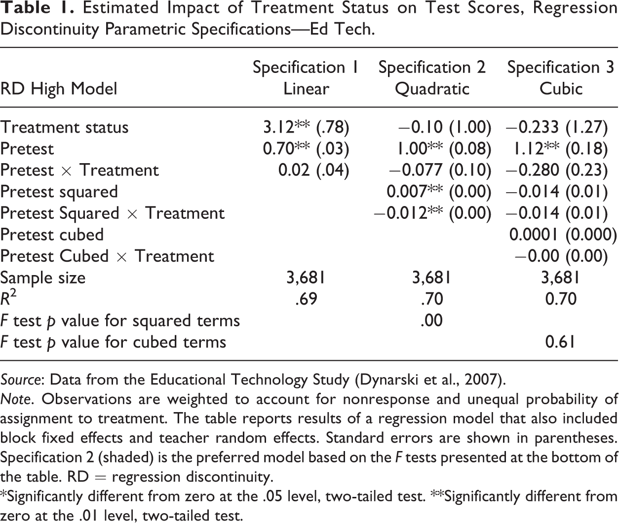
Table 1 presents the estimated impacts of the Ed Tech intervention from the parametric RD models (based on results for the RD high sample), with the regression results for the linear parametric specification in the first column, the quadratic specification in the second column, and the cubic specification in the third column. The p value for the F test for the joint significance of the squared terms was less than .005, indicating that these terms had predictive power in the model. By contrast, the p value for the cubic terms in the third column was .61, so we chose the quadratic model as our preferred specification. The estimated treatment effect in this specification was −.10 and not statistically significant. In other words, using a parametric RD model, we found that the ED Tech intervention did not significantly affect student test scores.

Table 1.

Estimated Impact of Treatment Status on Test Scores, Regression Discontinuity Parametric Specifications—Ed Tech.

RD High Model	Specification 1	Specification 2	Specification 3
RD High Model	Linear	Quadratic	Cubic
Treatment status	3.12** (.78)	−0.10 (1.00)	−0.233 (1.27)
Pretest	0.70** (.03)	1.00** (0.08)	1.12** (0.18)
Pretest × Treatment	0.02 (.04)	−0.077 (0.10)	−0.280 (0.23)
Pretest squared		0.007** (0.00)	−0.014 (0.01)
Pretest Squared × Treatment		−0.012** (0.00)	−0.014 (0.01)
Pretest cubed			0.0001 (0.000)
Pretest Cubed × Treatment			−0.00 (0.00)
Sample size	3,681	3,681	3,681
R ²	.69	.70	0.70
F test p value for squared terms		.00
F test p value for cubed terms			0.61

Source: Data from the Educational Technology Study (Dynarski et al., 2007).

Note. Observations are weighted to account for nonresponse and unequal probability of assignment to treatment. The table reports results of a regression model that also included block fixed effects and teacher random effects. Standard errors are shown in parentheses. Specification 2 (shaded) is the preferred model based on the F tests presented at the bottom of the table. RD = regression discontinuity.

*Significantly different from zero at the .05 level, two-tailed test. **Significantly different from zero at the .01 level, two-tailed test.

If we had used the linear model, the incorrect parametric specification, we would have concluded that the impact was statistically significant and positive at 3.12 normal curve equivalent (NCE) points. This highlights the importance of using the appropriate functional form in a parametric RD specification. The cost in statistical power of adding nonlinear terms to the specification can be seen in the estimated standard errors of the impact. The estimated standard error is higher in the cubic specification (1.27) than in the quadratic specification (1.00), but the point estimate is similar in the two specifications. In addition, Gelman and Imbens (2014) argue against including cubic or higher order polynomial terms in RD regressions because doing so leads to greater instability in the resulting impact estimates.⁵

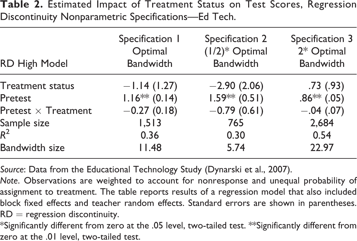
In the local linear (nonparametric) model, we used the algorithm described by Imbens and Kalyanaraman (2011) for selecting the optimal bandwidth. For the RD high Ed Tech sample, the optimal bandwidth was 11.48 points and Table 2 presents the nonparametric local linear impact estimates. Specification 1, using the optimal bandwidth (our preferred specification), yielded a point estimate of the Ed Tech impact of −1.14, which was not statistically significant. We also report results using bandwidths of one half and twice this optimal bandwidth as a sensitivity check. Under Specifications 2 and 3, using the alternate bandwidths, the estimated impact of the Ed Tech intervention was slightly different but also not significantly different from zero. The standard errors of these estimates were inversely related to the bandwidth size.

Table 2.

Estimated Impact of Treatment Status on Test Scores, Regression Discontinuity Nonparametric Specifications—Ed Tech.

RD High Model	Specification 1	Specification 2	Specification 3
RD High Model	Optimal Bandwidth	(1/2)* Optimal Bandwidth	2* Optimal Bandwidth
Treatment status	−1.14 (1.27)	−2.90 (2.06)	.73 (.93)
Pretest	1.16** (0.14)	1.59** (0.51)	.86** (.05)
Pretest × Treatment	−0.27 (0.18)	−0.79 (0.61)	−.04 (.07)
Sample size	1,513	765	2,684
R ²	0.36	0.30	0.54
Bandwidth size	11.48	5.74	22.97

Source: Data from the Educational Technology Study (Dynarski et al., 2007).

*Significantly different from zero at the .05 level, two-tailed test. **Significantly different from zero at the .01 level, two-tailed test.

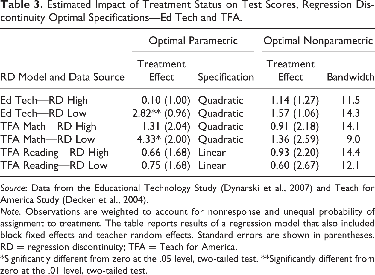
We repeated these procedures to select optimal parametric and nonparametric specifications for the Ed Tech RD low sample, the TFA math samples, and the TFA reading samples, and Table 3 summarizes these results.

Table 3.

Estimated Impact of Treatment Status on Test Scores, Regression Discontinuity Optimal Specifications—Ed Tech and TFA.

RD Model and Data Source	Optimal Parametric		Optimal Nonparametric
RD Model and Data Source	Treatment Effect	Specification	Treatment Effect	Bandwidth
Ed Tech—RD High	−0.10 (1.00)	Quadratic	−1.14 (1.27)	11.5
Ed Tech—RD Low	2.82** (0.96)	Quadratic	1.57 (1.06)	14.3
TFA Math—RD High	1.31 (2.04)	Quadratic	0.91 (2.18)	14.1
TFA Math—RD Low	4.33* (2.00)	Quadratic	1.36 (2.59)	9.0
TFA Reading—RD High	0.66 (1.68)	Linear	0.93 (2.20)	14.4
TFA Reading—RD Low	0.75 (1.68)	Linear	−0.60 (2.67)	12.1

Source: Data from the Educational Technology Study (Dynarski et al., 2007) and Teach for America Study (Decker et al., 2004).

Note. Observations are weighted to account for nonresponse and unequal probability of assignment to treatment. The table reports results of a regression model that also included block fixed effects and teacher random effects. Standard errors are shown in parentheses. RD = regression discontinuity; TFA = Teach for America.

*Significantly different from zero at the .05 level, two-tailed test. **Significantly different from zero at the .01 level, two-tailed test.

We conducted two sets of placebo tests that addressed threats to the validity of the RD design, for each sample. The first tested for discontinuities at the cutoff for baseline variables other than the pretest score. The second looked for spurious discontinuities in the relationship between the assignment variable and outcome at points other than the cutoff. The results supported the validity of the RD designs as implemented and are described in the Online Appendix Material.

Comparing the RD and Experimental Estimates

Our purpose in conducting the experimental analysis of Ed Tech and TFA data was to produce estimates of the impact of these interventions that could be used as the standard against which the RD impact estimates could be compared. As discussed above, we chose the local experimental estimate (the average impact among a restricted sample of students with pretest scores within a range of values around the median pretest score) as our benchmark estimate and also present a test of whether the ATE based on the full sample differs significantly from this local estimate. The “trimmed” sample included 45% of the overall Ed Tech student sample, 54% of the TFA math sample, and 55% of the TFA reading sample.

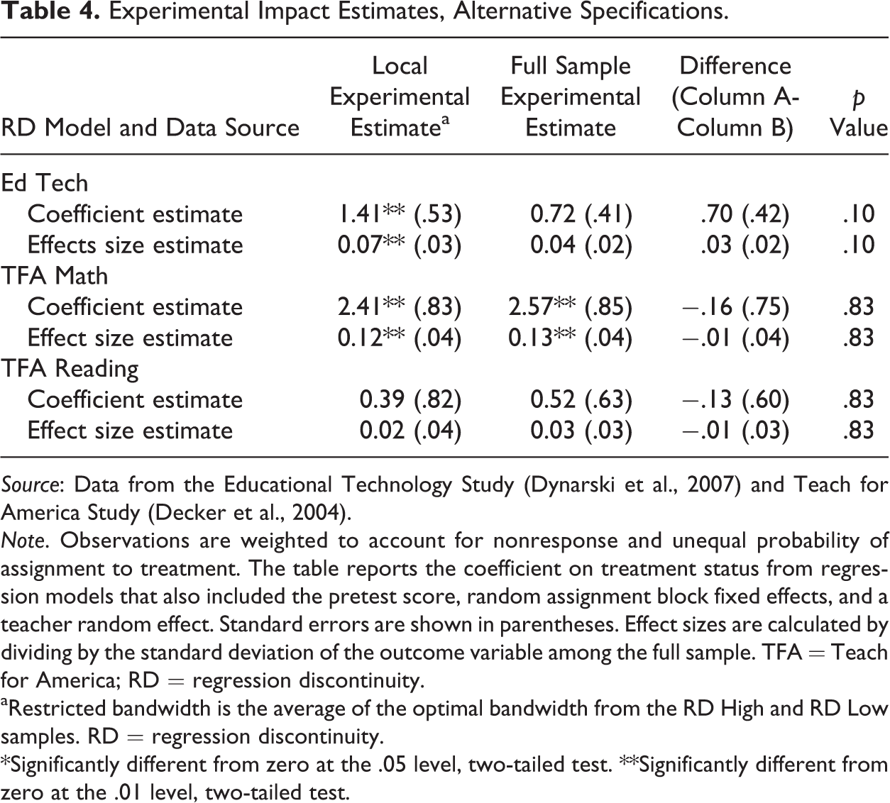
Table 4 shows the experimental impact estimates. For Ed Tech, the estimated local experimental impact was 1.41 points, which was statistically significant. This translates into an effect size of .07 standard deviation units. The $\hat{ATE}$ based on the full sample, shown in the second column of the table, was .72 points (an effect size of .04), and it is not statistically significant. It is worth noting that the local experimental estimate was significant and the $\hat{ATE}$ was not, and this highlights the importance of estimating the same causal estimand in WSCs (in this case, the local estimate). However, it is also the case that the difference between the local experimental estimate and the $\hat{ATE}$ was not statistically significant at the .05 level of statistical significance (p value = .10). For additional analysis of heterogeneity of treatment effects in these studies, see the Online Appendix Material.

Table 4.

Experimental Impact Estimates, Alternative Specifications.

RD Model and Data Source	Local Experimental Estimate^a	Full Sample Experimental Estimate	Difference (Column A- Column B)	p Value
Ed Tech
Coefficient estimate	1.41** (.53)	0.72 (.41)	.70 (.42)	.10
Effects size estimate	0.07** (.03)	0.04 (.02)	.03 (.02)	.10
TFA Math
Coefficient estimate	2.41** (.83)	2.57** (.85)	−.16 (.75)	.83
Effect size estimate	0.12** (.04)	0.13** (.04)	−.01 (.04)	.83
TFA Reading
Coefficient estimate	0.39 (.82)	0.52 (.63)	−.13 (.60)	.83
Effect size estimate	0.02 (.04)	0.03 (.03)	−.01 (.03)	.83

Source: Data from the Educational Technology Study (Dynarski et al., 2007) and Teach for America Study (Decker et al., 2004).

Note. Observations are weighted to account for nonresponse and unequal probability of assignment to treatment. The table reports the coefficient on treatment status from regression models that also included the pretest score, random assignment block fixed effects, and a teacher random effect. Standard errors are shown in parentheses. Effect sizes are calculated by dividing by the standard deviation of the outcome variable among the full sample. TFA = Teach for America; RD = regression discontinuity.

^aRestricted bandwidth is the average of the optimal bandwidth from the RD High and RD Low samples. RD = regression discontinuity.

*Significantly different from zero at the .05 level, two-tailed test. **Significantly different from zero at the .01 level, two-tailed test.

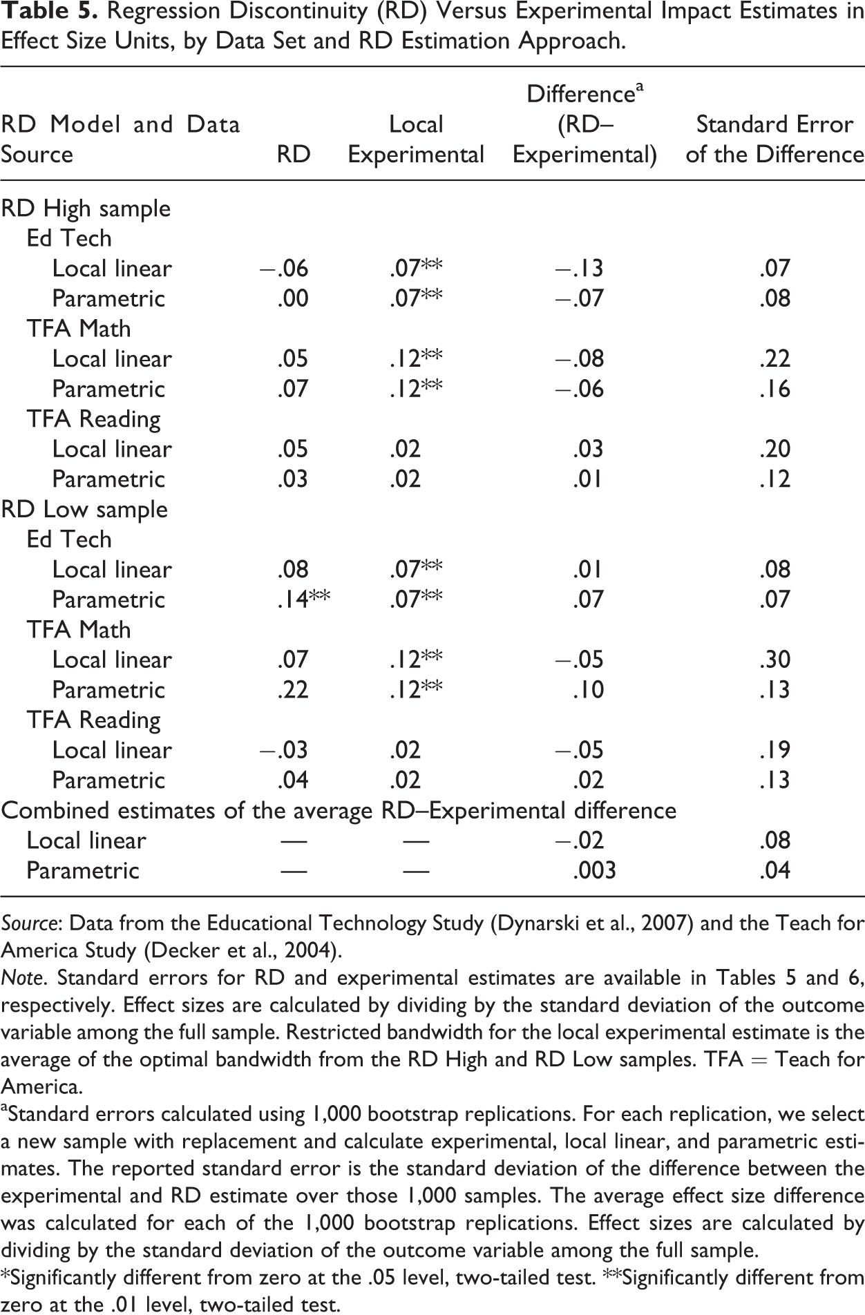
Table 5 shows the RD and experimental impact estimates of Ed Tech and TFA in effect size units, based on both the parametric and nonparametric (local linear) RD estimates. Estimates are shown for both the RD high and RD low samples. In each comparison, the RD and experimental impact estimates of these two educational interventions were not significantly different from one another. Across the 12 comparisons of RD versus experimental impact estimates in the RD high and RD low samples, there were no cases in which the difference was statistically significant at the .05 level.

Table 5.

Regression Discontinuity (RD) Versus Experimental Impact Estimates in Effect Size Units, by Data Set and RD Estimation Approach.

RD Model and Data Source	RD	Local Experimental	Difference^a (RD–Experimental)	Standard Error of the Difference
RD High sample
Ed Tech
Local linear	−.06	.07**	−.13	.07
Parametric	.00	.07**	−.07	.08
TFA Math
Local linear	.05	.12**	−.08	.22
Parametric	.07	.12**	−.06	.16
TFA Reading
Local linear	.05	.02	.03	.20
Parametric	.03	.02	.01	.12
RD Low sample
Ed Tech
Local linear	.08	.07**	.01	.08
Parametric	.14**	.07**	.07	.07
TFA Math
Local linear	.07	.12**	−.05	.30
Parametric	.22	.12**	.10	.13
TFA Reading
Local linear	−.03	.02	−.05	.19
Parametric	.04	.02	.02	.13
Combined estimates of the average RD–Experimental difference
Local linear	—	—	−.02	.08
Parametric	—	—	.003	.04

Source: Data from the Educational Technology Study (Dynarski et al., 2007) and the Teach for America Study (Decker et al., 2004).

Note. Standard errors for RD and experimental estimates are available in Tables 5 and 6, respectively. Effect sizes are calculated by dividing by the standard deviation of the outcome variable among the full sample. Restricted bandwidth for the local experimental estimate is the average of the optimal bandwidth from the RD High and RD Low samples. TFA = Teach for America.

^aStandard errors calculated using 1,000 bootstrap replications. For each replication, we select a new sample with replacement and calculate experimental, local linear, and parametric estimates. The reported standard error is the standard deviation of the difference between the experimental and RD estimate over those 1,000 samples. The average effect size difference was calculated for each of the 1,000 bootstrap replications. Effect sizes are calculated by dividing by the standard deviation of the outcome variable among the full sample.

*Significantly different from zero at the .05 level, two-tailed test. **Significantly different from zero at the .01 level, two-tailed test.

Based on other criteria for assessing the comparability of the RD and experimental impact estimates, the evidence is mixed. We first examined whether the RD and experimental estimates had the same general magnitude.⁶ In the 12 possible RD–experimental comparisons, the two estimates were within .05 effect size units of one another in 6 cases and between .06 and .10 effect size units in the remaining 6 cases. The RD and experimental estimates were the same sign in all but two cases. On the other hand, the statistical significance of the two sets of estimates frequently differed. The experimental impact estimate was statistically significant in 8 of the 12 cases, while the RD impact estimate was significant only once. For example, the experimental estimate of the impact of TFA on math achievement was .12 and statistically significant, while the local linear RD impact estimate was .07 and not statistically significant. In other words, a study based on this particular experimental design would have concluded that TFA had a positive impact on students’ math achievement, while a study based on this particular RD design (using a local linear specification) would not have found a statistically significant, positive impact of TFA on this outcome.

However, differences in statistical significance could arise either because of differences in the RD and experimental impact estimates themselves and/or because of differences in the statistical power of the two designs. In the designs used in this article, the power of the RD design was substantially lower than that of the experimental design both because of the correlation between the assignment variable and treatment status (Goldberger, 1972; Schochet, 2008) and because half of the experimental sample was dropped in creating the RD high and RD low analysis samples.

So while we found no significant differences between the RD and experimental estimates of the impacts of Ed Tech and TFA, other ways of assessing the comparability of the two sets of estimates suggest reason for concern. In particular, we would have needed to observe a large difference between the RD and experimental estimates to reject the null hypothesis that they were equal.

While the individual comparisons between a single RD estimate and single experimental estimate lacked statistical power, we could use the fact that we had many such comparisons. In the spirit of meta-analysis, we combined the results of six tests of the statistical significance of the difference between the RD and experimental impact estimates to summarize our evidence on the performance of the RD estimator. From the Ed Tech study, we used estimates based on both the RD high and RD low samples. From the TFA study, we used four sets of estimates: (1) the RD high sample for math, (2) the RD low sample for math, (3) the RD high sample for reading, and (4) the RD low sample for reading. Our overall estimate of the difference between an impact estimate based on an RD design versus one based on an experimental design was set to the mean value of the six individual difference estimates. The standard error of the overall difference was estimated using a bootstrap approach that accounted for any existing correlation between the estimates (such as correlation caused by the fact that for either the TFA RD high or RD low sample the same individuals were used in estimating the RD–experimental difference for math and reading). We conducted this analysis separately for the comparison of the local linear RD versus local experimental impact estimate and the comparison of the parametric RD versus local experimental impact estimate.

When we combined evidence from the six replication tests, we have stronger evidence regarding the estimated impact of a given intervention based on an RD design versus an experimental design. The average effect size difference between the RD and experimental estimates was less than .05 (bottom panel of Table 5). The average effect size difference for the parametric RD was .003, and the average effect size difference for the local linear RD was −.02. Neither of these estimated differences was statistically significant.

We can also examine these results to see whether the parametric or nonparametric specification performs better in this context. We find no clear advantage for one approach over the other. As indicated above, both the parametric and nonparametric RD specifications produced impacts that did not differ significantly from the experimental benchmark, on average. Looking at the individual comparisons in Table 5, the parametric estimate was closer in magnitude to the experimental benchmark in four cases and the nonparametric estimate was closer in two cases. In each of the six cases, however, there was no statistically significant difference between the parametric and nonparametric estimates. The parametric specification had a modest advantage in terms of statistical power, as the standard error of the RD–experimental difference estimate was smaller in the case of the parametric estimate. Overall, however, both the parametric and nonparametric produced impact estimates that matched those of an experimental benchmark. It is important to note, however, that the performance of parametric and nonparametric specifications could differ in other contexts, such as cases in which the functional form of the relationship between the assignment variable and outcome is different that it was here.

Manipulation of the Assignment Variable

In comparing the RD and experimental designs, we have implicitly assumed ideal implementation of the RD design. In other words, we assumed that all students whose true values of the assignment variable on one side of the cutoff were in the treatment group, while those whose true values were on the other side of the cutoff were in the control group. In practice, implementation of RD designs may not be perfect—there may be some manipulation of the assignment variable. This would occur when, for example, students whose true assignment variable values indicate they should be in the control group change those values to put them on the other side of the cutoff so they receive the intervention. School administrators or program operators may also be in a position to manipulate the assignment variable, to either ensure that particular students receive or do not receive the intervention.

When manipulation occurs, it has the potential to lead to bias in RD estimates of program impacts, but this bias would not be captured by the comparisons described above. Researchers facing this situation should assess this possibility in several different ways. Most importantly, they should learn as much as the can about how the underlying data were generated and assignment to the treatment group made in practice. For example, understanding the extent to which these processes were automated rather than involving conscious decisions by individuals may help researchers assess the likelihood of manipulation and its potential for bias. Once the data have been generated, the placebo tests described above (and in the Online Appendix Material) may be useful. For example, manipulation could cause discontinuities in the relationship between the assignment variable and other baseline variables at the cutoff, which would be a reason to question the validity of the design. Finally, manipulation may lead to discontinuities in the density of the assignment variable and the cutoff, so researchers should examine whether this is occurring.

In this section, we examine the extent of bias caused by various forms of manipulation and explore the diagnostic value of one specification test designed to detect the presence of manipulation (McCrary, 2008). The McCrary test examines the density of the assignment variable by smoothing out a histogram showing this density and looking for a jump, or discontinuity, at the cutoff value. It was the first formal test developed for the purpose of detecting manipulation and has been commonly used. More recently, other tests for detecting the presence of manipulation have been developed that relax some of the assumptions of the McCrary test and could be used as alternatives (Cattaneo, Jansson, & Ma, 2016; Otsu, Xu, & Matsuhita 2014). An important limitation of all of these tests is that they are not definitive. Some forms of manipulation will not be detected by tests focusing on the density of the assignment variable—for example, symmetric manipulation that involves values of the assignment variable being moved across the cutoff in both directions may not lead to a discontinuity in the density. However, these tests are useful in detecting some forms of manipulation.

We examine these issues using a series of simulations based on data files we create that simulate RD designs with the presence of manipulation of the assignment variable. In the simulations, we vary the extent of manipulation and the kinds of students whose assignment variable values are manipulated. By comparing impact estimates based on the data with and without such manipulation, we can estimate the resulting bias, defined as the difference between the impact estimate under the scenario with manipulation and the estimate under the scenario without manipulation. We also conduct the McCrary test to determine whether it detects manipulation under various scenarios.

Simulating the Presence of Manipulation

To simulate manipulation, we used the RD high data file in which students whose assignment variable is greater than the cutoff are in the treatment group and receive the intervention, while those whose assignment variable is less than the cutoff are in the control group and do not receive the intervention. We then made assumptions about the following aspects of the manipulation of the assignment variable:

Which direction is the cheating? We assumed that manipulation occurs in one direction only. In particular, we assumed that students whose true values of the assignment variable make them ineligible manipulate these values in order to be in the treatment group and receive the intervention.

What share of students cheat? We conducted different simulations that varied the fraction of ineligible students that manipulated the assignment variable (i.e., the fraction who “cheated” to receive the intervention), from 2% to 10% of all ineligible students in the sample.

Which students cheat? One might imagine that ineligible students who barely miss out on being eligible are more likely to “nudge” their assignment variable values just a little in order to become eligible. In other words, cheating might come entirely from students already close to the cutoff value. Alternatively, the likelihood that a student cheats may be unrelated to how close to the cutoff value they are. We simulate scenarios in which students who cheat are drawn from different ranges of values of the assignment variable.

Is the likelihood of cheating related to the outcome? A student’s propensity to cheat may be entirely unrelated to the outcome of interest in a study. Alternatively, it may be students whose unobserved characteristics are associated positively with the outcome who are most likely to cheat (or vice versa). For example, highly motivated students may be particularly likely to manipulate the assignment variable in order to receive the intervention. Conditional on the value of the assignment variable, we simulate both scenarios in which the likelihood of cheating is and is not related to the outcome.

To conduct a given simulation, we followed a four step process to determine which students cheated and to determine an outcome value for them under the assumption that they received the intervention. This process is described in Online Appendix Material.

In the end, we ended up with a simulated data set that included some cheaters. These students look just like students from the original RD high control group, except that their assignment variable is artificially high and they received the intervention, and so were defined as treatment group members under this simulation.

Simulating Manipulation: Results

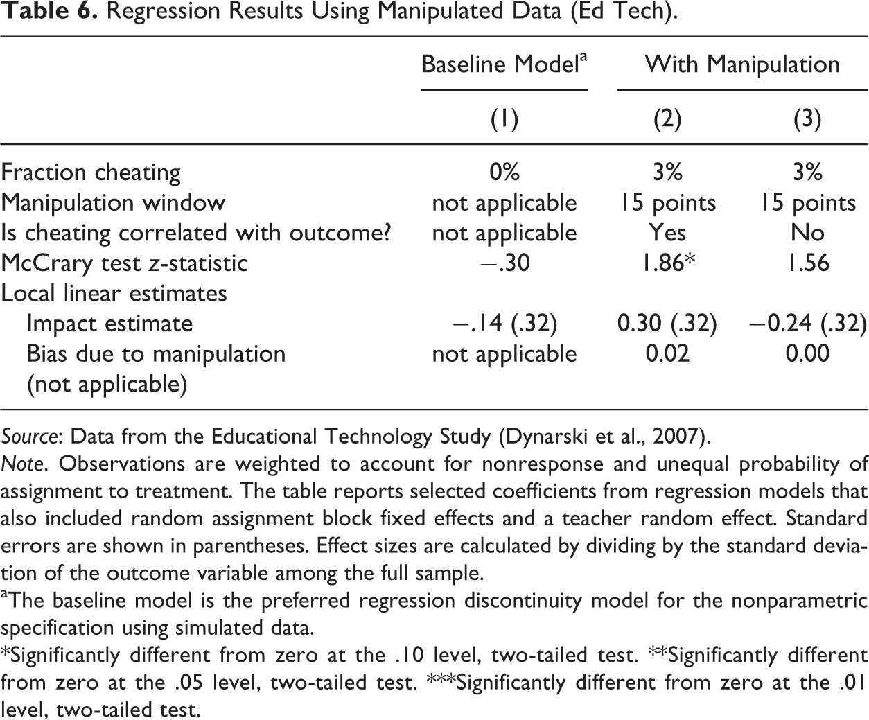
Table 6 shows the results of our manipulation simulations for two different manipulation scenarios. In each case, we assumed that 3% of the ineligible population cheats and that they are drawn from a window within 15 points of the cutoff (an area that includes about half of the overall RD high control group). In other words, those who manipulate the assignment variable are fairly close to the eligibility cutoff but not necessarily right on top of it. The 3% prevalence of cheating suggests that it is not rare, but neither is it rampant. The table shows results from two different simulations, one in which cheating is associated with the outcome and one in which it is not. Impact estimates from these simulations are compared with the original RD high baseline model, in which there is no manipulation of the assignment variable. For each scenario, the table also show the z-statistic from the McCrary test (McCrary, 2008) to detect manipulation. This is a test for a discontinuity in the density of the assignment variable. A statistically significant discontinuity would suggest manipulation, with some students changing their assignment variable values from one side of the cutoff to the other.

Table 6.

Regression Results Using Manipulated Data (Ed Tech).

	Baseline Model^a	With Manipulation
	(1)	(2)	(3)
Fraction cheating	0%	3%	3%
Manipulation window	not applicable	15 points	15 points
Is cheating correlated with outcome?	not applicable	Yes	No
McCrary test z-statistic	−.30	1.86*	1.56
Local linear estimates
Impact estimate	−.14 (.32)	0.30 (.32)	−0.24 (.32)
Bias due to manipulation (not applicable)	not applicable	0.02	0.00

Source : Data from the Educational Technology Study (Dynarski et al., 2007).

Note. Observations are weighted to account for nonresponse and unequal probability of assignment to treatment. The table reports selected coefficients from regression models that also included random assignment block fixed effects and a teacher random effect. Standard errors are shown in parentheses. Effect sizes are calculated by dividing by the standard deviation of the outcome variable among the full sample.

^aThe baseline model is the preferred regression discontinuity model for the nonparametric specification using simulated data.

*Significantly different from zero at the .10 level, two-tailed test. **Significantly different from zero at the .05 level, two-tailed test. ***Significantly different from zero at the .01 level, two-tailed test.

Column 1 presents estimates from the baseline (no manipulation) data set. The McCrary z-statistic of −0.30 is not statistically significant and hence provides no evidence of manipulation. This is not surprising given that there is no manipulation (by construction) in this case. The baseline RD impact estimate based on the nonparametric local linear specification is −.14, and not statistically significant.

Column 2 presents the results from the case in which there is manipulation that is correlated with the outcome. Figure 1 shows the density of the assignment variable in this case where each circle represents the density of observations within a given range of values of the assignment variable and the dotted line represents the local polynomial approximation of the density on either side of the cutoff. The figure shows what appears to be a modest discontinuity in this density, with the dotted line intersecting the cutoff from above at a higher level than from below. The z-statistic from the McCrary test is 1.86, which is marginally significant. The impact estimate in the presence of this form of manipulation is .30 (and not statistically significant), compared with −.14 (and not significant) in the baseline model. In other words, the estimated bias is .44 NCE points, which is equivalent to a modest effect size of .02. In this case, with the presence of a modest amount of manipulation that results in a modest bias, the McCrary test successfully detected the manipulation, though only if the researcher set the p value threshold for the presence of manipulation above .05.

Figure 1.

Density of pretest scores in manipulated data set (Ed Tech) with 3% cheating, 15 point window, cheating is correlated with outcome. Estimate of discontinuity at cutoff = 0.09. McCrary Test z-statistic = 1.86*. Source: Data from the Educational Technology Study (Dynarski et al., 2007). Each circle represents the density (shown on the y-axis) of observations falling within that cell of the assignment variable (shown on the x-axis). The dashed lines are local polynomial approximations of the density on each side of the cutoff.

In the case in which manipulation is not related to the outcome (column 3), the McCrary z-statistic is 1.56 and thus not significant. The impact estimate is −.24, close to the baseline impact estimate of −.14. In effect size units, the estimated bias is −.01.

Across other manipulation scenarios, a consistent set of results emerged when manipulation was assumed to be uncorrelated with the outcome (results available from authors). Under these scenarios, the result of the McCrary test was similar to the result with the same prevalence of manipulation drawn from the same manipulation window but where it was correlated with the outcome. However, regardless of the prevalence or manipulation window, estimated bias was close to zero under these scenarios. When manipulation is unrelated to the outcome measure, in other words, it does not lead to bias. However, the performance of the McCrary test is not related to whether or not manipulation is correlated with the outcome, which is not surprising given that this test is based on data from the distribution of assignment variable (in this case, pretest) values and does not depend on outcome values.

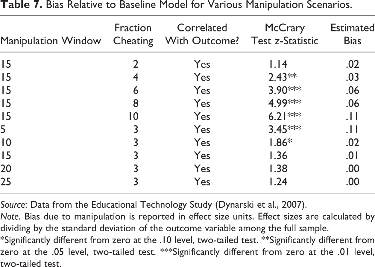
Hereafter, we discuss the results under scenarios in which manipulation is correlated with the outcome, which is the form of manipulation of greatest concern to researchers. Table 7 shows estimates of the McCrary z-statistic and bias under these scenarios. The top panel shows scenarios that vary according to the prevalence of cheating, with 2–10% of ineligible students assumed to have cheated. In each of these cases, we continue to assume that those who cheat have values of the assignment variable within 15 points of the cutoff. In the bottom panel, we assume that 3% of ineligible students cheat but vary the window from which those who cheat are drawn, from the area within 5 points of the cutoff to a larger area (45 points) that includes nearly all ineligible students.

Table 7.

Bias Relative to Baseline Model for Various Manipulation Scenarios.

Manipulation Window	Fraction Cheating	Correlated With Outcome?	McCrary Test z-Statistic	Estimated Bias
15	2	Yes	1.14	.02
15	4	Yes	2.43**	.03
15	6	Yes	3.90***	.06
15	8	Yes	4.99***	.06
15	10	Yes	6.21***	.11
5	3	Yes	3.45***	.11
10	3	Yes	1.86*	.02
15	3	Yes	1.36	.01
20	3	Yes	1.38	.00
25	3	Yes	1.24	.00

Source : Data from the Educational Technology Study (Dynarski et al., 2007).

Note. Bias due to manipulation is reported in effect size units. Effect sizes are calculated by dividing by the standard deviation of the outcome variable among the full sample.

The prevalence of cheating and the resulting level of bias is related to the ability of the McCrary test to detect cheating. When few students manipulate the assignment variable—for example, 2% of ineligible students drawn from within 15 points of the cutoff, the level of bias is low (equivalent to an effect size of .02) and the McCrary test does not detect a significant discontinuity in the density of the assignment variable. When manipulation is common—for example, 10% of ineligible students drown from the same 15 point window, there is substantial bias (equivalent to an effect size of .11) and the z-statistic from the McCrary test is clearly statistically significant.

Whether students who manipulate the assignment variable are those who just barely missed being eligible or come from throughout the range of ineligible students also is related to both the level of bias and the ability of the McCrary test to detect manipulation. When only those who just missed being eligible (within 5 points) manipulate the assignment variable, even when cheating is modest (3%), bias is substantial (0.11) and the McCrary z-statistic is significant. When the 3% who cheat come from a broader range of ineligible students, however, bias is low and the McCrary test is typically not significant.

Figure 2 shows bias and summarizes results of the McCrary test under a broader set of manipulation scenarios. Each point in the figure represents a given scenario, with the fraction cheating shown on the y-axis and the manipulation window shown on the x-axis. The estimated level of bias is low (less than .05) when the point is represented by a diamond, medium (.05 to .15) when the point is represented by a circle, and high (more than .15) when the point is represented by an x. The figure shows that when the manipulation scenario leads to moderate or high bias (and sometime in cases of low bias) the McCrary test detects a significant discontinuity in the density of the assignment variable. In other words, a strength of the test is that it is most likely to detect manipulation of the assignment variable in those cases in which this manipulation is most likely to lead to substantial bias. However, Figure 7 also shows that when manipulation is present and detected by the McCrary test, this does not necessarily imply that there is substantial bias. In a number of cases where the test detects manipulation, this manipulation leads to low levels of bias.

Figure 2.

Summary of bias for various manipulation scenarios (Ed Tech)—local linear specification, cheating is correlated with outcome. Cheating is correlated with outcome—Posttest must be above median. Source : Data from the Educational Technology Study (Dynarski et al., 2007).

Summary of Results

In this study, we set out to examine RD designs, and whether they produced similar impact estimates as experimental designs in two different studies of education interventions. We examined data from the Ed Tech Study and the TFA Study. In each case, we generated experimental impact estimates based on the original experimental data and then used a subset of the original data chosen in such a way that it could have come from a well-implemented RD study of the same intervention. We then estimated impacts of each intervention using the RD approaches and compared these estimates to the experimental estimates. Through this comparison, we could assess the extent to which the RD design produced results similar to the gold-standard experimental results.

A key limitation to this synthetic WSC approach for assessing the performance of the RD design is that it artificially ensured that the design was well implemented. In other words, we could be certain that the design was based on a single, well-defined assignment variable, that assignment to the intervention depended solely (and perfectly) on whether the value of the assignment variable was above or below a clear cutoff value, and that there was no manipulation of values of the assignment variable by individuals for purposes of gaining access to the intervention. As a result, our RD–experimental comparisons only allow us to assess the success of specific aspects of the RD approach—most importantly, the success of this design (in the context of two experimental studies) in modeling the relationship between the assignment variable and outcome and using the estimated discontinuity in this relationship at the cutoff value of the assignment variable as an estimate of the program impact. For example, we could compare parametric and nonparametric RD specifications in their ability to match the experimental benchmark. To address another key aspect of RD designs—the possibility that program applicants or operators manipulate the assignment variable to ensure that certain students receive the treatment, we also used the original experimental data to simulate a variety of scenarios in which such manipulation occurred.

We found that the RD and experimental impact estimates were not statistically different from one another in any of the six main RD–experimental comparisons, regardless of whether the comparison was based on the parametric or local linear (nonparametric) RD specification. Among the 12 estimates of the RD–experimental difference, the values ranged from −.09 to +.10 in effect size or standard deviation units. The magnitudes of six of the estimates were positive, and the remaining six were negative.

These original comparisons did highlight one major issue, the limited statistical power of the RD impact estimates resulting in limited power of the RD–experimental comparison. While none of the estimates was significant, differences between the two approaches as large as .09 or .10 standard deviation units could be substantively important in practice. This issue motivated us to calculate in the spirit of meta-analysis the average RD–experimental difference across the six comparisons (separately for the parametric and local linear RD specifications). When we did so, we again found no statistically significant difference between the estimates. In addition, the magnitude of the RD–experimental difference was small in absolute terms—.02 effect size units in the case of the parametric RD model and −.03 effect size units in the case of the local linear RD model.

In our examination of manipulation of the assignment variable, we focused on the diagnostic value of a specification test for the presence of manipulation (McCrary, 2008). In cases in which manipulation led to substantial bias in RD impact estimates, the test for a discontinuity in the assignment variable density at the cutoff proved to be a useful way of detecting the presence of manipulation as it consistently detected a significant discontinuity in cases in which manipulation led to moderate or high levels of bias in the RD estimates.

Supplemental Material

Supplemental Material, Appendix - RD or Not RD: Using Experimental Studies to Assess the Performance of the Regression Discontinuity Approach

Supplemental Material, Appendix for RD or Not RD: Using Experimental Studies to Assess the Performance of the Regression Discontinuity Approach by Philip Gleason, Alexandra Resch, and Jillian Berk in Evaluation Review

Footnotes

Declaration of Conflicting Interests

The author(s) declared no potential conflicts of interest with respect to the research, authorship, and/or publication of this article.

Funding

The author(s) disclosed receipt of the following financial support for the research, authorship, and/or publication of this article: This article was supported by funds from the National Center for Education Evaluation and Regional Assistance, Institute of Education Sciences (IES), under contract ED-04-CO-0112/000.

Supplemental Material

Supplemental material for this article is available online.

Notes

References

Barker

L. E.

Luman

E. T.

McCauley

M. M.

Chu

S. Y.

(2002). Assessing equivalence: An alternative to the use of difference tests for measuring disparities in vaccination coverage. American Journal of Epidemiology, 156, 1056–1061.

Black

Galdo

Smith

J. A.

(2007). Evaluating the bias of the regression discontinuity design using experimental data. Working paper, January 2007.

Buddelmeyer

Skoufias

(2004). An evaluation of the performance of regression discontinuity design on PROGRESA (Vol. 827), Washington, DC: World Bank.

Cattaneo

M. D.

Jansson

(2018). “Manipulation testing based on density discontinuity.” The Stata Journal, 18, 234–261.

Chiang

(2009). How accountability pressure on failing schools affects student achievement. Journal of Public Economics, 93, 1045–1057.

Cook

T. D.

Shadish

W. R.

Wong

V. C.

(2008). Three conditions under which experiments and observational studies often produce comparable causal estimates: New findings from within-study comparisons. Journal of Policy Analysis and Management, 27, 724–750.

Crump

R. K.

Hotz

V. J.

Imbens

G. W.

Mitnik

O. A.

(2008). Nonparametric tests for treatment effect heterogeneity. The Review of Economics and Statistics, 90, 389–405.

Decker

P. T.

Mayer

D. P.

Glazerman

(2004). The effects of teach for America on students: Findings from a national evaluation. Princeton, NJ: Mathematica Policy Research.

Dynarski

Agodini

Heaviside

Novak

Carey

Campuzano

… Sussex

(2007). Effectiveness of reading and Mathematics Software products: Findings from the First Student Cohort. Washington, DC: Institute for Education Sciences, National Center for Education Evaluation and Regional Assistance, NCEE 2007–4005.

10.

Gelman

Imbens

. (8 2014). Why high-order polynomials should not be used in regression discontinuity designs (Unpublished paper). Columbia University [http://www.stat.columbia.edu/∼gelman/research/unpublished/regression_discontinuity_14aug02.pdf]

11.

Goldberger

A. S.

(1972). Selection bias in evaluating treatment effects: Some formal illustrations (Discussion paper no. 129-72). Madison: University of Wisconsin, Institute for Research on Poverty.

12.

Green

D. P.

Leong

T. Y.

Kern

H. L.

Gerber

A. S.

Larimer

C. W.

(2009). Testing the accuracy of regression discontinuity analysis using experimental benchmarks. Political Analysis, 17, 400–417.

13.

Hahn

Todd

Van Der Klaauw

(2001). Identification and estimation of treatment effects with a regression discontinuity design. Econometrica, 69, 201–209.

14.

Hill

C. J.

Bloom

H. S.

Black

A. R.

Lipsey

M. W.

(2007). Empirical benchmarks for interpreting effect sizes in research. MDRC Working Paper on Research Methodology. New York, NY: MDRC.

15.

Imbens

Kalyanaraman

(2011). Optimal bandwidth choice for the regression discontinuity estimator. The Review of Economics and Statistics. First published online November 24, 2011.

16.

Imbens

Lemieux

(2008). Regression discontinuity designs: A guide to practice. Journal of Econometrics, 142, 615–635.

17.

Jacob

Lefgren

(2009). The effect of grade retention on high school completion. American Economic Journal: Applied Economics, 1, 33–58.

18.

Ludwig

Miller

(2005). Does head start improve children’s life chances? Evidence from a regression discontinuity design (Working Paper, #11702). National Bureau of Economic Research.

19.

McCrary

(2008). Manipulation of the running variable in the regression discontinuity design: A density test. Journal of Econometrics, 142, 698–714.

20.

Moss

B. G.

Yeaton

W. H.

LIoyd

J. E.

(2014). Evaluating the effectiveness of developmental mathematics by embedding a randomized experiment within a regression discontinuity design. Educational Evaluation and Policy Analysis, 36, 170–185.

21.

Niu

S. X.

Tienda

(2010). The impact of the Texas top 10 percent law on college enrollment: A regression discontinuity approach. Journal of Policy Analysis and Management, 29, 84–110.

22.

Otsu

K.-L.

Matsushita

(2015). Empirical likelihood for regression discontinuity design. Journal of Econometrics, 186, 94–112.

23.

Rindskopf

Shadish

W. R.

Clark

M. H.

(2018). Using Bayesian correspondence criteria to compare results from a randomized experiment and a quasi-experiment allowing self-selection. Evaluation Review. doi: 10.1177/0193841X18789532

24.

Rogers

Howard

Vessey

(1993). Using significance tests to evaluate equivalence between two experimental groups. Psychological Bulletin, 113, 553–565.

25.

Schochet

(2008). Technical methods report: Statistical power for regression discontinuity designs in education evaluations. Washington, DC: Institute for Education Sciences, National Center for Education Evaluation and Regional Assistance, NCEE 2008–4026.

26.

Shadish

W. R.

Galindo

Wong

V. C.

Steiner

P. M.

Cook

T. D.

(2011). A randomized experiment comparing random and cutoff-based assignment. Psychological Methods, 16, 179–191.

27.

Spybrook

Raudenbush

(2009). An examination of the precision and technical accuracy of the first wave of group randomized trials funded by the institute of education sciences. Educational Evaluation and Policy Analysis, 31, 298–318.

28.

Steiner

P. M.

Wong

V. C

. (2018). Assessing correspondence between experimental and non-experimental estimates in within-study comparisons. Evaluation Review. doi: 10.1177/0193841X18773807

29.

Tang

Cook

T. D

. (2018). Statistical power for the comparative regression discontinuity design with a pretest no-treatment control function: Theory and evidence from the National Head Start Impact Study. Evaluation Review, 42, 71–110.

30.

Tang

Cook

T. D.

Kisbu-Sakarya

(2015). Reducing bias and increasing precision by adding either a pretest measure of the study outcome or a nonequivalent comparison group to the basic regression discontinuity design: An example from education. Paper presented at the 2015 Society for Research on Educational Effectiveness Annual Conference, Washington DC.

31.

Van Der Klaauw

(2002). Estimating the effect of financial aid offers on college enrollment: A regression-discontinuity approach. International Economic Review, 43, 1249–1287.

32.

Wing

Cook

T. D.

(2013). Strengthening the regression discontinuity design using additional design elements: A within-study comparison. Journal of Policy Analysis & Management, 32, 853–877.

33.

Wong

V. C.

Steiner

P. M.

(2018). Designs of empirical evaluations of non-experimental methods in field settings. Evaluation Review. doi: 10.1177/0193841X18778918

Supplementary Material

Please find the following supplemental material available below.

For Open Access articles published under a Creative Commons License, all supplemental material carries the same license as the article it is associated with.

For non-Open Access articles published, all supplemental material carries a non-exclusive license, and permission requests for re-use of supplemental material or any part of supplemental material shall be sent directly to the copyright owner as specified in the copyright notice associated with the article.

0.00 MB

0.22 MB