
Abstract
Keywords
Economic evaluations of health programs commonly employ quality-adjusted life years (QALYs) as the unit of analysis, where QALYs are defined as life years times the health state utility measured on a 0.00 to 1.00 (death, best health) scale. Utilities have been increasingly measured using a multiattribute utility (MAU) “instrument”: a set of questions and response categories (the descriptive system or classification) and a corresponding set of utility weights.
The economic evaluation literature is presently dominated by 3 multiattribute utility instruments (MAUIs), the EQ-5D-3L, Health Utilities Index (HUI) 3, and SF-6D. A review of 1663 studies between 2005 and 2010 found that these 3 instruments accounted for 63.0%, 9.9%, and 8.8% of the total, respectively. 1 Four other instruments in the review, the 15D, HUI 2, Assessment of Quality of Life (AQoL), and Quality of Well-Being (QWB), were used in 7.0%, 4.6%, 4.2%, and 2.5% of the studies, respectively. The 1663 studies cited included 392 head-to-head comparisons between instruments. These generally found a low level of agreement between the utilities predicted for an individual's health state. Authors have generally concluded that MAU instruments are “imprecisely related” 2 and are “not interchangeable,” 3 a finding that threatens the comparability of evaluations that employ different instruments.
One response to these findings is to supplement existing descriptive systems to compensate for low sensitivity in a particular area. 4 A second proposal is to routinely include both a “reference method” and at least one additional method to reduce the likelihood of bias in the reference method. 5 A third suggestion is to value the results from different instruments using a common criterion such as the score on a visual analog scale (VAS) 6 or the rank order of health states. 7 Finally, crosswalks or mapping functions between instruments may be used to increase their comparability by aligning the numerical scales and possibly reweighting items. Following this approach, the aim of this article is to present estimated mapping functions between the main MAU instruments. Results reported here may be applied to extant results to increase the comparability of measurement.
Crosswalks between disease-specific or nonutility instruments and MAU instruments are now common and have been reviewed by both Mortimer and Segal 8 and Brazier et al. 9 One register alone documents 95 mappings to the EQ-5D-3L, 20 to the SF-6D, and 8 to the HUI 2 or HUI 3. 10
Crosswalks between MAU instruments are less common (for examples, see Fryback et al., 2 Seymour et al., 3 and Rowen et al. 11 ). However, they have the potential to lessen the incommensurability of MAU instruments and to allow best-practice cost-utility analysis (CUA). Ideally, the evaluation of a service should employ the MAU instrument, which is most able to identify changes effected by the service. However, if the utility scale of the most sensitive instrument compresses numerical values of incremental utilities, then the outcome of an evaluation might appear less favorable than the outcome of the evaluation of an inferior service that uses an MAU instrument, which inflates incremental utilities. The problem is illustrated with the results of the Multi-Instrument Comparison (MIC) survey described below. From pairwise regression, incremental utilities varied by more than 90% between instruments. Differences could not be explained by instrument sensitivity and were primarily attributable to differences in the scales used to calibrate the instruments.
In the present study, data from the same MIC survey were used to estimate crosswalk functions from each of the 6 MAU instruments included in the survey to each of the remaining 5 instruments. This implies the construction of 30 crosswalk functions: 6 (“initial”) instruments to be transformed into each of the 5 other (“target”) instruments. The results permit the utilities evaluated with any of the 6 initial instruments to be rescaled to increase comparability with the results that would be obtained from any selected target instrument.
The database used for the project and the statistical methods employed are described in the second section. Diagnostic statistics and mapping functions are reported in the third section. The use and limitations of the results are discussed in the fourth section.
Methods
Data
A MIC survey was carried out in 6 countries: Australia, Canada, Germany, Norway, United Kingdom, and United States. An online survey was administered by a global company, CINT Pty Ltd (Surrey Hills, Australia), to members of its panel. Respondents were initially asked to indicate if they had a current diagnosis of one of the chronic diseases in the study and to rate their overall health on a VAS where 0.00 represented death and 100 represented “best possible health” (physical, mental, and social). Quotas were then used to obtain a demographically representative sample of the “healthy” population, defined by the absence of chronic disease and a score above 70 on the VAS. Quotas were also applied to obtain a target number of respondents in each of 7 chronic disease areas: arthritis, asthma, cancer, depression, diabetes, hearing loss, and heart disease. In the following text, respondents with a chronic disease and those defined as “healthy” are referred to as “patient” and “public” respondents, respectively.
Responses were subject to 7 edit procedures based on a comparison of duplicated or similar questions. In addition, results were removed when an individual's (recorded) completion time fell below 20 minutes, which was judged to be the minimum time in which the 230 questions could be adequately considered and answered. The stringency of the criteria reflected the need for high-quality data and the lack of direct control inherent in a web-based survey. Edit procedures, the questionnaire, and its administration are described in detail online in Richardson et al. 12
The MAU survey instruments included are the MAUI described in Table 1. Instruments vary significantly in size, content, and the methods used for their construction. The 5-level EQ-5D-5L used in the study was derived from the EQ-5D-3L by Rabin et al. 13 It defines 3125 states; the QWB, SF-6D, 15D, and AQoL-8D define 945, 18,000, 3.1 × 10¹⁰, and 2.4 × 10²³ health states, respectively. Average completion times reported by authors vary from 1 minute (EQ-5D-3L) to 5.5 minutes (AQoL-8D). EQ-5D-5L has 1 psychosocial item; the SF-6D, 3 items; and the 15D, 5 items. AQoL-8D has 5 psychosocial dimensions consisting of 25 items. Two of the instruments scoring formulas were derived econometrically (EQ-5D-3L, SF-6D); 3 used decision-analytic procedures (HUI 3, 15D, QWB) and 1 used a combination of these methods (AQoL-8D). EQ-5D-5L utilities were based on “crosswalks” from the EQ-5D-3L. 13 The resulting utilities range from a maximum of 1.00 to a minimum of −0.59 (EQ-5D-5L). 1
MAUI Included in the MIC Study a
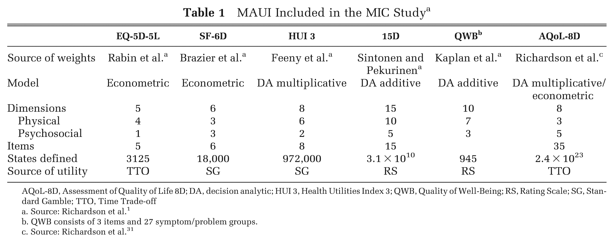
AQoL-8D, Assessment of Quality of Life 8D; DA, decision analytic; HUI 3, Health Utilities Index 3; QWB, Quality of Well-Being; RS, Rating Scale; SG, Standard Gamble; TTO, Time Trade-off
Source: Richardson et al. 1
QWB consists of 3 items and 27 symptom/problem groups.
Source: Richardson et al. 31
Econometrics Analysis
Mapping functions were derived from the regression of initial upon target instrument utilities. This requires a data set that includes individual responses to the relevant instruments. A mapping algorithm between them is then estimated using a flexible functional form and with an appropriate econometric technique. In the present study, a quadratic function was used to allow for a nonlinear relationship between instruments. Interaction terms were included between utility scores for each of the countries in the database. Sex was included as an explanatory variable. Other personal characteristics—age and education—were excluded because the comparability of the educational data between countries was not known and also because reliable and compatible data may not be collected by researchers using the present results. As age data are not always available to other researchers, the main results were estimated without age variables. However, the selected transformations were reestimated, including age dummies, and reported as supplementary material. The final functional form is given in equation (1).

The variable α is a constant. MAUi is the target MAUIi utility, MAUj is the initial MAUIi utility, ck is a set of country dummy variables, ckMAU is the interaction term between country variables and MAUj, Male is a dummy variable indicating the respondent is male, and i and j indicate the 6 MAU instruments (i≠j). The SF-6D is a reduced form of the SF-36. When the full SF-36 questionnaire has been administered, as commonly occurs in clinical trials, 8 validated dimension scores are available. AQoL-8D similarly subsumes 8 validated dimensions. For these two instruments, we further consider equation (2), in which 8 dimension values of SF-36/AQoL-8D are adopted as key predictors.

MAU_Dmj is the dimension m of the initial MAUj. Country dummies were included, but to simplify estimation procedures, the interaction terms were omitted.
Four econometric techniques were used to estimate the mapping algorithms. The first was the ordinary least squares (OLS) estimator, which has been the most widely adopted in the mapping literature.8,9 However, the assumption underlying OLS, that errors are normally distributed, is usually violated in mapping studies as data have an upper bound of 1.00. In addition, OLS is highly sensitive to outlier observations as it is based on the minimization of the variance of the residuals. The second technique, the censored least absolute deviations (CLAD) estimator, has gained popularity in recent years. It has 2 unique properties. First, it takes account of censoring of the dependent variable and, second, it achieves consistency if the error term condition on the independent variables has a median of 0. As such, the estimator is consistent even if errors are conditionally heteroskedastic (as usually occurs in mapping analyses). Since it is a median estimator, the CLAD estimator is robust to potential outliers.14,15 Despite these theoretical advantages, evidence suggests that mapping algorithms based on OLS often outperform CLAD.16,17
The third technique used in the study, the MM-estimator, is currently the most commonly used robust regression technique. 18 It builds on both an M-estimator (which minimizes some function of the residuals) and an S-estimator (which minimizes a measure of dispersion of the residuals) to achieve a high breakdown point with high efficiency. 19 To date, it has not been used in mapping exercises. The final technique was the generalized linear model (GLM), which allows for the nonnormal distribution of dependent variables such as the left/negatively skewed distribution of most utility scores. 20 GLM functions were estimated based on different distributions (Gaussian, binomial, and gamma) and with different functional forms (log and logit). The optimal combination of distribution and function was chosen for each mapping using the goodness-of-fit criteria described below. (Results are not reported but available from the corresponding author.) A stepwise regression technique was used to choose the “best” combination of predictors for OLS and GLM estimators. 21 The stepwise regression selected predictors based on the OLS estimator were considered for the CLAD and MM-estimators. Statistical significance was defined as P≤ 0.05.
If the measurement scale of the predicted and observed target utilities were perfectly aligned, then the regression of the predicted upon the observed utility would take the form Y = 0.00 + 1.00 *X, where X and Y are the predicted and observed utilities, respectively. This result necessarily occurs with OLS regression but not with the other estimators, implying a systematic bias in the predicted utilities. A second step adjustment was therefore used to rotate the first-stage estimates, X, derived from the non-OLS techniques, to align the scales of the predicted and observed utilities. To achieve this, the observed utility, Y, was regressed on the first-stage estimated utility, X, using OLS (equation (3)).

When a≠ 0.0 and b≠ 1.00, the measurement scales differ. To align the scales, a second-stage transformed utility, X*, was employed as defined by equation (4).

X* is the rotated value, derived from equation (3) by setting X* = Y. Consequently, it eliminates systematic bias caused by the technique. This may be seen by substituting X = X*/b – a/b (from equation (4)) in equation (3). The result is that Y = a+b[X*/b – a/b] = X*.
Validation and Goodness-of-Fit Measures
When no external database is available for the validation of an analysis, a common strategy in the mapping literature has been to randomly divide the original database into an estimation and a validation sample.21–24 Following this procedure, Stata's random-number generator (StataCorp LP, College Station, TX) was used to divide the MIC database into 2 mutually exclusive groups: an “estimation” and a “validation” sample containing 80% and 20% of the total sample, respectively. Both samples were created to retain the original proportion of respondents from each of the 6 countries.
Four goodness-of-fit measures calculated on the 20% validation sample were employed to evaluate results. The first was the difference between the predicted mean and observed mean utilities (ΔU). This criterion is advocated by Brazier et al. 9 as economic evaluation studies normally employ sample mean, rather than individual values, which suggests that selection criteria should be based on the correspondence of mean scores. The second criterion was the size of the intraclass correlation (ICC) between predicted and absolute utilities. This was preferred to the Pearson correlation, which may indicate a close linear relationship between variables despite large absolute differences (e.g., an individual's income and gross domestic product [GDP] may correlate highly through time despite large absolute differences). The ICC is an index of the agreement between the absolute magnitude of variables. It was calculated here using the 2-way mixed model as discussed by McGraw and Wong. 25 The final 2 criteria were the widely used mean absolute error (MAE) and root mean square (RMSE). The latter (RMSE) has been the most popular criterion in the mapping literature.24,26 However, Willmott and Matsuura 27 suggest that MAE is a superior criterion when measuring average model performance since it is a more natural measure of average error, and its interpretation is unambiguous. Another popular goodness-of-fit measure, R2, is not used as an evaluation criterion since this statistic is not available for all econometric methods. Nevertheless, corresponding R2 statistics from OLS estimates are reported in Supplemental Table S5. As there is no consensus on the choice of criteria, the regression was selected, which achieved the best result with respect to the majority of the 4 criteria. When the 4 were indistinguishable, OLS was selected because of its simplicity. Except for the ICC, which was calculated in SPSS version 21.0 (SPSS, Inc., an IBM Company, Chicago, IL), all other analyses were conducted in Stata version 12.1 (StataCorp LP).
Results
Data
Data were obtained from 9665 individuals. Edit procedures described earlier resulted in the removal of 17% of the total. Table 2 presents the age, sex, and educational status of the remaining 8022 respondents. Because quotas were imposed, the proportion of respondents from each country is similar (Australia, 17.8%; United States, 18.2%; United Kingdom, 16.9%; Canada, 16.6%; Norway, 14.7%; and Germany, 15.8%). For the same reason, the age, sex, and educational profiles of respondents within each country are similar. The numbers recruited from the disease area varied from 772 for cancer to 943 for heart disease. The 1760 “public” respondents were obtained by combining country samples that closely matched the age-sex profile in each country. Except in Norway and Germany, where the QWB was not administered (reducing the response for the QWB to 5576), each of the 8022 respondents completed the 6 MAU instruments along with sociodemographic questions. There were negligible missing data as the online program did not permit respondents to proceed until questions were completed. This resulted in a final sample of 8022. Details of the sample administration and editing in each country are provided in country-specific reports. 28
Characteristics of the Multi-Instrument Comparison Sample (n = 8022) a
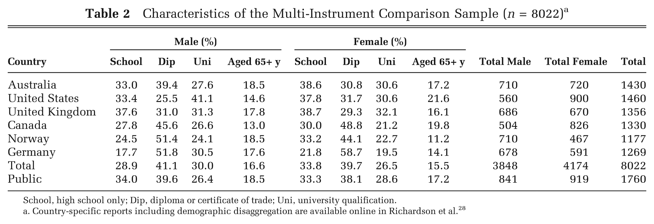
School, high school only; Dip, diploma or certificate of trade; Uni, university qualification.
Country-specific reports including demographic disaggregation are available online in Richardson et al. 28
Table 3 reports summary statistics for the 6 instruments. With the exception of the QWB and 15D, mean values are similar, varying from 0.83 to 0.88 in the public sample and from 0.68 to 0.74 in the full sample. Other characteristics of the sample differ more significantly. In the full sample, the standard deviation of the observations varies by 100% from 0.27 for HUI 3 to 0.13 for 15D and 0.14 for SF-6D. Ceiling effects (U = 1.00) vary from 19.1% (EQ-5D-5L) to 0.3% (AQoL-8D), and the percentage with a utility below 0.4 varies from 0.3% for the 15D and 1.3% for the SF-6D to 13.9% for HUI 3 and 14.7% for AQoL-8D. Differences in the distribution of utilities are illustrated in Figure 1. This plots the average utility predicted by each instrument for individuals in each percentile when individuals are ranked by the instrument's predicted utility. The figure indicates a nonlinear and varying relationship between instruments.
Summary Statistics of the Utility Scores for the 6 Multiattribute Utility Instruments
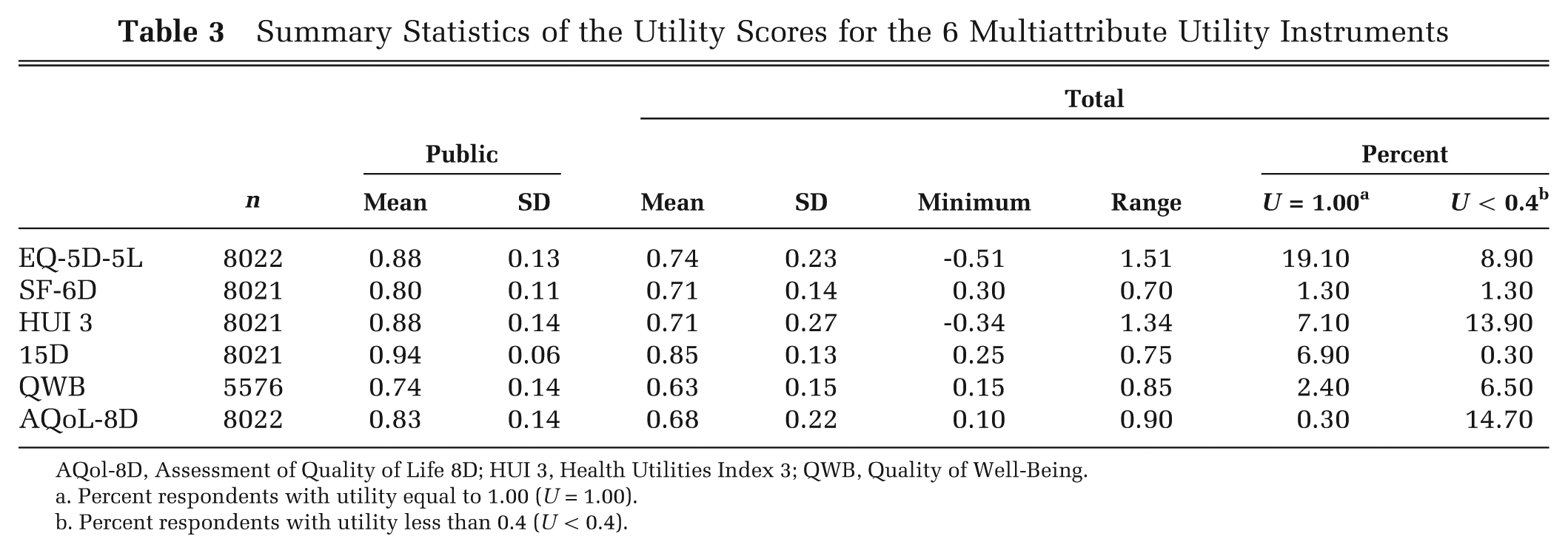
AQol-8D, Assessment of Quality of Life 8D; HUI 3, Health Utilities Index 3; QWB, Quality of Well-Being.
Percent respondents with utility equal to 1.00 (U = 1.00).
Percent respondents with utility less than 0.4 (U < 0.4).
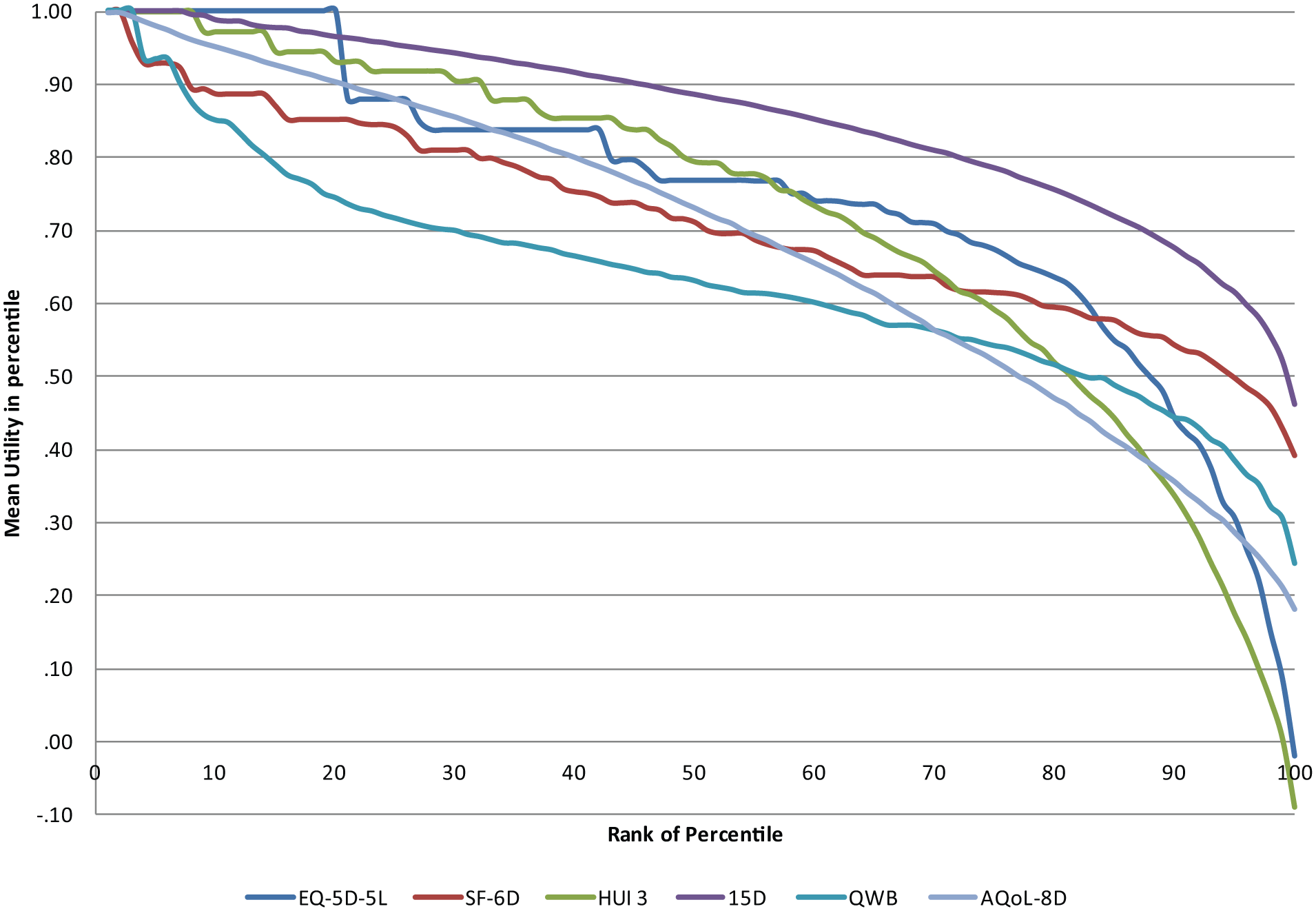
Mean utility per percentile by ranked percentile. AQol-8D, Assessment of Quality of Life 8D; HUI 3, Health Utilities Index 3; QWB, Quality of Well-Being.
Transformations
The main results are presented in 2 parts. First, the diagnostic statistics for all models are presented in Tables 4 and 5 (2 diagnostic statistics per table). Second, on the basis of these, the selected mapping functions (equation (1)) are reported in subsequent Tables 6 to 8. Transformations based on the dimensions of the SF-36 and AQoL-8D (equation (2)) resulted in better goodness-of-fit statistics. These transformations are reported in Supplemental Tables S1 and S2. Transformations including dummy variables for age are reported in Supplemental Tables S6 to S10.
Goodness-of-Fit: Difference in Average Utility and Intraclass Correlation Coefficients
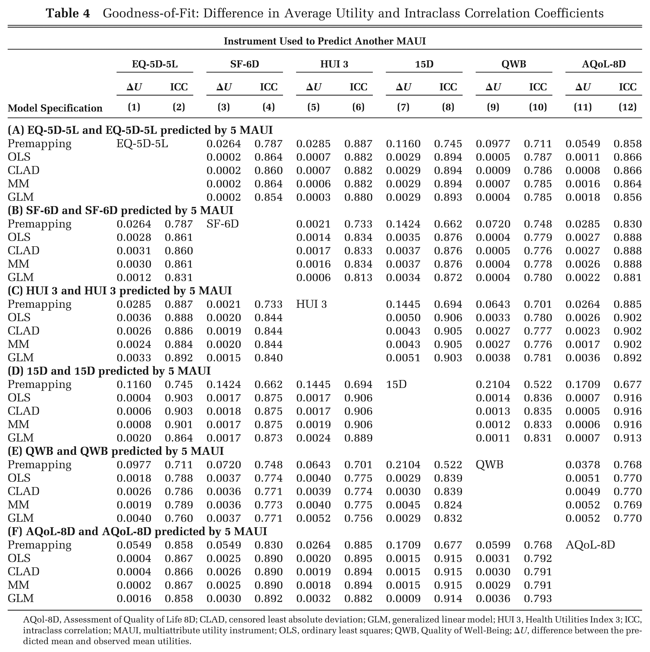
AQol-8D, Assessment of Quality of Life 8D; CLAD, censored least absolute deviation; GLM, generalized linear model; HUI 3, Health Utilities Index 3; ICC, intraclass correlation; MAUI, multiattribute utility instrument; OLS, ordinary least squares; QWB, Quality of Well-Being; ΔU, difference between the predicted mean and observed mean utilities.
Goodness-of-Fit: MAE and RMSE
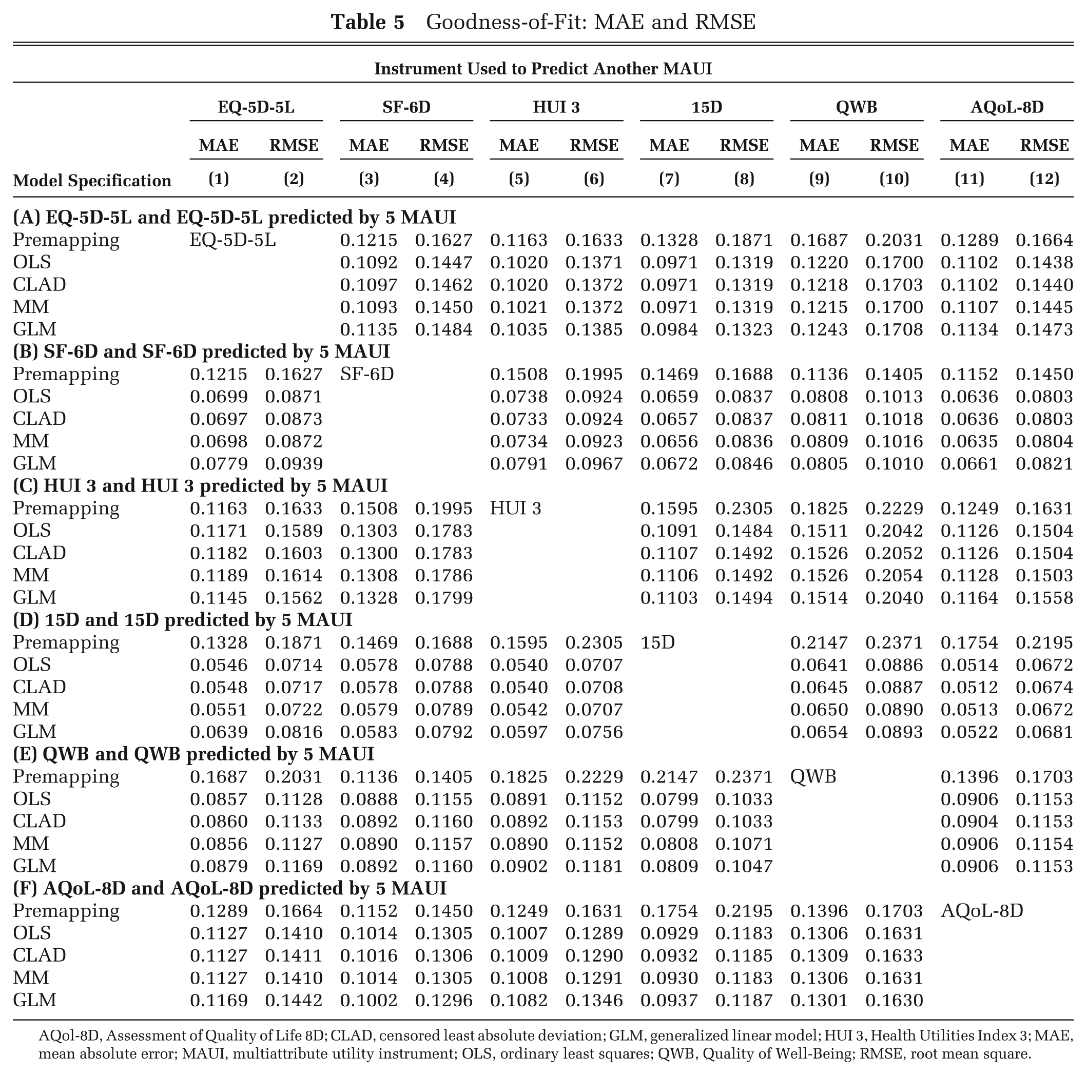
AQol-8D, Assessment of Quality of Life 8D; CLAD, censored least absolute deviation; GLM, generalized linear model; HUI 3, Health Utilities Index 3; MAE, mean absolute error; MAUI, multiattribute utility instrument; OLS, ordinary least squares; QWB, Quality of Well-Being; RMSE, root mean square.
Transformations: From EQ-5D-5L or HUI 3 to 5 Multiattribute Utility Instruments a
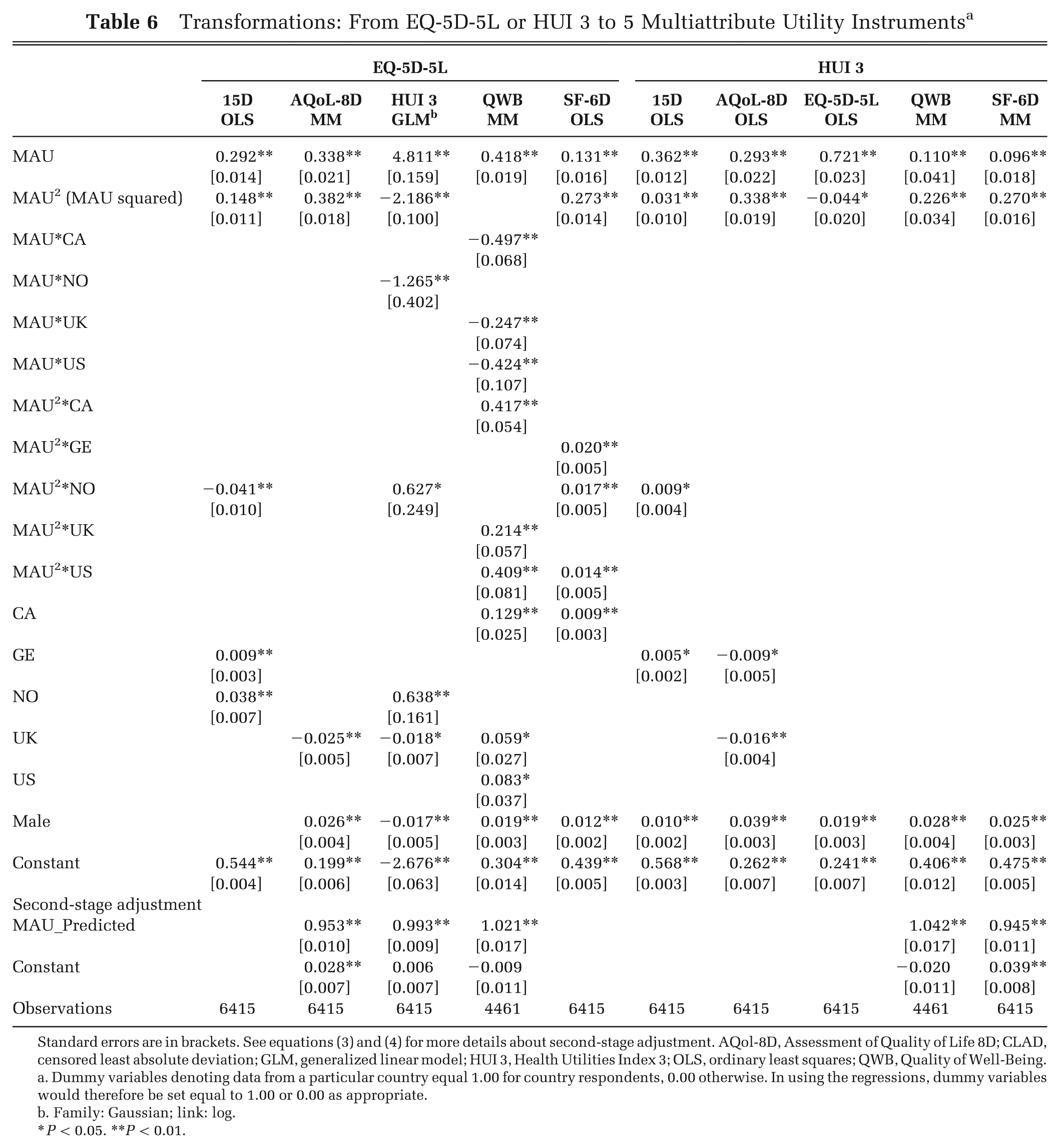
Standard errors are in brackets. See equations (3) and (4) for more details about second-stage adjustment. AQol-8D, Assessment of Quality of Life 8D; CLAD, censored least absolute deviation; GLM, generalized linear model; HUI 3, Health Utilities Index 3; OLS, ordinary least squares; QWB, Quality of Well-Being.
Dummy variables denoting data from a particular country equal 1.00 for country respondents, 0.00 otherwise. In using the regressions, dummy variables would therefore be set equal to 1.00 or 0.00 as appropriate.
Family: Gaussian; link: log.
P < 0.05. **P < 0.01.
Transformations: From 15D or QWB to 5 Multiattribute Utility Instruments a
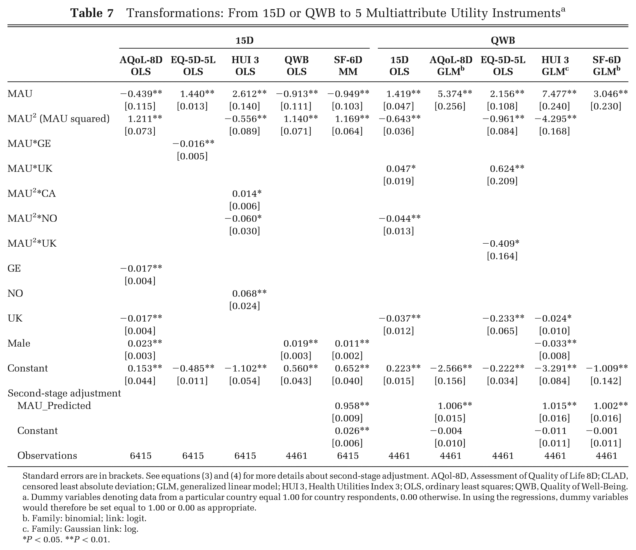
Standard errors are in brackets. See equations (3) and (4) for more details about second-stage adjustment. AQol-8D, Assessment of Quality of Life 8D; CLAD, censored least absolute deviation; GLM, generalized linear model; HUI 3, Health Utilities Index 3; OLS, ordinary least squares; QWB, Quality of Well-Being.
Dummy variables denoting data from a particular country equal 1.00 for country respondents, 0.00 otherwise. In using the regressions, dummy variables would therefore be set equal to 1.00 or 0.00 as appropriate.
Family: binomial; link: logit.
Family: Gaussian link: log.
P < 0.05. **P < 0.01.
Transformations: From SF-6D or AQoL-8D Utility to 5 Multiattribute Utility Instruments
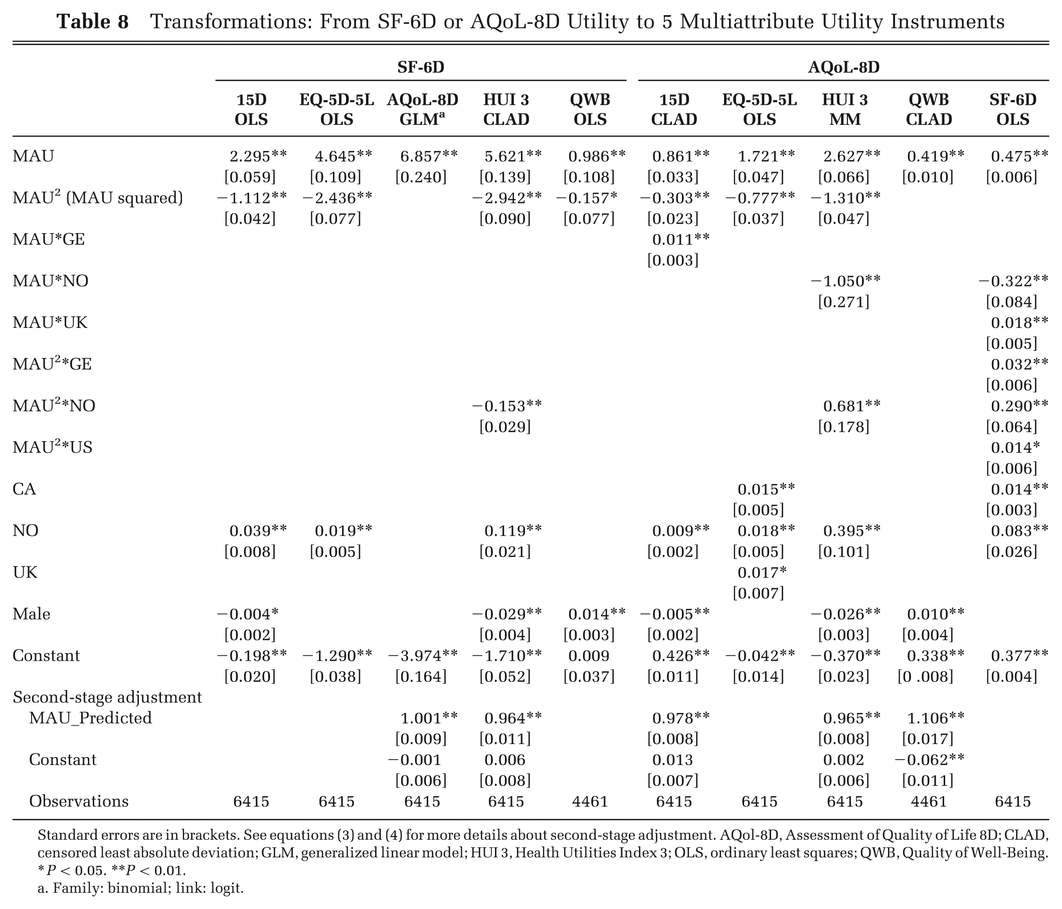
Standard errors are in brackets. See equations (3) and (4) for more details about second-stage adjustment. AQol-8D, Assessment of Quality of Life 8D; CLAD, censored least absolute deviation; GLM, generalized linear model; HUI 3, Health Utilities Index 3; OLS, ordinary least squares; QWB, Quality of Well-Being.
P < 0.05. **P < 0.01.
Family: binomial; link: logit.
From Table 4, the mean differences between target and transformed utilities are small and range from a minimum of 0.0002 (mapping from EQ-5D-5L to SF-6D using all estimators) to a maximum of 0.0052 (mapping from HUI 3 and AQoL-8D to QWB using GLM). All of the ICCs between the mapped and observed MAUI are above 0.756. The highest value, 0.916, is between the 15D and the 15D predicted from the AQoL-8D using OLS, GLM and MM estimators; the lowest, 0.756, is between QWB and QWB predicted by the HUI 3 using the GLM. Perversely, the ICC between the EQ-5D-5L and the EQ-5D-5L predicted from HUI 3 is lower, not higher, than the ICC between the instruments before the transformation. This may be due to the relatively poor prediction of negative EQ-5D-5L utilities and their better prediction by untransformed HUI 3 utilities, which also fall below zero.
From Table 5, transformations significantly reduced MAE, but the reduction was variable. Transformations to the 15D and SF-6D lowered the MAE by an average of 65% and 45%, respectively. Transformations to HUI 3 only reduced the MAE by an average of 18%. Instruments mapped into the 15D had the lowest MAE, and instruments mapped into HUI 3 had the highest. The RMSE gave consistent results but varied more than the MAE. The lowest coefficient (0.0512) was the mapping from AQoL-8D to 15D, and the highest (0.2054) was again from QWB to HUI 3. Overall, mapping to 15D again achieved the lowest RMSE and mapping to HUI 3 the highest.
The goodness-of-fit criteria that led to the selection of each of the functions (OLS, CLAD, MM, and GLM) are summarized in Supplemental Tables S3 and S4, and the corresponding regression results are presented in Tables 6 to 8. For non-OLS estimates, the second-stage adjustment is reported in the bottom block of the table, which reports the mapping. Only the final mapping equations are presented in this article. Other results are available from the corresponding author upon request.
Effects of the Transformations
The use of OLS regression or the application of the second-stage rotation of utilities resulted in transformed mean utilities, which were effectively identical to the means of the target instruments. (Means differ by 0.01 in only 2 cases.)
To test the effect of the transformation on the relative magnitudes of predicted change, pairwise OLS regressions were estimated of the form MAUi = a+b MAUj using the 20% sample. A coefficient of b = 1 indicates that, across the data set, the incremental change in utility—from one health state to another—predicted by the 2 instruments is, on average, equal. Deviation from b = 1 indicates the magnitude of the difference in quality-related QALYs, which would be obtained from the use of the 2 instruments. The b coefficients are summarized in Table 9. The differences pre- and posttransformation are generally very large. From the first column of Table 9, prior to transformation, incremental EQ-5D-5L utilities are 128% and 70% of the magnitude of incremental utilities estimated from SF-6D and HUI 3, respectively. After transformation of the latter 2 instruments, the incremental utilities differ by 4% and 3%, respectively. In 21 of the 30 posttransformation regressions, the discrepancy is 2% or less.
Ratio of Marginal Utilities: Pre- and Posttransformation (n = 1604)
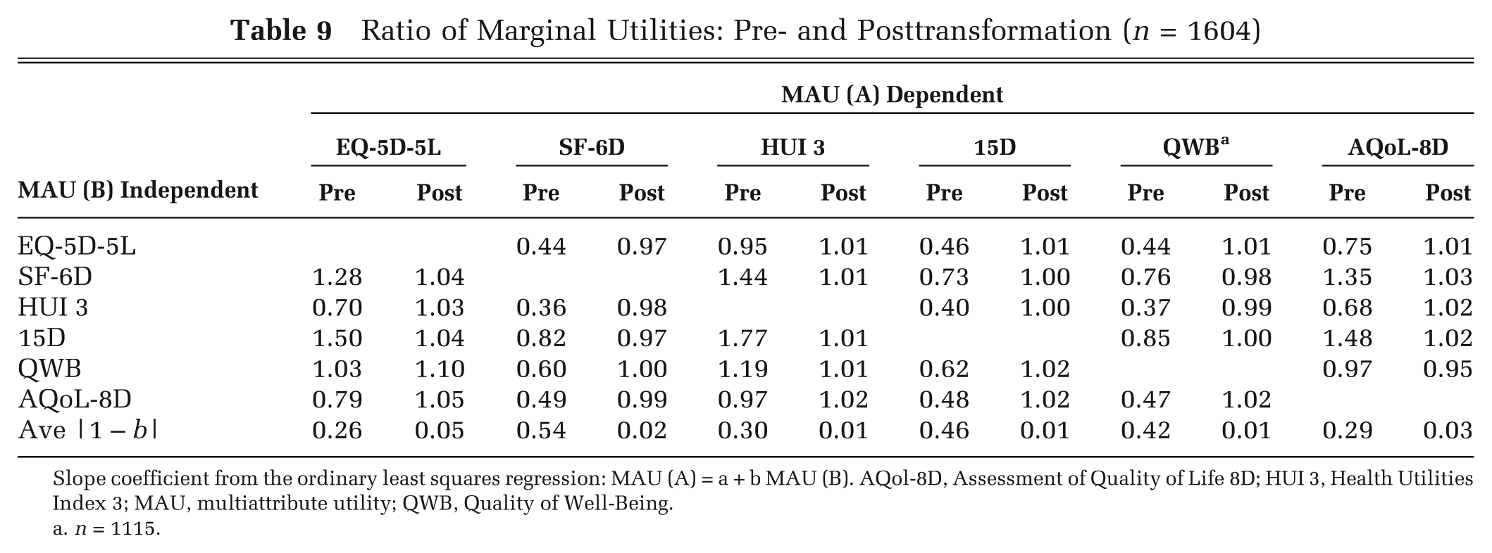
Slope coefficient from the ordinary least squares regression: MAU (A) = a + b MAU (B). AQol-8D, Assessment of Quality of Life 8D; HUI 3, Health Utilities Index 3; MAU, multiattribute utility; QWB, Quality of Well-Being.
n = 1115.
The addition of dummy variables for age, reported in the supplementary material, did not result in substantive change. The R2 from the regression of observed upon estimated data increased by an average of 0.008 (Suppl. Table S5).
Results from 6 of the 30 mappings are shown in Figure 2a–f. Figures for all other transformations are shown in the supplementary material. In each of the figures, individuals were ranked by the initial MAUI (i.e., by the instrument that was transformed). Individuals within each 2 percentile were grouped and the average initial, target, and transformed utilities plotted. The result is, by construction, a relatively linear plot for the initial utility and a relatively smooth plot for the utilities predicted from it. The average utilities for the target instrument result is a more erratic plot as it includes measurement error in both the initial and target instruments. This is most pronounced when the percentile of the initial instrument had few observations, either because of its scoring formula or, to the left of each figure, because the sample of extremely ill respondents was relatively small.
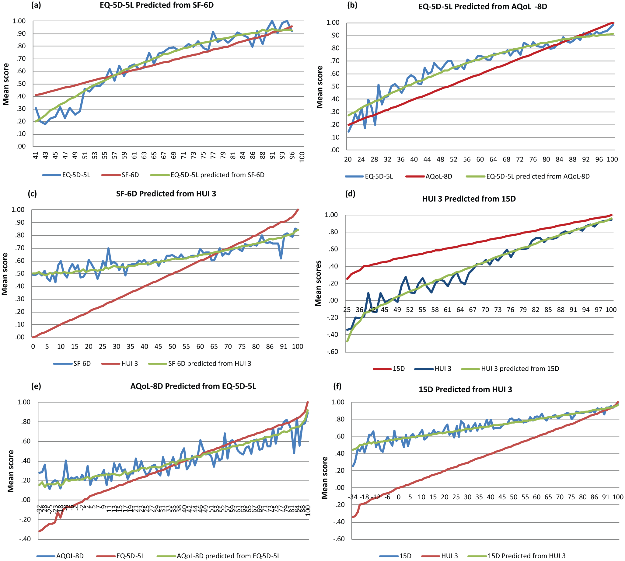
MAUi predicted by MAUj using the 20% sample. The range of utilities on the horizontal scale reflects the range of utilities predicted by the ranking instrument, further truncated at the bottom of the scale when there were 5 cases or less than per 2 percentile. AQol-8D, Assessment of Quality of Life 8D; HUI 3, Health Utilities Index 3.
Discussion
Utilities predicted by the 6 MAU instruments vary because of differences in their descriptive systems and in the methods adopted for generating utilities from the descriptive system. This has created an ongoing problem for CUA. The outcome of an economic evaluation may depend on the choice of instrument. The solution is not, as sometimes suggested, the use of a single instrument unless that instrument is the most sensitive available to every health state. The use of a single instrument implies a common standard, but the common standard may be biased. Analogously, the evaluation of every injury or illness with a psychosocial scale applies a common standard but one that would favor mental health programs and discriminate against most physical problems. Appropriate evaluation requires the use of appropriate instruments. In the context of CUA, this implies the use of the instruments that are most able to identify the changes associated with the services being evaluated.
However, this introduces a second problem as the different methods used to obtain utility scores from a health state description have imposed different scale properties that affect the numerical value of utilities in different ways. Transformations are one way of minimizing this second problem and help “level the playing field” in economic evaluation studies by allowing health states to be measured using the most sensitive instrument and then converting scores to a common “numeraire” scale. Alternative methods exist such as the valuation of instrument scores against an independent scale such as the Time Trade-off (TTO).6,7
By using a unique cross-country MIC data set, this study has generated 30 transformation equations between each of 6 MAU instruments. The goodness-of-fit results of the transformation equations are all within the range of previously published studies reported in the literature.9,17
This study has contributed to the methodological literature in this field in 2 ways. First, it has demonstrated the use of a robust MM-estimator that is able to take account of potential outliers in the data set. In several cases, the technique was found to produce superior results. However, the improvement was small, and despite its theoretical deficiencies, the classical OLS estimator was found to produce good results and was the preferred estimator in more than half of the transformations. Despite its claim to theoretical advantages, CLAD did not result in empirically superior results in any transformation.
The second contribution was the successful use of a second-stage adjustment when the OLS estimator was not used. The procedure increases the difficulty in estimating and interpreting the standard errors of the parameter estimates. Consequently, the benefit of the procedure was tested empirically by comparing goodness-of-fit statistics with and without the second-stage adjustment. Although not reported, we found that in most cases, the second-stage adjustment improved the goodness of fit. For example, the adjustment to the result of mapping HUI 3 into EQ-5D-5L using the MM-estimator was a significant reduction in the mean difference from 0.094 to 0.0005; a small reduction in the MAE and RMSE from 0.1031 to 0.1024 and 0.1390 to 0.1378, respectively; and an increase in the ICC from 0.874 to 0.882. The respective magnitudes of the improvements reflect the fact that the linear transformation of predicted scores would not be expected to significantly affect the MAE and RMSE, but the rotation of the estimates has a potentially large effect on absolute values and therefore the mean difference.
Transformations do not (and cannot) produce results that are identical to the utilities predicted by the target instrument. They cannot create content that is not in the initial instrument. Thus, for example, transformations from the EQ-5D-5L to the SF-6D cannot differentiate between the 19.1% of EQ-5D-5L respondents where U = 1.00 despite the SF-6D assigning U = 1.00 to only 1.3% of respondents (Table 2). Conversely, the majority of the transformations employed here cannot fully extinguish instrument content. With the exception of the dimension-based prediction from SF-36 and AQoL-8D, transformation functions are of the form MAU (target) = f[global MAU (initial)] (i.e., equation (1)). A change in a dimension of MAU (initial) that is excluded from MAU (target) will, nevertheless, alter global MAU (initial) and therefore alter MAU (target). With regression-based transformations, a dimension omitted from MAU (target) will nevertheless alter MAU (target) if the dimension is significant in the regression equation. However, a loss of content is possible in these transformations if a dimension is insignificant. From Supplemental Tables S1 and S2, the SF-36 dimensions RE and RB are not significant in several regressions, and the AQoL-8D dimensions of “relationships,”“happiness,”“senses,” and “self-worth” are insignificant in one or more results, implying a probable loss of some of the AQoL-8D psychosocial content in these regressions. However, the statistical insignificance of a dimension in a transformation function is a necessary but not sufficient condition for the extinction of content. It is possible that the content is transmitted through other dimensions, and it is for this reason that the dimension is insignificant. Consequently, separate analysis is needed to determine the extent to which content is diminished or extinguished in these cases. 28
The alignment of utilities has advantages and disadvantages. When the initial instrument measures the same content as the target instrument but with greater sensitivity, the transformation will allow the use of the more sensitive instrument while ensuring that the order of magnitude of the target and transformed utilities (and, more important, incremental utilities) are comparable. However, the alignment of utilities may result in bias when the descriptive systems of the instruments differ significantly. For example, for health states dominated by psychosocial problems, both the SF-6D and AQoL-8D may predict lower utilities than the EQ-5D-5L or HUI 3, which have fewer items measuring these dimensions. Transformation of the SF-6D or AQoL-8D into EQ-5D-5L utilities has the potential to reinflate the utilities and reduce (but not eliminate) the advantage these instruments have in measuring psychosocial health states. The extent to which this might occur has not been tested here.
While transformations permit utilities to be aligned with the scale embodied in a numeraire instrument, the choice of the numeraire may have a significant effect on the distribution of health resources between services that increase quality and those that increase the length of life. An MAU instrument whose scaling results in a wider range of utilities will, on average, favor services increasing quality of life (QoL). It will result in a larger numerical increase in estimated utility as QoL improves than an instrument that employs a narrower range. For example, from Table 3, a procedure that raised utility from the average of the full sample to the average of the healthy population would increase utility, measured by the EQ-5D-5L, by 0.14 (0.88–0.74) or by 18.9%. Measured by the SF-6D and the HUI 3, utility would increase by 12.6% and 23.9%, respectively. Use of the HUI 3 as the “numeraire instrument” would favor life improvement. Use of the SF-6D would favor life extension. The differences are not attributable to the sensitivity of the instruments—their ability to detect changes in health states—but to the numerical scale used to convert the changes into “utilities.” The choice of the numeraire instrument and the appropriate tradeoff between length and quality of life is a separate problem. The present study only seeks to minimize the random element attributable to the choice of instrument.
The study is limited in several respects. First, the use of a panel-based sample reduces quality control at the point of collection and recruits atypical respondents—namely, those who join a panel. Since the integrity of the present study depended on the reliability of results, the rigorous edit procedures described earlier were employed. As unsupervised panelists often minimize time answering questions, the removal of only 17% of respondents, despite 8 edit criteria, is probably attributable to the introductory letters from both the panel company and the research team, which emphasized the importance of the survey. The association found between instruments in the resulting database is greater than in comparable studies, suggesting that the procedure successfully removed unreliable respondents. 29 While panel members have atypical interests, the study required reliable, not representative, respondents. Selection from a large panel allowed the sampling of a very wide cross section of diseases and the inclusion of a significant number of respondents with poor health. (Table 3, for example, indicates that 8.9% and 13.9% of EQ-5D-5L and HUI 3 utilities were below 0.4.) This diversity of health states increases confidence in the validity of transformed results across a wide range of health states.
Second, the same algorithm was used to calculate the utilities for each of the 6 MAU instruments in each of the countries. In principle, each new set of weights requires the reestimation of the present function. The importance of this will vary with the discrepancy between the new weights and those used here, and, in practice, small differences may be accommodated by the adjustment of the new weights and the use of the reported functions. In principle, it would also be better to adopt country-specific algorithms to calculate the utilities for each instrument and for each country. However, most utility instruments do not have country-specific weights, and the weights used in the present study are commonly used in many countries. In empirical studies using cross-country data, the use of the same scoring algorithm for cross-country comparisons is not uncommon. 30
Third, to develop the mapping algorithms, 4 econometric methods were used. Alternatives exist that might be considered. Two-part models have gained popularity in mapping analyses because of their ability to handle problems arising from censored dependent variables (which may be particularly applicable for the EQ-5D-5L) (see Kay et al. 26 for an example). With the large sample size of the MIC data, the response mapping technique is a feasible alternative. Instead of predicting the utility directly, the response mapping approach first predicts the response levels of each item/dimension of the target instrument and, second, combines these using the target instrument's scoring algorithm to obtain utility scores. 8 These alternative approaches (potentially rescaled with alternative utility weights) may be tested by other researchers using the MIC data.
Conclusions
Crosswalks or transformations have been used primarily to obtain utility scores from disease-specific, nonutility instruments and thereby to allow a large volume of extant survey data to be used for economic analyses. However, transformations may also be used to increase the compatibility of results obtained from different MAU instruments. This, in turn, mitigates the problem arising from the uneven responsiveness of different instruments to different health states. Crosswalks between scales allow measurement with the most sensitive instrument and then the transformation of results to units defined by a selected “numeraire” instrument. Transformations do not produce identical scores: if they did, then the benefit of using a more sensitive instrument would be lost and the “numeraire” instrument should always be used. Rather, transformations align the scales of different instruments, which increases the comparability of results obtained from them.
The transformations described in this article allow the improved comparison of results obtained from 6 instruments. The algorithms for applying the transformations described here are available on the AQoL website (http://www.aqol.com.au/). The MIC data set is also freely available on the AQoL website for those who may wish to employ different methods or analyses to those reported here.
Footnotes
Financial support for this study was provided entirely by a grant from the National Health and Medical Research Council (NH&MRC) project grant (ID 1006334), “A Cross National Comparison of Eight Generic Quality of Life Instruments.” The German arm of the study was funded by Deutsches Krebsforschungszentrum (DKFZ) and the German Cancer Research Center in Heidelberg and conducted with the Institute for Innovation and Valuation in Health Care in Weisbaden. The Norwegian arm was facilitated by a grant from the University of Tromso.
References
Supplementary Material
Please find the following supplemental material available below.
For Open Access articles published under a Creative Commons License, all supplemental material carries the same license as the article it is associated with.
For non-Open Access articles published, all supplemental material carries a non-exclusive license, and permission requests for re-use of supplemental material or any part of supplemental material shall be sent directly to the copyright owner as specified in the copyright notice associated with the article.