Application of Mendelian Randomization to Investigate the Association of Body Mass Index with Health Care Costs

Abstract

Causal effect estimates for the association of obesity with health care costs can be biased by reversed causation and omitted variables. In this study, we use genetic variants as instrumental variables to overcome these limitations, a method that is often called Mendelian randomization (MR). We describe the assumptions, available methods, and potential pitfalls of using genetic information and how to address them. We estimate the effect of body mass index (BMI) on total health care costs using data from a German observational study and from published large-scale data. In a meta-analysis of several MR approaches, we find that models using genetic instruments identify additional annual costs of €280 for a 1-unit increase in BMI. This is more than 3 times higher than estimates from linear regression without instrumental variables (€75). We found little evidence of a nonlinear relationship between BMI and health care costs. Our results suggest that the use of genetic instruments can be a powerful tool for estimating causal effects in health economic evaluation that might be superior to other types of instruments where there is a strong association with a modifiable risk factor.

Keywords

bodymass index health care costs mendelian randomization obesity

Overweight and obesity are global public health concerns in terms of economic costs and effects on health.¹ The projected global prevalence of obesity will reach 18% in men and surpass 21% in women in 2025.² Higher body mass index (BMI), expressed in units of kg/m², is a risk factor for type 2 diabetes mellitus, cardiovascular diseases, and certain types of cancer, resulting in shortened life expectancy.³ According to the World Health Organization,⁴ individuals are classified as obese with a BMI $\geq 30$ kg/m². While lifestyle factors such as physical activity and nutrition are important drivers of obesity, there is also a significant genetic component: previous studies have suggested that at least 34% of BMI variation can be explained by genetic loci.^5,6

Accurate estimates of health care costs are crucial to judge the tradeoffs between medical possibilities, their financial viability, and quality and fairness in any health care system. Because of practical and ethical issues, many health risk conditions (e.g., obesity) cannot be assessed in randomized controlled trials (RCTs), and cost data collected in RCTs often have limited generalizability.⁷ On the other hand, observational studies can estimate the relation between health care costs and health conditions but generally cannot identify causal effects.⁸ Many previous studies that estimated the association of obesity with health care costs arise from observational studies (e.g., Finkelstein et al.,⁹ Trasande et al.¹⁰) that are unable to fully account for unmeasured confounders. For example, factors such as social deprivation or bias from self-reported height and weight measures are often not accounted for. In addition, the direction of the omitted variable bias is usually unclear. Cawley and Meyerhoefer⁸ discussed how some people became obese after suffering an injury or chronic depression and have higher medical costs because of the injury or depression. Carreras-Torres et al.¹¹ found that higher BMI increased the risk of being a smoker, but smoking itself lowers BMI.¹²

The presence of reverse causation and omitted variables motivated the use of instrumental variable (IV) analysis. The aim of the IV method is to exclude a correlation between the explanatory variables and the error term in a regression analysis. This is done by replacing the explanatory variables with other variables that are closely related to them but do not correlate with the error term.

For example, in the case of health care costs of obesity, Cawley and Meyerhoefer⁸ used the BMI of a biological relative as an IV. Compared with a standard ordinary least squares (OLS) model, the authors found a 4-fold increase in the marginal costs of obesity and a 3-fold increase in the marginal costs of 1 unit of BMI. Studies by Black et al.¹³ and Kinge and Morris¹⁴ found similar differences between OLS and IV models. They both used the BMI of a biological relative as an IV.

However, a potential concern with this approach is that unobserved characteristics may be correlated with both a person’s own BMI and his or her relative’s BMI, for example, when they live in the same household.¹⁵

In this article, we use an IV approach called Mendelian randomization (MR). MR is originally a concept from genetic epidemiology that uses genetic variants as IVs to overcome some limitations in cases where genetic polymorphisms have a well-known effect on modifiable risk factors such as BMI.¹⁶ If the IV assumptions hold, genetic variants can be used to estimate the effect of BMI on health care costs. Because genotypes are assigned randomly when passed from parents to offspring, the population genotype distribution is assumed to be unrelated to confounders and can therefore serve as a valid instrument. This random segregation of alleles, according to Mendel’s law of independent assortment, mimics a natural experiment in which individuals are randomly assigned to groups based on their exposure.¹⁷

Recent literature has suggested that MR can be a powerful tool for economic evaluation¹⁸; however, we only identified few studies that used it.^15,19–24

In this study, we use Mendelian randomization to estimate the effect of BMI on total annual health care costs and compare the results with a simple OLS model using data from a German population-based cohort study and published summary data.

Materials and Methods

Data

Study population

We use data from the KORA (Cooperative Health Research in the Augsburg Region) F4 study (2006–2010, $n = 3080$ ), a follow-up study of the S4 study (1999–2001, $n = 4261$ ) with a cross-sectional design. KORA is a population-based research platform in the region of Augsburg, a city in the south of Germany, and 2 surrounding districts running population-based epidemiological studies. A more detailed description of KORA can be found in Holle et al.²⁵ All KORA participants are German nationals and assumed to be of European ancestry (ethnicity is not recorded). Participants were interviewed at the study center regarding demographic and disease-related parameters, health care utilization, and medications. Weight and height measurements were performed by trained staff.

We also use summary-level data for individuals of European ancestry ( $n = 322, 154$ ) available from published genome-wide association studies (GWASs) by the Genetic Investigation of Anthropometric Traits (GIANT) consortium.²⁶

Confounders

All models adjust for age, sex, and education. Education was classified into 3 groups: basic education (≤ 9 years of schooling), medium education, and higher education (≥ 12 years of schooling, required to enter university). We also included the 10 first genetic principal components as covariates to control for residual population structure (allele frequency differences between cases and controls due to systematic ancestry differences) when estimating the BMI–health care costs summary-level effects from the KORA data.²⁷ Genetic associations should not be adjusted for large numbers of confounders, particularly if they may be on the causal pathway between the risk factor and the outcome.²⁸

Outcomes

The calculation of health care costs included outpatient services, hospital care, rehabilitation, and medication. Resource utilization of those services was assessed with an established questionnaire²⁹ and followed the standard way of how costs were calculated in previous KORA studies.³⁰ The time horizons for the assessment of used services varied from 7 days for medication, 3 months for outpatient physician contacts, and 12 months for inpatient and outpatient stays (hospital and rehabilitation). We extrapolated all measures to 12 months, under the assumption that the data were representative of the entire year, and then valued resource utilization by unit costs as provided by Bock et al.³¹ The costs of prescription medication were estimated using pharmacy retail prices, based on patient information on medication name and national drug codes. For details on the costing of resource utilization, please compare appendix Table A1. Table 1 presents an overview of the data set. Observations with missing (assumed at random) or implausible information were also removed, resulting in a sample size of $n = 2796$ (91% of whole sample).

Table 1

Summary Statistics for the KORA F4 Data Set^a

Characteristic	Overall
Annual total health care costs, mean (SD)	1961 (4325)
BMI, mean (SD)	27.7 (4.8)
Age, mean (SD)	56.2 (13.3)
Sex, n (%)
Female	1421 (50.7)
Male	1369 (49.3)
Education, n (%)
Basic	1451 (52)
Medium	681 (24)
Higher	664 (24)
Observations, n	2796

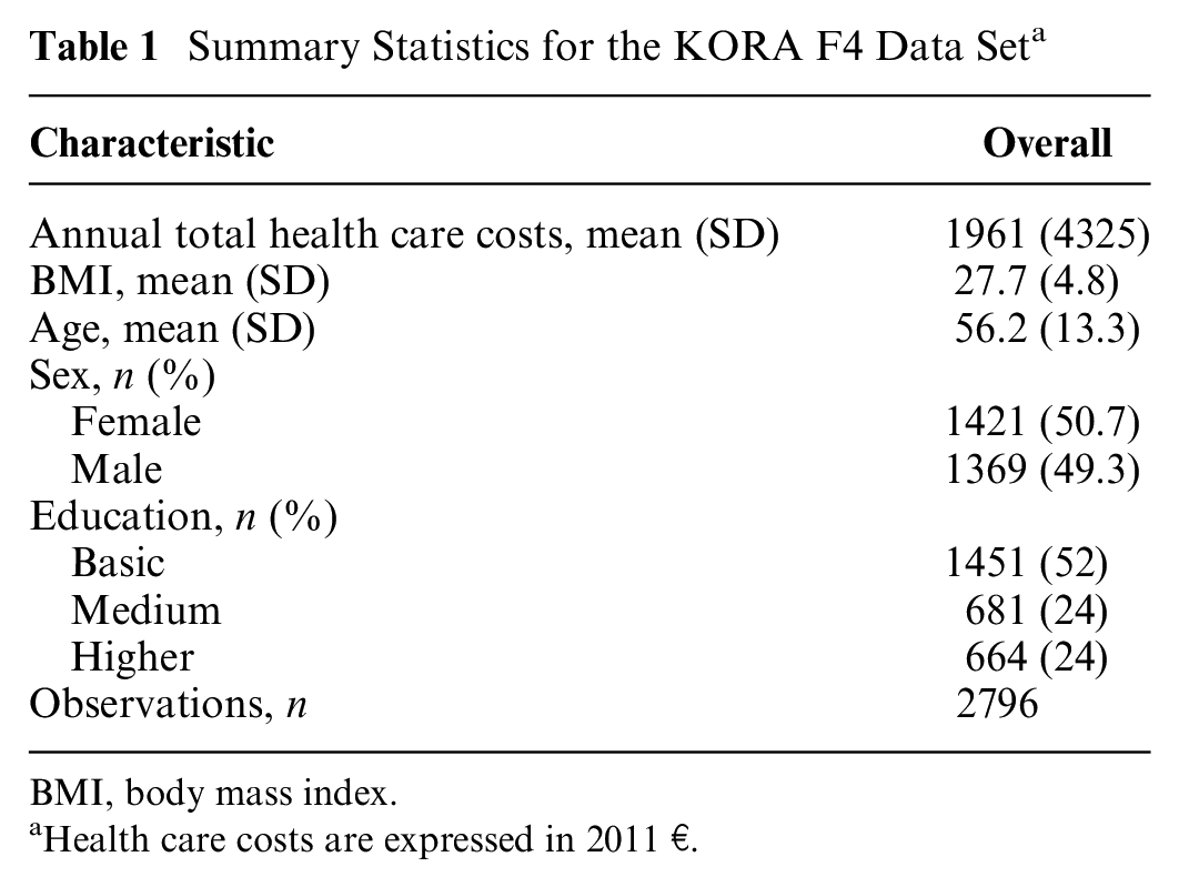
BMI, body mass index.

Health care costs are expressed in 2011 €.

Genetic instruments

We selected the 77 single-nucleotide polymorphisms (SNPs), out of the 97 reported (the remaining 20 SNPs are relevant for non-Europeans only), that are highly associated ( $P < 5 \times 10^{- 8}$ ) with BMI variation for individuals of European ancestry, based on a recent meta-analysis of 125 GWASs with 322,154 individuals by the GIANT consortium. A GWAS is a study of the genetic variation of the genome of an organism—designed to associate a particular phenotype (e.g., a disease) with particular alleles (a particular expression of a gene). The genes are not necessarily examined directly but well-defined markers such as SNPs. These are inherited and hereditary genetic variants. The SNPs reported in the GIANT study account for approximately 2.7% of BMI variation. (A newer study by Yengo et al.³² reports 716 SNPs that explain approximately 6% of the BMI variance, but these SNPs were not available to us.) The published estimates of the BMI–SNP association were based on an inverse normal transformation of BMI residuals on age, age², and any required study-specific covariates. Residuals were calculated by sex and case/control status in unrelated individuals and were sex adjusted among related individuals. We converted the causal estimates reported in standard deviations (SDs) to raw BMI units, assuming a median BMI SD of 4.6 kg/m².²⁶ Gene selection based on large consortia-based GWASs gives ideal candidates for MR studies.³³ All analyses were conducted in R³⁴ using the packages AER³⁵ and MendelianRandomization.³⁶

Mendelian Randomization

The IV method is used to estimate causal relationships when controlled experiments are not feasible or to infer causality in the presence of unmeasured confounding. An instrument is a variable that predicts the risk factor but, conditional on the risk factor, shows no independent association with the outcome. The random assignment in trials is an example of what would be an ideal instrument, but instruments can also be found in observational settings with a naturally varying phenomenon. For example, suppose a researcher wishes to estimate the causal effect of smoking on general health.³⁷ It is difficult to imply that smoking causes poor health because other variables, such as depression, can affect both health and smoking. An individual may start smoking because of depression, and simultaneously depression may influence health status. In addition, it is difficult to conduct controlled experiments on smoking status in the general population. In this case, the tax rate for tobacco products is a reasonable choice for an instrument for smoking, because higher prices tend to keep people from smoking. Moreover, tax rates for tobacco products are supposed to be unrelated to depression. If the researcher then finds an association between tobacco taxes and health status, this may be viewed as evidence that smoking causes changes in health.

Mendelian randomization is a type of IV analysis that uses genetic variants as instruments. The random allocation of genetic variants at conception means that these variants are less likely to violate some of the assumptions of IV analysis than nongenetic instruments, even describing it as nature’s randomized controlled trial.³⁸ A disease or trait does not alter the inherited alleles, and therefore these do not change over time. The SNP alleles’ random inheritance makes the genotype distribution largely independent of socioeconomic and lifestyle factors. Valid genetic instrumental variables are defined by 3 key assumptions (see Figure 1):

The genetic variant is associated with the risk factor of interest (the relevance assumption).

The genetic variant shares no common cause with the outcome (the independence assumption).

The genetic variants do not affect the outcome except through the risk factor (the exclusion restriction assumption).

Figure 1

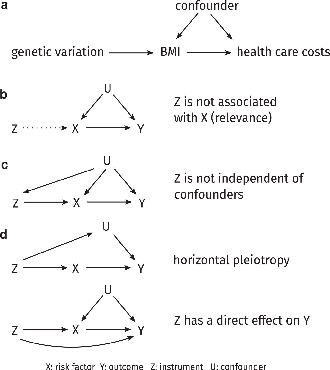
(a) A simplified causal diagram depicting our study. The instrumental variable (IV) assumptions are that the genetic variants are associated with risk factor body mass index (BMI), that they have no other influence on the outcome health care costs, except through BMI, and that there are no confounders of the genetic variants–outcome association. (b) An example of violation of the relevance condition: the instrument is not associated with the risk factor. (c) If, for example, variants associated with BMI had different frequencies in different ethnic groups, then the independence assumption would be violated. (d) The exclusion restriction assumption is violated in the presence of horizontal pleiotropy, in which genetic variants associated with the risk factor also affect a confounder. This assumption is also violated when the instrument has a direct effect on the outcome.

The first assumption is required because the risk factor will be estimated using the allele distribution of the genetic instruments. This assumption can be tested using the weak instruments test based on the first-stage F statistic.³⁹ The second and third assumptions are harder to validate because of potential pleiotropic effects of SNPs or SNPs in linkage disequilibrium (nonrandom association of alleles at different loci) correlated with genes that have effects on the outcome independently of the risk factor (see Figure 1c).⁴⁰ Another violation would happen if the sample consists of a population substructure with distinct distributions of alleles that is also linked with the outcome. In this situation, the substructure would be a prevalent cause of both SNP and outcome, opening up a path from SNP to nonexposure-mediated outcome (see Figure 1d). See Glymour et al.⁴¹ for examples violating the independence and exclusion restriction assumptions.

If the biological mechanism connecting the genetic variant to the risk factor is well understood, a single variant could plausibly fulfill these circumstances. In many cases, however, MR studies include multiple genetic variants. Then, for each of the genetic variants, the 3 main assumptions must hold.

In our study, we perform both one-sample MR using individual-level data and two-sample MR using summarized data. The one-sample analysis is based on the KORA data only, whereas the two-sample analysis uses the GIANT data for the SNP–BMI association and the KORA data for the SNP–health care costs association. We then meta-analyzed the MR estimates from each genetic instrument (SNP) from these analyses and report point estimates for the MR analyses together with standard errors (SEs) and 95% confidence intervals (CIs).

In the following, we explain both one-sample and two-sample approaches in more detail.

One-sample Mendelian randomization and 2-stage least squares

To estimate the impact of BMI on medical spending, we first used a 2-stage least squares (2SLS) model. In the first step of the 2SLS approach, the endogenous regressor of interest (BMI) is regressed on all valid instruments. As the instruments are assumed to be exogenous, this approximation of the endogenous variables will not correlate with the error term.

In the second step, the outcome (total annual health care costs) is regressed on the fitted values of BMI from the first stage.

Stage 1: Regress independent variable X (BMI) on instruments Z (genetic loci):

X = Z δ + ε .

(1)

Stage 2: Regress $Y$ (medical expenditures) on the predictions $\hat{X} = Z \hat{δ} = Z (Z^{T} Z)^{- 1} Z^{T} X$ from the first stage:

Y = \hat{X} β + η .

The 2SLS estimates are then

β_{2 SLS} = {(X^{T} Z {(Z^{T} Z)}^{- 1} Z^{T} X)}^{- 1} X^{T} Z (Z^{T} Z)^{- 1} Z^{T} Y .

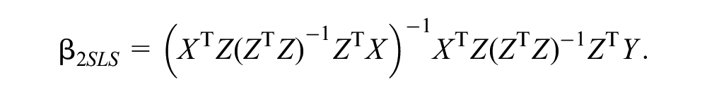
All 2SLS models control for age, sex, and education. This approach, using individual-level data in a single data set, is called one-sample MR. For comparison, we compute linear OLS non-IV models that regress health care costs on BMI and again adjust for the same covariates as before. We use the Durbin–Wu–Hausman endogeneity test⁴² to evaluate whether there is any evidence that the instrumental variable estimate differs from the OLS estimate. In this test, a significant result indicates disagreement between OLS and IV estimates.

Two-sample Mendelian randomization using summary data

Another popular MR method combines (publicly) available summary data on SNP–risk factor and SNP–outcome associations from 2 separate studies for large numbers of uncorrelated variants. These can be obtained from the published literature, typically from summary results provided by consortia of GWAS, or estimated directly from individual-level participant data. This is referred to as two-sample MR using summary data. The main advantage of two-sample MR is increased statistical power, but the quality of the pooled results is dependent on that of the individual studies. See Lawlor⁴³ for a detailed comparison of one-sample and two-sample MR.

Two-sample MR takes advantage of the fact that the risk factor–outcome association $β$ need not be known if instead the effect $γ$ of genetic variants $Z$ on outcome Y with error $κ$ is available:

Y = γ Z + κ .

Then the causal effect can be calculated using the Wald estimate⁴⁴:

β_{WALD} = \frac{\hat{δ}}{\hat{γ}},

where the estimate $\hat{δ}$ results from equation (1). It is important that both effect estimates $\hat{δ}$ and $\hat{γ}$ refer to the same alleles of the genetic instruments Z. Other than that, the same requirements apply as for 2SLS. As with MR in general, two-sample MR is analogous to methods originally developed in econometrics, and more information on the derivation of these estimators can be found in the literature.^45–47

In our study, we use the reported SNP–risk factor associations from the GIANT consortium and the SNP–outcome associations from the KORA data. Recently, a variety of different methods that go beyond the simple Wald estimate have been developed. We consider the 4 most common methods to calculate the causal effect of a two-sample MR study: the inverse variance weighted (IVW) method, the simple and weighted median, and MR Egger regression. The IVW meta-analysis of each Wald ratio is the easiest way to obtain an MR estimate using multiple SNPs. Using random effects allows each SNP to have different mean effects (e.g., due to horizontal pleiotropy), returning an unbiased estimate if the horizontal pleiotropy is balanced.

An alternative approach is to take the median effect of all available SNPs.⁴⁸ This has the advantage that only half the SNPs need to be valid instruments (i.e., robust association with the exposure, exhibiting no horizontal pleiotropy, no association with confounders) for unbiased estimation of causal effects. The weighted median can be obtained by weighting the contribution of each SNP by the inverse variance of its association with the outcome, so stronger SNPs contribute more to the estimate.

MR Egger regression⁴⁹ adapts the IVW linear regression analysis by allowing a nonzero intercept, so the net-horizontal pleiotropic effect (i.e., effects of the SNPs on the outcome not mediated by the exposure) across all SNPs can be unbalanced, or directional. The method returns an unbiased causal effect even if the horizontal pleiotropic effects are not correlated with the SNP–exposure effects (known as the InSIDE assumption). See Hemani et al.⁵⁰ for more details on all methods.

Invalid Instruments

As the number of biomarker-associated variants is constantly increasing through GWAS, selection of the most appropriate instruments is an important issue⁵¹ for one-sample MR. Using too many genetic variants as instruments can lead to spurious estimates and increased type I error rates. This implies that, even if a set of multiple instruments is valid (i.e., they are not associated with confounding factors, have no direct effect on the outcome, and are at least weakly associated with the exposure), the 2SLS estimator can still be biased toward the conventional regression estimate.^52,53 A weak instrument explains only a small proportion of the variation in the risk factor. Using many weak instruments can still result in weak instrument bias.^53,54 To address the weak instrument problem in the one-sample 2SLS models, we consider both least absolute shrinkage and selection operator (LASSO) variable selection and combining the genetic variants into a single risk score.

LASSO selection

LASSO selection suggests selecting optimal instruments in the first-stage regression by variable selection.⁵⁵ A similar approach with explicit application to MR was proposed by Kang et al.⁵⁶ Additional work by Windmeijer et al.⁵⁷ recommends using the adaptive LASSO to retain the oracle properties.⁵⁸ In the adaptive LASSO for the first stage, the goal is to minimize

min_{δ \in R^{p}} {\frac{1}{n} ‖ X - Z δ ‖_{2}^{2} + λ ∥ w δ ∥_{1}},

where $λ$ is a penalization parameter obtained by cross-validation, and $w = 1 / \hat{δ}$ is an initial estimate of $δ$ (e.g., obtained by least squares). The adaptive LASSO procedure that we used in our analysis shrinks many $δ$ parameters to effectively zero, pruning them out of the regression.

Genetic risk score

An individual’s genetic risk score (GRS) is equal to the number of alleles he or she has that are associated with an elevated risk factor; each person has zero, 1, or 2 alleles for each of the relevant SNPs, so a high score means a higher risk.²⁴ In our study, the 77 genetic variants from the Locke et al.²⁶ study result in a maximum possible GRS of 154.

The GRS has 2 benefits: first, it is stronger (explains more weight variation) than any of the SNPs separately, and second, it may be more valid as it decreases the likelihood that any alternative biological pathway (pleiotropy) in any single SNP will bias the IV outcomes.⁵⁹

However, Palmer et al.⁶⁰ showed that an unweighted score has lower power than adding multiple IVs into the 2SLS, and using an appropriately weighted allele score performs similarly to adding each valid SNP as an instrument.

Meta-analysis

We meta-analyzed the MR estimates from each genetic instrument (SNP) from the 6 individual analyses (one-sample 2SLS with GRS, one-sample 2SLS with LASSO, two-sample simple median, two-sample weighted median, two-sample IVW, two-sample MR Egger), assuming an inverse variance-weighted random-effects model to avoid overprecision and to allow for heterogeneity in the causal estimates.⁶¹

Pleiotropy

A common problem in MR analyses is the presence of pleiotropic effects (i.e., a genetic variant has associations with more than 1 risk factor on different causal pathways).⁶² This can be especially problematic for polygenic risk factors such as BMI, where the influence of genetic variants is less specific.⁶³ To test violations of the IV assumptions, we used 3 approaches. First, we checked, in the Phenoscanner database,⁶⁴ whether genes related to BMI are also significantly associated with other determinants of health care costs. In a second check, we used the MR Egger intercept test⁴⁹ for pleiotropy. In MR Egger regression, the intercept is left unconstrained to test for evidence of bias-generating pleiotropy, with a null hypothesis of no pleiotropic effects. As a third test for pleiotropy, we conducted Sargan’s test for overidentification.⁶⁵ This test is only available for one-sample MR with multiple instruments (i.e., the 2SLS analysis with LASSO selection). The null hypothesis in this test is that all exogenous instruments are in fact exogenous and uncorrelated with the model residuals, and all overidentifying restrictions are therefore valid.

Nonlinearity

Previous research found evidence of a nonlinear relationship between BMI and health care costs,^8,66 and MR is often unable to detect such nonlinearities because genetic variants usually explain only a small percentage of the variance in the risk factor.⁶⁷ We used the method of Staley and Burgess,⁶⁷ which assesses nonlinear exposure–outcome relationships using IV analysis in the context of MR. To test for nonlinear effects of BMI on health care costs in our sample, we fitted both a fractional polynomial model and a piecewise linear model and performed the Cochran Q test, quadratic test, and fractional polynomial test. The heterogeneity test using Cochran’s Q statistic is used to assess whether the localized average causal effect (LACE) estimates differ more than would be expected by chance. The second is a trend test where the LACE estimates are meta-regressed against the mean value of the exposure in each stratum, equivalent to fitting a quadratic exposure–outcome model. The third test is a more flexible variant that compares twice the difference in the log-likelihood between the linear model and the best-fitting fractional polynomial of degree 1 with a $χ_{1}^{2}$ distribution. Age, sex, and education are included as covariates in both models.

Results

One-Sample MR

Table 2 presents the results of the association between BMI and health care costs, according to the one-sample analysis. The OLS model finds an effect of €75.8 (SE 14.6) for a 1-unit increase in BMI. In contrast, the 2SLS model using the GRS estimates an effect of €129.0 (SE 241.2) for a 1-unit increase in BMI. The 2SLS LASSO model selects 64 valid genetic instruments for BMI and finds an effect of 146.1€ (SE 190.8). Other significant cost drivers or savers in the OLS models are age and higher education for the BMI model, but all associations lose significance at the 0.05 level when moving from OLS to 2SLS analysis.

Table 2

Effect of BMI on Annual Total Health Care Costs Using an OLS Model and Two One-Sample 2SLS Models with Genetic Variants as Instrumental Variables^a

Dependent Variable: Annual Total Health Care Costs	OLS	2SLS (GRS)	2SLS (LASSO)
Age	40.6^b	37.0^c	26.5
	(5.4)	(21.5)	(18.1)
Sex = female	211.3	241.2	219.3
	(136.3)	(308.1)	(340.4)
BMI	75.8^b	129.0	146.1
	(14.6)	(241.2)	(190.8)
Education
Basic	Reference	Reference	Reference
Medium	−35.2	34.3	328.8
	(170.5)	(436.8)	(474.1)
Higher	−426.8^d	−324.0	262.0
	(176.2)	(620.8)	(554.4)
Constant	−3026.8^b	−4381.3	−4042.3
	(544.0)	(7858.3)	(4949.3)
Observations	2796	2796	2796
Weak instruments test P value		0.01	0.04
First-stage F statistic		22.0	18.4
Durbin–Wu–Hausman test P value		0.86	0.64
Sargan test P value			0.99

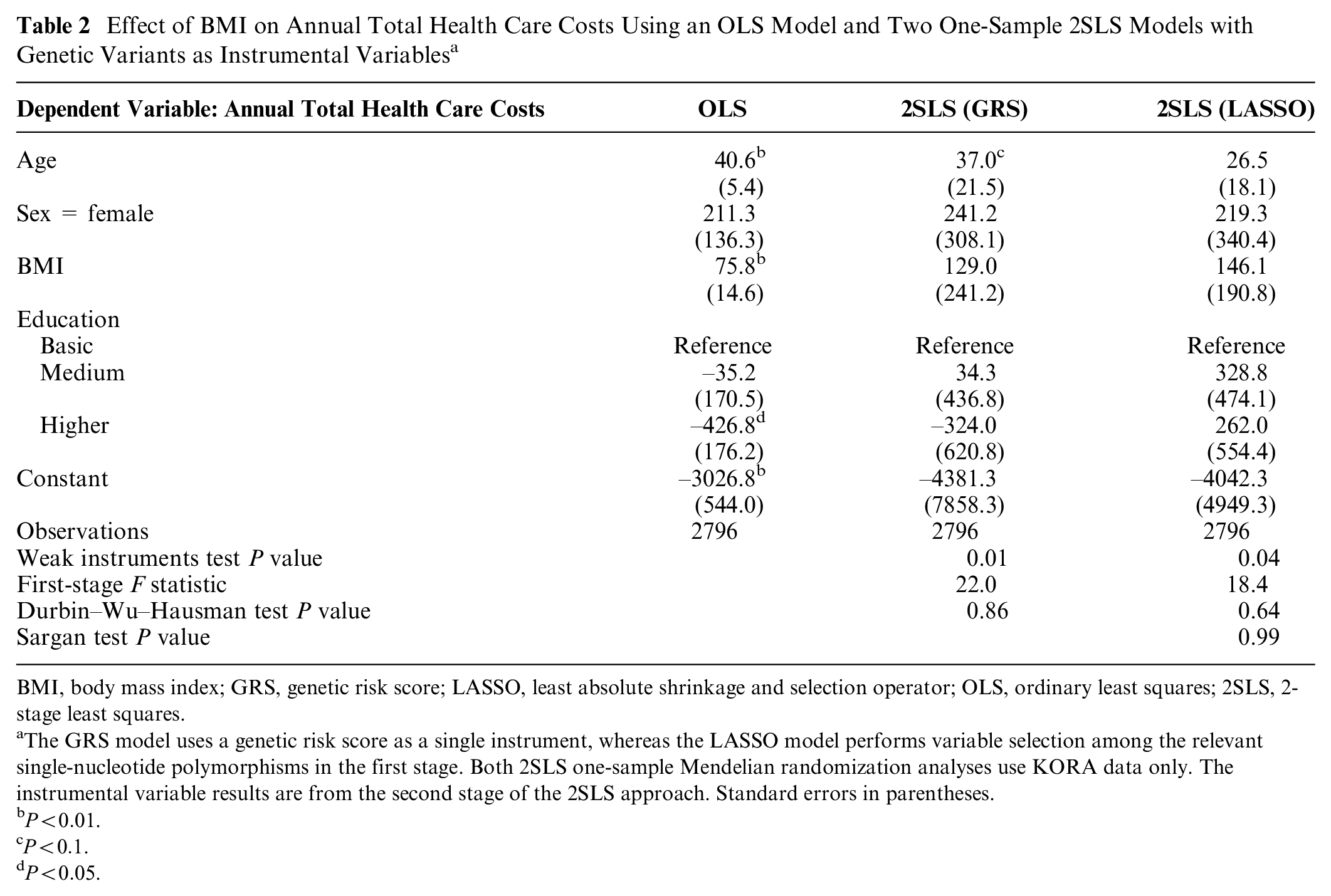
BMI, body mass index; GRS, genetic risk score; LASSO, least absolute shrinkage and selection operator; OLS, ordinary least squares; 2SLS, 2-stage least squares.

The GRS model uses a genetic risk score as a single instrument, whereas the LASSO model performs variable selection among the relevant single-nucleotide polymorphisms in the first stage. Both 2SLS one-sample Mendelian randomization analyses use KORA data only. The instrumental variable results are from the second stage of the 2SLS approach. Standard errors in parentheses.

$P < 0.01$ .

$P < 0.1$ .

$P < 0.05$ .

In both 2SLS analyses, we find little evidence of weak instruments, because the weak instruments test P value is <0.05 in both cases and the F statistics are above the traditional threshold of 10.³⁹ The Durbin–Wu–Hausman test, however, suggests no strong evidence of differences between the OLS and IV estimates.

Two-Sample MR

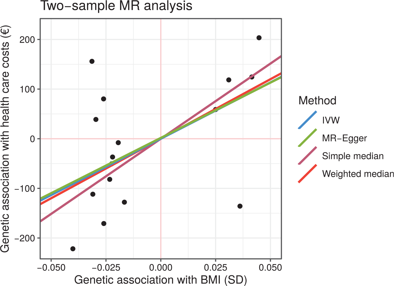
In Figure 2 and Table 3, we present the effect estimates from the two-sample MR analyses. All 4 methods find a higher causal effect than the 2SLS approaches. For example, the MR Egger method estimates a causal effect of €397.7 (95% CI, –795 to 1590) for a 1-unit increase in BMI. These effects increase from €405.1 (95% CI, –87 to 898) for the IVW method, to €428.3 (95% CI, –295 to 1152) for the weighted median, to €540.8 (95% CI, –192 to 1273) for the simple median method. However, all 95% confidence intervals are very wide, and the results cannot be considered statistically significant. The absence of pleiotropic effects is supported by the MR Egger intercept test (P = 0.99).

Table 3

Effect of BMI on Annual Total Health Care Costs Estimated by Two-Sample MR Using Simple Median, Weighted Median, IVW, and MR Egger Methods^a

Two-Sample MR
Method	Estimate	95% CI	P Value
Simple median	540.8	−191.6 to 1273.2	0.15
Weighted median	428.3	−294.9 to 1151.5	0.25
IVW	405.1	−87.3 to 897.5	0.11
MR Egger	397.7	−794.8 to 1590.2	0.51
MR Egger intercept	0.3	−42.7 to 43.0	0.99

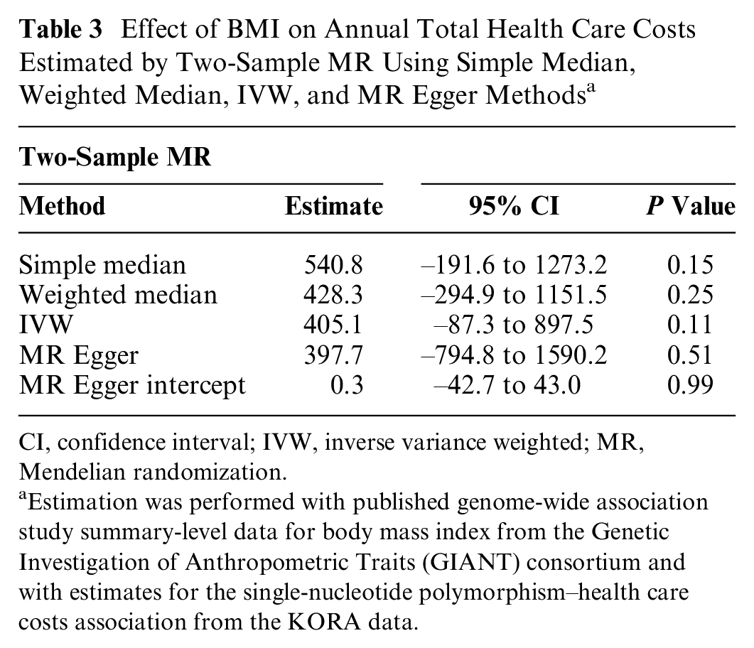
CI, confidence interval; IVW, inverse variance weighted; MR, Mendelian randomization.

Estimation was performed with published genome-wide association study summary-level data for body mass index from the Genetic Investigation of Anthropometric Traits (GIANT) consortium and with estimates for the single-nucleotide polymorphism–health care costs association from the KORA data.

Figure 2

Plot of the gene–outcome v. gene–exposure regression coefficients for body mass index across different two-sample Mendelian randomization methods. Each point represents a single-nucleotide polymorphism. Some outliers are not shown.

Meta-Analysis

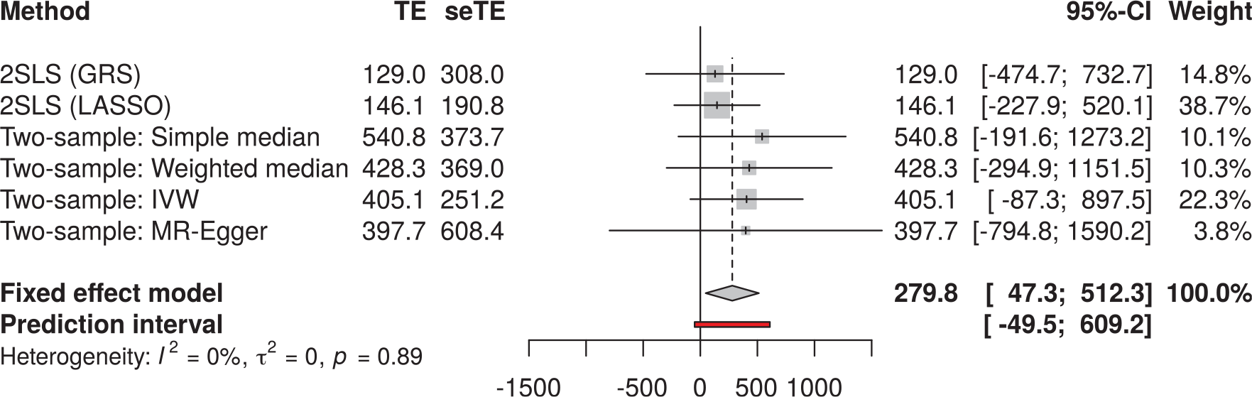
The meta-analysis of the 6 individual analyses (one-sample 2SLS with GRS, one-sample 2SLS with LASSO, two-sample simple median, two-sample weighted median, two-sample IVW, two-sample MR Egger) estimates a total causal effect of €279.8 for a 1-unit increase in BMI on annual total health care costs (see Figure 3). The 95% confidence interval for this effect is 47.3 to 512.3, and the complete prediction interval is –49.5 to 609.2. Most weight is assigned to the 2SLS LASSO (38.7%) and IVW (22.3%) methods.

Figure 3

Meta-analysis of one-sample and two-sample Mendelian randomization (MR) causal estimates using individual single-nucleotide polymorphisms (SNPs) as instrumental variables. One-sample MR using both a genetic risk score (GRS) and least absolute shrinkage and selection operator (LASSO) variable selection was performed using the KORA data only. Two-sample MR using 4 different methods was performed with published genome-wide association study summary-level data for body mass index from the Genetic Investigation of Anthropometric Traits (GIANT) consortium and with estimates for the SNP–health care costs association from the KORA data.

Pleiotropy

In the PhenoScanner database, we found that some SNPs are relevant to obesity-related illnesses such as type 2 diabetes and high blood pressure. As in Böckerman et al.,¹⁵ we assume that the associations with obesity-related conditions occur because of the SNPs’ association with high BMI, but we cannot definitely rule out other pathways. The Sargan test does not provide evidence of pleiotropic effects in the 2SLS LASSO model (see P values in Table 2). In addition, the absence of pleiotropic effects is supported by the MR Egger intercept test (P = 0.99; see Table 3).

Nonlinearity

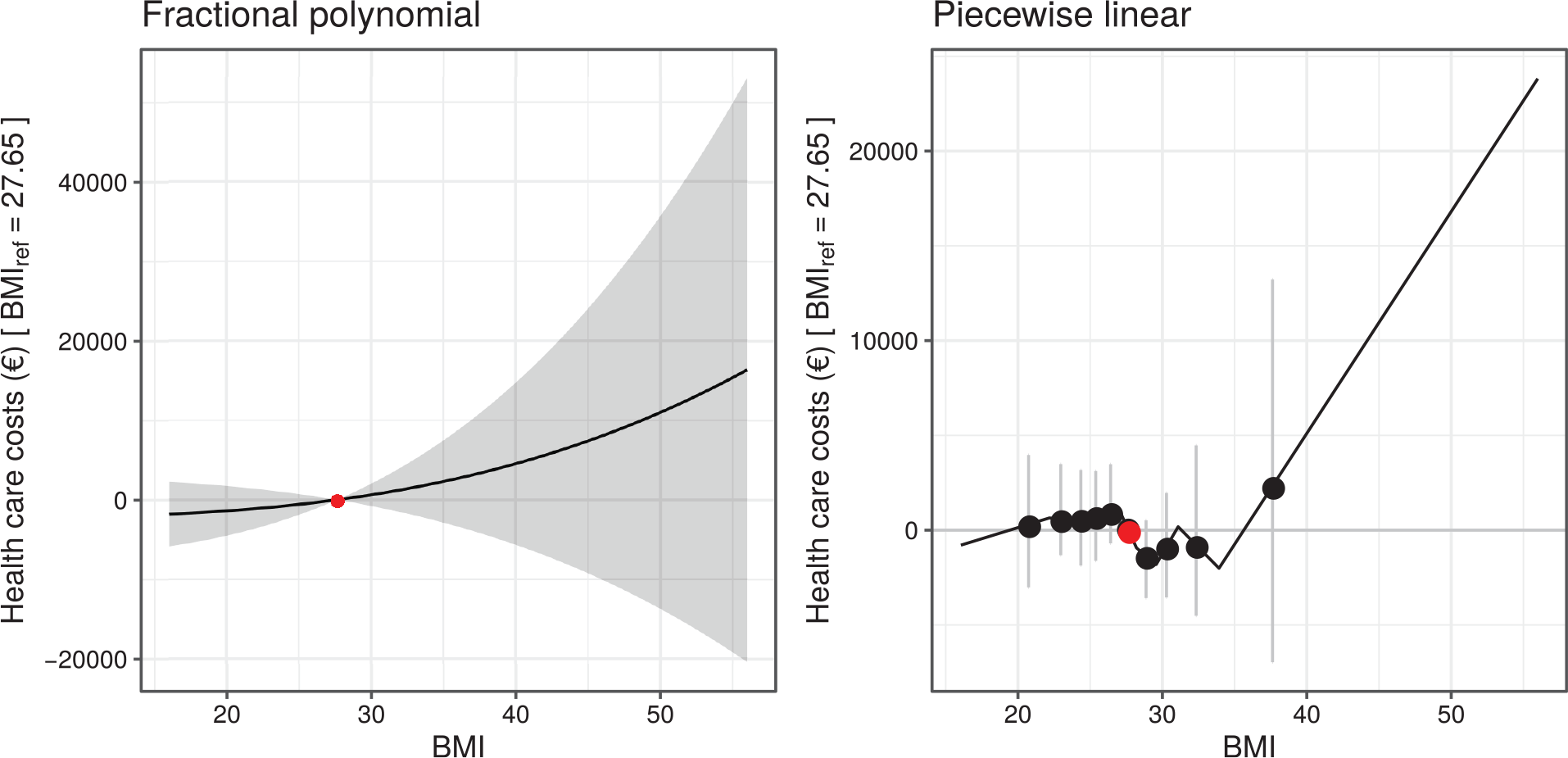
There was no strong evidence that the association between BMI and health care costs was nonlinear (see Figure 4), with the quadratic test yielding a P value of 0.52 (fractional polynomial test P = 0.59, Cochran Q test P = 0.62). The best-fitting fractional polynomial of degree 1 for the relationship between BMI and health care costs had power 3, and there was no evidence to suggest a fractional polynomial of degree 2 fitted the data better (P = 0.87).

Figure 4

Exposure–outcome relationships for body mass index (BMI) with health care costs estimated using the fractional polynomial and piecewise linear methods. The red points represent the reference point of BMI of 27.65 kg/m². Gray areas and lines represent the 95% confidence intervals.

Discussion

This study is one of the first that uses an MR approach to estimate the marginal health care costs of a prevalent clinical condition. MR offers new opportunities for reliable causal inference in health economic research within the framework of observational research designs. The recent advent of affordable GWASs provides an exciting opportunity to understand with far greater precision the genetic factors that influence variation in psychological, social, and health-related traits. Even an incomplete understanding of the genetic architecture of a trait could be a boon for social scientists; the presence of genetic variants can be detected with high reliability, thus allowing to identify or clarify the actual biological mechanisms that underlie social and health behaviors.⁶⁸

Using MR, our findings indicate that a 1-unit increase in BMI increases total medical spending by €279.8, based on the meta-analysis of several MR methods. The OLS model, which does not use instrumental variables, only finds additional spending of €75.8. This demonstrates that an MR study with genetic instruments may detect more hidden bias than a non-IV analysis, leading to higher estimated effects. It is important to note that OLS estimates average treatment effects, whereas IV estimates local average treatment effects. This may partially account for the differences in the effect estimates.⁶⁹ Our study results are in a similar direction to those of Cawley and Meyerhoefer,⁸ Black et al.,¹³ and Kinge and Morris,¹⁴ which imply much higher costs of obesity in the IV analysis compared with the non-IV analysis. These studies use the BMI of the respondent’s oldest child as instrument and report that the IV estimate for the association between BMI and health care costs is between 2 and 4 times higher than in the non-IV approach, about the same magnitude that we find. However, as it is likely that, because of shared environmental exposures, a child’s BMI is correlated with relevant covariates,⁷⁰ the use of such non- or quasi-genetic IVs is found to be controversial and might lead to biased estimates as well.

Another advantage of our data is that the height and weight measurements of individuals in the KORA sample were performed by trained staff. This is more accurate than self-reported measurements where people tend to underestimate their weight and overestimate their height, resulting in an underestimation in BMI.⁷¹

Because participants in our study were asked to self-report their health service usage over the past 3 to 12 months, recall bias cannot be excluded, and it is expected that total utilization and costs are underestimated. Health care utilization was priced using average reference value; therefore, actual costs might deviate. However, this should not influence the validity of the study results because its effect on relative excess cost estimates is expected to be rather small.⁷² In addition, we were unable to consider cost categories such as presenteeism, premature death, or out-of-pocket payments for medication. In total, these limitations led to an underestimation of total health care costs that might also lead to an underestimation of marginal costs—which of course applies for both the OLS and one-sample/two-sample MR.

Other studies found similar results. Within the BMI range of 25 to 45 kg/m², a study in the United States by Wang et al.⁷³ described an increase in medical and pharmaceutical costs of $202.3 per BMI unit. A review of 75 international studies by Kent et al.⁷⁴ reported a median increase in mean total annual health care costs of 36% for obese individuals compared with individuals of healthy weight. However, all these studies rely on traditional non-IV estimations and might underestimate the true effect.

A major limitation of our study is the low statistical power of the one-sample approach. Making anticonservative assumptions (i.e., that the true causal effect is the MR effect reported in the study, with an observational estimate as per the OLS estimate), power is 0.44.⁷⁵ This low power is mainly because of the small sample size, large variance in health care costs, and the weak SNP–BMI association. The differing effect size of covariates and larger confidence intervals between OLS and 2SLS models may also be attributable to low power. To reach a power level of 0.8, the sample size would need to be at least 12,000.

Having weak or invalid instruments can be a problem in MR analysis. This is a common problem in MR because behavioral traits are mainly affected by numerous genes with small effects.⁶⁸ Davies et al.⁵² show that 2SLS is especially vulnerable to weak instrument bias in MR and propose the limited information maximum likelihood and the continuously updating estimator as unbiased alternatives to 2SLS. However, these methods are difficult to implement and interpret. For this reason, we used the GRS and adaptive LASSO variable selection in the first state of 2SLS to rule out invalid and weak instruments. The SNPs we used have been discovered in GWAS and should be well founded, but it is also possible that there might be some direct effect that does not operate through a high BMI because some SNPs are linked to obesity-related illnesses.

The Durbin–Wu–Hausman test P value suggests no significant difference between OLS and IV estimates for the one-sample methods. However, the effects being estimated by the 2 methods may not be the same—the MR estimate reflects the effects of lifelong perturbations in the risk factor, whereas OLS regression results may reflect more acute effects.⁷⁶ According to Burgess and Thompson,⁷⁷ it would be fallacious to assume that a nonsignificant result means the OLS estimate is unconfounded. MR estimates are almost always less precise and have wider confidence intervals than OLS regression, so tests for difference often have low statistical power.

It must also be noted that the KORA F4 study was part of the GWAS consortium that discovered the relevant SNPs for BMI in the study by Locke et al.²⁶ Because the same data were used at the GWAS discovery stage and in our analysis, it is possible that chance correlation between SNPs and confounders can lead to overestimation of the SNP–trait effect.⁷⁸ This is the so-called winner’s curse or Beavis effect.⁷⁹ However, the KORA F4 study was only a small fraction of the more than 300,000 individuals in this GWAS, so it should not strongly bias our analysis. Furthermore, this problem almost exclusively affects the one-sample analysis.

Burgess et al.⁸⁰ note that instrumental variable estimates using a linear model may not reflect causal effects for large changes in the exposure. In our case, we find the relationship between BMI and costs approximately linear, and therefore the linear model is justified.

In the 2SLS estimator, we assume normal distribution of cost data, which is not present because of skewness, positivity, and heavy tails. This can also affect the validity of the standard errors and confidence intervals.^81,82 Still, the use of a linear model is justified because the skewness and tail distribution are not extreme, and the large sample size guarantees near-normality of sample means because of the central limit theorem.⁸³

In conclusion, we have shown that MR can be a viable tool in health economic analyses. We found more than 3 times higher costs for a 1-unit BMI unit increase in our IV model than in the OLS model. Because the association of genetic variants with BMI is still weak, and the sample size of our one-sample analysis is very low, the results have to be interpreted carefully.

Footnotes

Acknowledgements

We thank Konstantin Strauch, Thomas Meitinger, Harald Grallert, Christine Meisinger, and Annette Peters for providing the data.

The author(s) declared no potential conflicts of interest with respect to the research, authorship, and/or publication of this article.

The author(s) received no financial support for the research, authorship, and/or publication of this article.

ORCID iD

Christoph F. Kurz

Supplemental Material

Supplementary material for this article is available on the Medical Decision Making Web site at .

References

Wang

McPherson

Marsh

Gortmaker

Brown

. Health and economic burden of the projected obesity trends in the USA and the UK. Lancet. 2011;378(9793):815–25.

NCD Risk Factor Collaboration. Trends in adult body-mass index in 200 countries from 1975 to 2014: a pooled analysis of 1698 population-based measurement studies with 19.2 million participants. Lancet. 2016;387(10026):1377–96.

Willett

Stampfer

Colditz

Manson

. Adiposity as compared with physical activity in predicting mortality among women. N Engl J Med. 2004;351(26):2694–703.

World Health Organization. Obesity: Preventing and Managing the Global Epidemic. Geneva, Switzerland: World Health Organization; 2000.

Yang

Manolio

Pasquale

, et al. Genome partitioning of genetic variation for complex traits using common SNPs. Nat Genet. 2011;43(6):519.

Maes

HHM

Neale

and Eaves

. Genetic and environmental factors in relative body weight and human adiposity. Behav Gen. 1997;27(4):325–51.

Drummond

Sculpher

Claxton

Stoddart

Torrance

. Methods for the Economic Evaluation of Health Care Programmes. Oxford, UK: Oxford University Press; 2015.

Cawley

Meyerhoefer

. The medical care costs of obesity: an instrumental variables approach. J Health Econ. 2012;31(1):219–30.

Finkelstein

Trogdon

Cohen

Dietz

. Annual medical spending attributable to obesity: payer-and service-specific estimates. Health Aff. 2009;28(5):w822–w831.

10.

Trasande

Liu

Fryer

Weitzman

. Effects of childhood obesity on hospital care and costs, 1999–2005. Health Aff. 2009;28(4):w751–w760.

11.

Carreras-Torres

Johansson

Haycock

, et al. Role of obesity in smoking behaviour: Mendelian randomisation study in UK biobank. BMJ. 2018;361:k1767.

12.

Dare

Mackay

Pell

. Relationship between smoking and obesity: a cross-sectional study of 499,504 middle-aged adults in the UK general population. PLoS One. 2015;10(4):e0123579.

13.

Black

Hughes

Jones

. The health care costs of childhood obesity in Australia: an instrumental variables approach. Econ Hum Biol. 2018;31:1–13.

14.

Kinge

Morris

. The impact of childhood obesity on health and health service use. Health Serv Res. 2018;53(3):1621–43.

15.

Böckerman

Cawley

Viinikainen

, et al. The effect of weight on labor market outcomes: an application of genetic instrumental variables. Health Econ. 2019;28(1):65–77.

16.

Thomas

Conti

. Commentary: the concept of ‘mendelian randomization’. Int J Epidemiol. 2004;33(1):21–25.

17.

Ebrahim

Smith

. Mendelian randomization: can genetic epidemiology help redress the failures of observational epidemiology? Hum Genet. 2008;123(1):15–33.

18.

Dixon

Smith

von Hinke

Davies

Hollingworth

. Estimating marginal healthcare costs using genetic variants as instrumental variables: Mendelian randomization in economic evaluation. Pharmacoeconomics. 2016;34(11):1075–86.

19.

Ding

Lehrer

Rosenquist

Audrain-McGovern

. The impact of poor health on academic performance: new evidence using genetic markers. J Health Econ. 2009;28(3):578–97.

20.

Fletcher

Lehrer

. Genetic lotteries within families. J Health Econ. 2011;30(4):647–59.

21.

Norton

Han

. Genetic information, obesity, and labor market outcomes. Health Econ. 2008;17(9):1089–104.

22.

Cawley

Han

Norton

. The validity of genes related to neurotransmitters as instrumental variables. Health Econ. 2011;20(8):884–8.

23.

Willage

. The effect of weight on mental health: new evidence using genetic IVs. J Health Econ. 2018;57:113–30.

24.

von Hinke

Smith

Lawlor

Propper

Windmeijer

. Genetic markers as instrumental variables. J Health Econ. 2016;45:131–48.

25.

Holle

Happich

Löwel

Wichmann

H-E

, for the MONICA/KORA Study Group. Kora-a research platform for population based health research. Gesundheitswesen. 2005;67(Suppl 1):19–25.

26.

Locke

Kahali

Berndt

, et al. Genetic studies of body mass index yield new insights for obesity biology. Nature. 2015;518(7538):197.

27.

Price

Patterson

Plenge

, et al. Principal components analysis corrects for stratification in genome-wide association studies. Nat Genet. 2006;38(8):904.

28.

Burgess

Thompson

Rees

JMB

Day

Perry

Ong

. Dissecting causal pathways using mendelian randomization with summarized genetic data: application to age at menarche and risk of breast cancer. Genetics. 2017;207(2):481–7.

29.

Seidl

Bowles

Bock

, et al. Fima–questionnaire for health-related resource use in an elderly population: development and pilot study. Gesundheitswesen. 2015;77(1):46–52.

30.

Wacker

Holle

Heinrich

, et al. The association of smoking status with healthcare utilisation, productivity loss and resulting costs: results from the population-based KORA F4 study. BMC Health Serv Res. 2013;13(1):278.

31.

Bock

Brettschneider

Seidl

, et al. Calculation of standardised unit costs from a societal perspective for health economic evaluation. Gesundheitswesen. 2015;77(1):53–61.

32.

Yengo

Sidorenko

Kemper

, et al. Meta-analysis of genome-wide association studies for height and body mass index in 700000 individuals of European ancestry. Hum Mol Genet. 2018;27(20):3641–9.

33.

Taylor

Davies

Ware

VanderWeele

Smith

Munafò

. Mendelian randomization in health research: using appropriate genetic variants and avoiding biased estimates. Econ Hum Biol. 2014;13:99–106.

34.

R Core Team. R: A Language and Environment for Statistical Computing. Vienna, Austria: R Foundation for Statistical Computing; 2019.

35.

Kleiber

Zeileis

. Applied Econometrics with R. New York: Springer-Verlag; 2008.

36.

Yavorska

Staley

. MendelianRandomization: Mendelian Randomization Package. R package version 0.4.1. 2019. Available from: https://CRAN.R-project.org/package=MendelianRandomization.

37.

Angrist

Krueger

. Instrumental variables and the search for identification: From supply and demand to natural experiments. J Eco Perspect. 2011;15(4):69–85.

38.

Smith

. Randomised by (your) god: robust inference from an observational study design. J Epidemiol Community Health. 2006;60(5):382–8.

39.

Stock

Yogo

. Testing for weak instruments in linear IV regression. In Identification and Inference for Econometric Models: Essays in Honor of Thomas Rothenberg. UK: Cambridge University Press; 2005.

40.

Teumer

. Common methods for performing mendelian randomization. Front Cardiovasc Med. 2018;5:51.

41.

Glymour

Tchetgen Tchetgen

Robins

. Credible mendelian randomization studies: approaches for evaluating the instrumental variable assumptions. Am J Epidemiol. 2012;175(4):332–9.

42.

Hausman

. Specification tests in econometrics. Econometrica. 1978;46:1251–71.

43.

Lawlor

. Commentary: two-sample mendelian randomization: opportunities and challenges. Int J Epidemiol. 2016;45(3):908.

44.

Wald

. The fitting of straight lines if both variables are subject to error. Ann Math Stat. 1940;11(3):284–300.

45.

Angrist

Krueger

. Split-sample instrumental variables estimates of the return to schooling. J Bus Econ Stat. 1995;13(2):225–35.

46.

Inoue

Solon

. Two-sample instrumental variables estimators. Rev Econ Stat. 2010;92(3):557–61.

47.

Zhao

Wang

Spiller

, et al. Two-sample instrumental variable analyses using heterogeneous samples. Stat Sci. 2019;34(2):317–33.

48.

Bowden

Smith

Haycock

Burgess

. Consistent estimation in mendelian randomization with some invalid instruments using a weighted median estimator. Genet Epidemiol. 2016;40(4):304–14.

49.

Bowden

Smith

Burgess

. Mendelian randomization with invalid instruments: effect estimation and bias detection through egger regression. Int J Epidemiol. 2015;44(2):512–25.

50.

Hemani

Zheng

Elsworth

, et al. The MR-base platform supports systematic causal inference across the human phenome. Elife. 2018;7:e34408.

51.

Swerdlow

Kuchenbaecker

Shah

, et al. Selecting instruments for mendelian randomization in the wake of genome-wide association studies. Int J Epidemiol. 2016;45(5):1600–16.

52.

Davies

Scholder

SHK

Farbmacher

Burgess

Windmeijer

Smith

. The many weak instruments problem and mendelian randomization. Stat Med. 2015;34(3):454–68.

53.

Bound

Jaeger

Baker

. Problems with instrumental variables estimation when the correlation between the instruments and the endogenous explanatory variable is weak. J Am Stat Assoc. 1995;90(430):443–50.

54.

Staiger

Stock

. Instrumental variables regression with weak instruments. Econometrica. 1997;65(3):557–86.

55.

Belloni

Chen

Chernozhukov

Hansen

. Sparse models and methods for optimal instruments with an application to eminent domain. Econometrica. 2012;80(6):2369–429.

56.

Kang

Zhang

Cai

Small

. Instrumental variables estimation with some invalid instruments and its application to mendelian randomization. J Am Stat Assoc. 2016;111(513):132–44.

57.

Windmeijer

Farbmacher

Davies

Smith

. On the use of the lasso for instrumental variables estimation with some invalid instruments. J Am Stat Assoc. 2019; 114(527):1339–1350.

58.

Zou

. The adaptive lasso and its oracle properties. J Am Stat Assoc. 2006;101(476):1418–29.

59.

Smith

. Commentary: Random allocation in observational data: how small but robust effects could facilitate hypothesis-free causal inference. Epidemiology. 2011;22:460–3.

60.

Palmer

Lawlor

Harbord

, et al. Using multiple genetic variants as instrumental variables for modifiable risk factors. Stat Met Med Res. 2012;21(3):223–42.

61.

Viechtbauer

. Conducting meta-analyses in R with the metafor package. J Stat Soft. 201;36(3):1–48.

62.

Lawlor

Harbord

Sterne

JAC

Timpson

Smith

. Mendelian randomization: using genes as instruments for making causal inferences in epidemiology. Stat Med. 2008;27(8):1133–63.

63.

VanderWeele

Tchetgen Tchetgen

Cornelis

Kraft

. Methodological challenges in mendelian randomization. Epidemiology. 2014;25(3):427.

64.

Staley

Blackshaw

Kamat

, et al. Phenoscanner: a database of human genotype–phenotype associations. Bioinformatics. 2016;32(20):3207–9.

65.

Sargan

. The estimation of economic relationships using instrumental variables. Econometrica. 1958;26:393–415.

66.

Laxy

Stark

Peters

Hauner

Holle

Teuner

. The non-linear relationship between BMI and health care costs and the resulting cost fraction attributable to obesity. Int J Environ Res Public Health. 2017;14(9):984.

67.

Staley

Burgess

. Semiparametric methods for estimation of a nonlinear exposure-outcome relationship using instrumental variables with application to Mendelian randomization. Genet Epidemiol. 2017;41(4):341–52.

68.

Chabris

Lee

Benjamin

, et al. Why it is hard to find genes associated with social science traits: theoretical and empirical considerations. Am J Publ Health. 2013;103(Suppl 1):S152–66.

69.

Imbens

Angrist

. Identification and estimation of local average treatment effects. Econometrica. 1994;62(2):467–75.

70.

Dubois

Kyvik

Girard

, et al. Genetic and environmental contributions to weight, height, and BMI from birth to 19 years of age: an international study of over 12,000 twin pairs. PLoS One. 2012;7(2):e30153.

71.

Gorber

Tremblay

Moher

Gorber

. A comparison of direct vs. self-report measures for assessing height, weight and body mass index: a systematic review. Obesity Rev. 2007;8(4):307–26.

72.

Evans

Crawford

. Patient self-reports in pharmacoeconomic studies. Pharmacoeconomics. 1999;15(3):241–56.

73.

Wang

McDonald

Bender

Reffitt

Miller

Edington

. Association of healthcare costs with per unit body mass index increase. J Occupat Environ Med. 2006;48(7):668–74.

74.

Kent

Fusco

Gray

Jebb

Cairns

Mihaylova

. Body mass index and healthcare costs: a systematic literature review of individual participant data studies. Obesity Rev. 2017;18(8):869–79.

75.

Brion

M-JA

Shakhbazov

Visscher

. Calculating statistical power in mendelian randomization studies. Int J Epidemiol. 2012;42(5):1497–501.

76.

Davies

Holmes

Smith

. Reading mendelian randomisation studies: a guide, glossary, and checklist for clinicians. BMJ. 2018;362:k601.

77.

Burgess

Thompson

. Mendelian Randomization: Methods for Using Genetic Variants in Causal Estimation. London, UK: Chapman and Hall/CRC; 2015.

78.

Haycock

Burgess

Wade

Bowden

Relton

Smith

. Best (but oft-forgotten) practices: the design, analysis, and interpretation of mendelian randomization studies. Am J Clin Nutr. 2016;103(4):965–78.

79.

Göring

HHH

Terwilliger

Blangero

. Large upward bias in estimation of locus-specific effects from genomewide scans. Am J Hum Genet. 2001;69(6):1357–69.

80.

Burgess

Davies

Thompson

. Instrumental variable analysis with a nonlinear exposure–outcome relationship. Epidemiology. 2014;25(6):877.

81.

Guo

Kang

Cai

Small

. Confidence intervals for causal effects with invalid instruments by using two-stage hard thresholding with voting. J Royal Stat Soc B. 2018;80(4):793–815.

82.

Kang

Peck

Keele

. Inference for instrumental variables: a randomization inference approach. J Royal Stat Soc A. 2018;181(4):1231–54.

83.

Mihaylova

Briggs

O’Hagan

Thompson

. Review of statistical methods for analysing healthcare resources and costs. Health Econ. 2011;20(8):897–916.