A new perspective and extension of the Gaussian Filter

Abstract

The Gaussian Filter (GF) is one of the most widely used filtering algorithms; instances are the Extended Kalman Filter, the Unscented Kalman Filter and the Divided Difference Filter. The GF represents the belief of the current state by a Gaussian distribution, whose mean is an affine function of the measurement. We show that this representation can be too restrictive to accurately capture the dependences in systems with nonlinear observation models, and we investigate how the GF can be generalized to alleviate this problem. To this end, we view the GF as the solution to a constrained optimization problem. From this new perspective, the GF is seen as a special case of a much broader class of filters, obtained by relaxing the constraint on the form of the approximate posterior. On this basis, we outline some conditions which potential generalizations have to satisfy in order to maintain the computational efficiency of the GF. We propose one concrete generalization which corresponds to the standard GF using a pseudo measurement instead of the actual measurement. Extending an existing GF implementation in this manner is trivial. Nevertheless, we show that this small change can have a major impact on the estimation accuracy.

Keywords

Gaussian Filtering Bayesian estimation Kalman Filtering variational inference KL-divergence

1. Introduction

Decision making requires knowledge of some variables of interest. In the vast majority of real-world problems, these variables are latent; that is, they cannot be observed directly and must be inferred from available measurements. To maintain an up-to-date belief over the latent variables, past measurements have to be fused continuously with incoming measurements. This process is called filtering and its applications range from robotics to estimating a communication signal using noisy measurements (Anderson and Moore, 1979).

1.1. Dynamical systems modeling

Dynamical systems are typically modeled in a state–space representation, which means that the state is chosen such that the following two statements hold. First, the current observation depends only on the current state. Second, the next state of the system depends only on the current state. These assumptions can be visualized by the belief network shown in Figure 1.

Fig. 1.

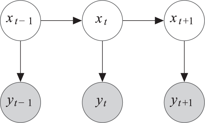
The belief network which characterizes the evolution of the state $x_{t}$ and the observation $y_{t}$ .

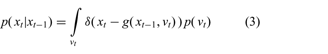
A stationary system can be characterized by two functions. The process model

x_{t} = g (x_{t - 1}, v_{t})

(1)

describes the evolution of the state $x_{t}$ . Without loss of generality, we can assume the noise $v_{t}$ to be drawn from a Gaussian distribution with zero mean and unit variance, since it can always be mapped onto any other distribution inside of the nonlinear function $g (\cdot)$ . The observation model

y_{t} = h (x_{t}, w_{t})

(2)

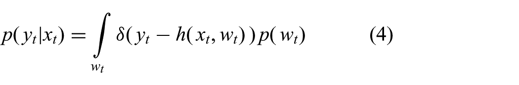
describes how a measurement is produced from the current state. Following the same reasoning as above, we assume the noise $w_{t}$ to be Gaussian with zero mean and unit variance. The process and observation models can also be represented by distributions. The distributional forms of both models are implied by their functional form

p (x_{t} | x_{t - 1}) = \int_{v_{t}} δ (x_{t} - g (x_{t - 1}, v_{t})) p (v_{t})

(3)

p (y_{t} | x_{t}) = \int_{w_{t}} δ (y_{t} - h (x_{t}, w_{t})) p (w_{t})

(4)

where $δ$ is the Dirac delta function, and the notation $\int_{x} (\cdot)$ is used as an abbreviation for $\int_{- \infty}^{\infty} (\cdot) dx$ . While both representations contain the exact same information, sometimes one is more convenient than the other.

1.2. Exact filtering

The desired posterior distribution over the current state $p (x_{t} | y_{1 : t})$ can be computed recursively from the distribution over the previous state $p (x_{t - 1} | y_{1 : t - 1})$ . This recursion can be written in two steps: a prediction step

p (x_{t} | y_{1 : t - 1}) = \int_{x_{t - 1}} p (x_{t} | x_{t - 1}) p (x_{t - 1} | y_{1 : t - 1})

(5)

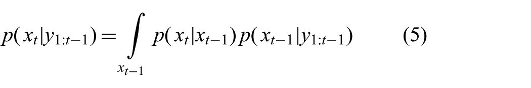
and an update step

p (x_{t} | y_{1 : t}) = \frac{p (y_{t} | x_{t}) p (x_{t} | y_{1 : t - 1})}{\int_{x_{t}} p (y_{t} | x_{t}) p (x_{t} | y_{1 : t - 1})} .

(6)

Kalman (1960) found the solution to these equations for linear process and observation models with additive Gaussian noise. However, filtering in nonlinear systems remains an important area of research. Exact solutions (Beneš, 1981; Daum, 1986) have been found for only a very restricted class of process and observation models. For more general dynamical systems, it is well known that the exact posterior distribution cannot be represented by a finite number of parameters (Kushner, 1967). Therefore, the need for approximations is evident.

1.3. Approximate filtering

Approximate filtering methods are typically divided into deterministic, parametric methods, such as the Unscented Kalman Filter (UKF) (Julier and Uhlmann, 1997) and the Extended Kalman Filter (EKF) (Sorenson, 1960), and stochastic, nonparametric methods such as the particle filter (Gordon et al., 1993). In this paper, we argue that there is a more fundamental division between filtering methods.

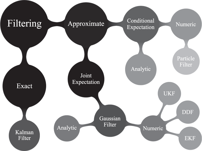
To the best of our knowledge, all existing filtering algorithms either compute expectations with respect to the conditional distribution $p (x_{t} | y_{1 : t})$ or with respect to the joint distribution $p (x_{t}, y_{t} | y_{1 : t - 1})$ . In Figure 2, we divide approximate filtering algorithms according this criterion. The computational power required to numerically compute expectations with respect to $p (x_{t} | y_{1 : t})$ increases exponentially with the state dimension, limiting the use of such methods to low-dimensional problems. In contrast, expectations with respect to the joint distribution $p (x_{t}, y_{t} | y_{1 : t - 1})$ can be computed efficiently, even for large state dimensions. In Section 3, we show how this fundamental difference arises.

Fig. 2.

A taxonomy of filtering algorithms.

Since conditional expectation methods suffer from the curse of dimensionality, we focus on joint expectation methods in this paper. To the best of our knowledge, all such methods approximate the true joint distribution $p (x_{t}, y_{t} | y_{1 : t - 1})$ with a Gaussian distribution $q (x_{t}, y_{t} | y_{1 : t - 1})$ and subsequently condition on $y_{t}$ , which is easy due to the Gaussian form. This approach is called the Gaussian Filter (GF), of which the well known EKF (Sorenson, 1960), the UKF (Julier and Uhlmann, 1997) and the Divided Difference Filter (DDF) (Nørgaard et al., 2000) are instances (Ito and Xiong, 2000; Särkkä, 2013; Wu et al., 2006). Morelande and Garcia-Fernandez (2013) show that for nonlinear dynamical systems, Gaussians can yield a poor fit to the true joint distribution $p (x_{t}, y_{t} | y_{1 : t - 1})$ , which in turn leads to bad filtering performance. To address this problem, we search for a more flexible representation of the belief that can accurately capture the dependences in the dynamical system, while maintaining the efficiency of the GF.

1.4. Contributions

The first contribution of this article is to provide a new perspective on the theory underlying Gaussian filtering. From this new perspective, the posterior belief obtained by the GF is seen as the solution of a constrained optimization problem. The objective of this optimization measures how well the approximate belief fits the exact posterior, and the constraint restricts the posterior belief to being Gaussian with the mean being an affine function of the measurement. This new perspective provides insights into the limitations and possible extensions of the GF. We show that the constraint on the form of the belief can lead to poor approximations of the exact posterior. This indicates that more accurate filters can be obtained by relaxing this constraint.

An analysis of how the constraint can be relaxed while maintaining the computational efficiency of the GF is the second main contribution of this article. This analysis provides the basis for generalizations of the GF. We provide one such generalization, but hope that this analysis will also stimulate further research in this direction.

The third contribution is one particular generalization of the GF, which amounts to using a pseudo measurement, that is, a nonlinear feature of the original measurement. This extension is straightforward and can readily be applied in standard GF implementations. We provide simulation examples indicating that this simple change can improve filtering performance significantly. These examples are chosen to highlight specific properties of the method, to illustrate the theoretical insights and to provide intuition on how the proposed technique can be applied to practical filtering problems.

While no full-scale robotic filtering example is presented herein, the results of this paper have already given rise to practical applications. In Wüthrich et al. (2016), a method for robustifying GFs against outliers using a pseudo measurement is presented, which is applied to three-dimensional (3D) object tracking using a depth sensor in Issac et al. (2016).

The present paper is an extension of preliminary results published in Wüthrich et al. (2015). The theoretical analysis has been significantly extended and is now contained in Sections 6, 7 and 8. Furthermore, two additional simulation experiments have been added in Sections 9.3 and 9.4 to further illustrate the practical relevance of the proposed method.

1.5. Outline

In Sections 2–4, we first review existing filtering methods, in particular the GF. Then, in Section 6, we view the GF as the solution to a constrained optimization problem. From this perspective, the GF is seen as a special case of a potentially much broader class of filters. In Section 7, we analyze how the GF could be generalized. Finally, in Section 8, we propose one possible extension of the GF and show that this generalization coincides with the GF using a pseudo measurement. Numerical simulations in Section 9 illustrate why using such pseudo measurements instead of the actual measurement can improve estimation accuracy significantly.

2. Approximate prediction

We start out with the distribution $p (x_{t - 1} | y_{1 : t - 1})$ computed in the previous time step. The representation of the beliefs might be parametric, for instance Gaussian, or it might be nonparametric, such as a set of samples. In any case, the goal is to find the prediction $p (x_{t} | y_{1 : t - 1})$ given the previous belief. When there is no closed form solution to (5), we have to settle for finding certain properties of the predicted belief $p (x_{t} | y_{1 : t - 1})$ instead of the full distribution. For all filtering algorithms we are aware of, these desired properties can be written as expectations

\int_{x_{t}} f (x_{t}) p (x_{t} | y_{1 : t - 1}) .

(7)

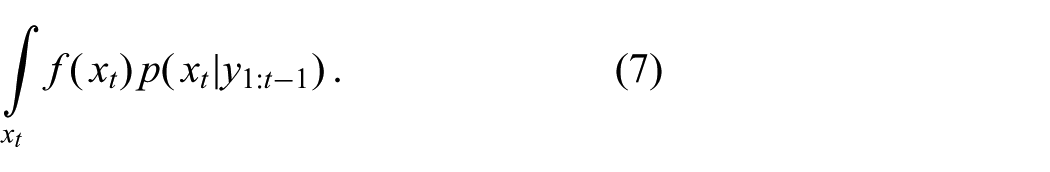
For instance with $f (x_{t}) = x_{t}$ , we obtain the mean $μ_{t}$ , and with $f (x_{t}) = (x_{t} - μ_{t}) (x_{t} - μ_{t})^{T}$ , we obtain the covariance. These expectations can then be used to find the parameters of an approximate distribution. A widely used approach is moment matching, where the moments of the approximate distribution are set to the moments of the exact distribution. We will analyze such methods in more detail below. What is important here is that we are always concerned with finding expectations of the form of (7).

We substitute (5) in (7) in order to write this expectation in terms of the last belief and the process model

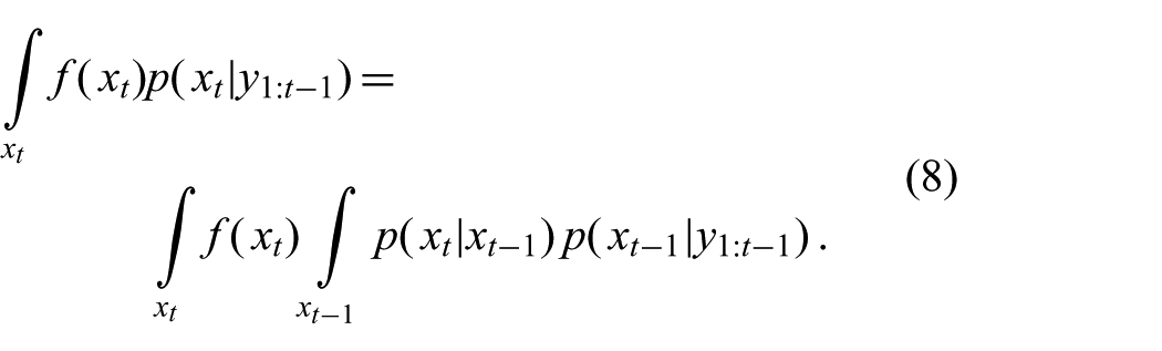
\begin{matrix} \int_{x_{t}} f (x_{t}) p (x_{t} | y_{1 : t - 1}) = \\ \int_{x_{t}} f (x_{t}) \int_{x_{t - 1}} p (x_{t} | x_{t - 1}) p (x_{t - 1} | y_{1 : t - 1}) . \end{matrix}

(8)

Substituting the distributional process model (3) and solving the integral over $x_{t}$ , which is easy due to the Dirac distribution $δ$ , we obtain

\begin{matrix} \int_{x_{t}} f (x_{t}) p (x_{t} | y_{1 : t - 1}) = \\ \int_{x_{t - 1}, v_{t}} f (g (x_{t - 1}, v_{t})) p (v_{t}) p (x_{t - 1} | y_{1 : t - 1}) . \end{matrix}

(9)

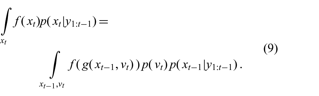
For certain process models $g (\cdot)$ and functions $f (\cdot)$ , it is possible to find a closed form solution. In general, however, this integral has to be computed numerically. Since $p (v_{t})$ is the Gaussian noise distribution and $p (x_{t - 1} | y_{1 : t - 1})$ is the previous belief in the representation of choice, it is generally possible to sample from these two distributions. This is crucial since it is a requirement for the application of Monte Carlo integration as well as deterministic integration methods.

Both types of methods approximate (9) by evaluating the integrand at different points and summing them up

\sum_{l = 1}^{L} w^{l} f (g (x_{t - 1}^{l}, v_{t}^{l}))

(10)

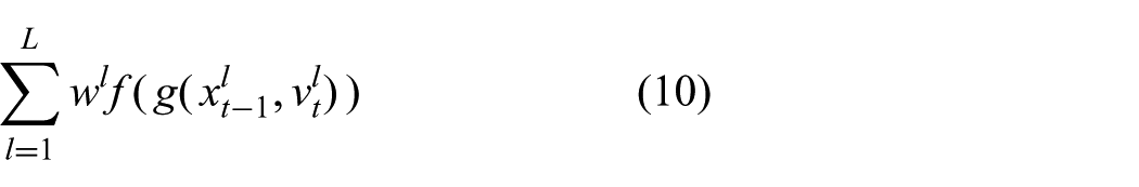
where L is the number of evaluations. The evaluation points ${(x_{t - 1}^{l}, v_{t}^{l})}_{l}$ and the weights $w^{l}$ depend on the integration scheme used.

2.1. Monte Carlo integration

In Monte Carlo integration, ${x_{t - 1}^{l}}_{l}$ are random samples drawn from $p (x_{t - 1} | y_{1 : t - 1})$ and ${v_{t}^{l}}_{l}$ are sampled from $p (v_{t})$ . The weights $w^{l} = 1 / L$ are uniform. The standard deviation of a Monte Carlo estimate, indicating its accuracy, is proportional to $\frac{1}{\sqrt{L}}$ , with L being the number of samples (Bishop, 2006; Owen, 2013). A key property of Monte Carlo methods is that the accuracy of the estimate does not depend on the dimension of the variable, in this case $x_{t}$ (Bishop, 2006; Owen, 2013).

2.2. Gaussian quadrature

Another possibility is to use deterministic numerical integration algorithms, such as Gaussian quadrature methods. In such methods, the weights $w^{l}$ and evaluation points ${(x_{t - 1}^{l}, v_{t}^{l})}_{l}$ are chosen such that the approximation is exact for polynomial integrands up to some degree. For instance, the standard unscented transform (Julier and Uhlmann, 1997) integrates polynomials up to degree 3 exactly and requires $2 d + 1$ evaluations, where d is the state dimension. For an overview of existing Gaussian quadrature methods we refer the interested reader to Wu et al. (2006). What is important here is that the number of function evaluations of such methods typically scales linearly or quadratically with the state dimension (Wu et al., 2006).

2.3. Conclusion

Which particular numeric integration method is used to compute the approximate expectations is inconsequential for the results presented in this paper. What is important here is that the numeric computation of expectations of the type (7) is tractable; that is, it does not suffer from the curse of dimensionality. As we will see shortly, this is unfortunately not the case in the update step.

3. Approximate update

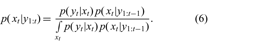
The goal of the update step is to obtain an approximation of the posterior $p (x_{t} | y_{1 : t})$ based on the belief $p (x_{t} | y_{1 : t - 1})$ , which has been computed in the prediction step.

3.1. Computation of conditional expectations

As for the prediction, when there is no exact solution to (6), we compute expectations with respect to the posterior $\int_{x_{t}} r (x_{t}) p (x_{t} | y_{1 : t})$ , where $r (\cdot)$ is an arbitrary function. We insert (6) to express this expectation in terms of the observation model and the predicted distribution

\int_{x_{t}} r (x_{t}) p (x_{t} | y_{1 : t}) = \frac{\int_{x_{t}} r (x_{t}) p (y_{t} | x_{t}) p (x_{t} | y_{1 : t - 1})}{\int_{x_{t}} p (y_{t} | x_{t}) p (x_{t} | y_{1 : t - 1})} .

(11)

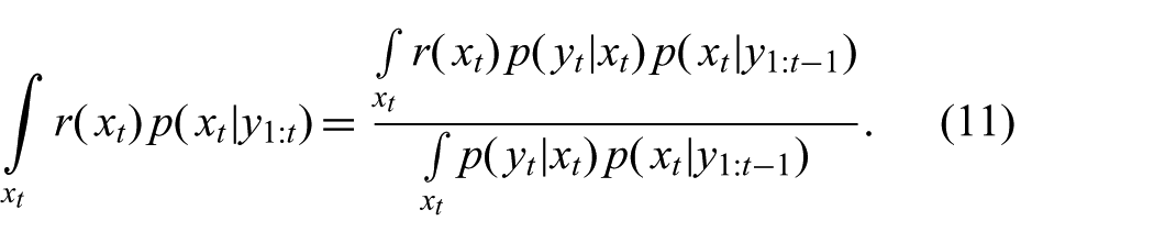
Both the numerator and the denominator can be written as

\int_{x_{t}} s (x_{t}) p (y_{t} | x_{t}) p (x_{t} | y_{1 : t - 1})

(12)

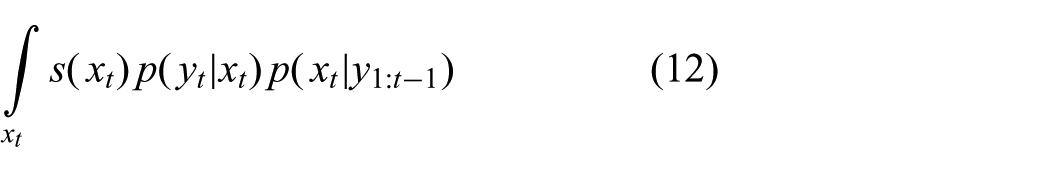
with $s (x_{t}) = r (x_{t})$ for the numerator and $s (x_{t}) = 1$ for the denominator. The update step thus amounts to computing expectations of the form of (12).

As in the prediction step, we can approximate this expectation either by sampling, which is used in Sequential Monte Carlo (Cappé et al., 2007; Gordon et al., 1993), or by applying deterministic methods such as Gaussian quadrature (Kushner and Budhiraja, 2000).

There is, however, a very important difference from the prediction step. We now need to compute the expectation of a function weighted with $p (y_{t} | x_{t})$ . This typically leads to the weights $p (y_{t} | x_{t}^{(l)})$ being small at most evaluation points ${x_{t}^{(l)}}$ , and the numeric integration therefore becomes very inaccurate. This problem is well known in importance sampling (Bishop, 2006; Owen, 2013). In particle filters, this effect is known as particle deprivation (Cappé et al., 2007).

Unfortunately, this effect becomes worse with increasing dimensionality. To see this, consider a simple example with a predictive distribution $p (x_{t} | y_{1 : t - 1}) = N (x_{t} | 0, I)$ and observation model $p (y_{t} | x_{t}) = N (y_{t} | x_{t}, I)$ . Both the state and measurement dimensions are equal to D. Computing the expected weight, that is, the expected value of the likelihood, yields

\begin{matrix} E [p (y_{t} | x_{t})] & = \int_{x_{t}, y_{t}} p (y_{t} | x_{t}) p (y_{t} | x_{t}) p (x_{t} | y_{1 : t - 1}) \\ = (2 \sqrt{π})^{- D} \end{matrix}

(13)

where $E [\cdot]$ is the expectation operator. That is, the expected weight decreases exponentially with the dimension D. In fact, it is well known that the computational demands of such methods increase exponentially with the state dimension (Bickel et al., 2008; Li et al., 2005; Owen, 2013); that is, they suffer from the curse of dimensionality. Thus, methods that rely on the computation of conditional expectations are restricted to dynamical systems which either have a simple structure such that expectations can be computed analytically, or are low dimensional such that numeric methods can be used.

3.2. Computation of joint expectations

There are a number of approaches which avoid computing such expectations with respect to the conditional distribution $p (x_{t} | y_{1 : t})$ . Instead, these methods find an approximate posterior while computing only expectations with respect to the joint distribution

\begin{matrix} \int_{x_{t}, y_{t}} d (x_{t}, y_{t}) p (y_{t}, x_{t} | y_{1 : t - 1}) = \\ \int_{x_{t}, y_{t}} d (x_{t}, y_{t}) p (y_{t} | x_{t}) p (x_{t} | y_{1 : t - 1}) \end{matrix}

(14)

where $d (\cdot)$ is some arbitrary function. Despite the apparent similarity between (12) and the right-hand side of (14), these terms are fundamentally different. In (12) the integration is performed with respect to $x_{t}$ only. The term $p (y_{t} | x_{t})$ plays the role of a weighting function, which is the cause of the computational inefficiency described in Section 3.1. In (14) however, the integral is taken with respect to both $x_{t}$ and $y_{t}$ . The term $p (y_{t} | x_{t})$ is now used for sampling instead of weighting, which avoids the mentioned inefficiency.

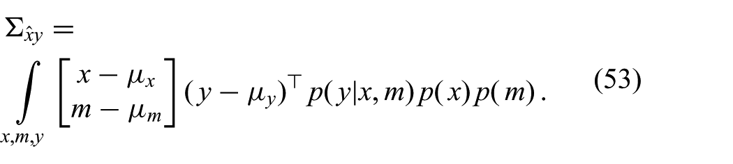
Inserting the observation model from (4) into the joint expectation above and solving the integral over $y_{t}$ yields

\begin{matrix} \int_{x_{t}, y_{t}} d (x_{t}, y_{t}) p (y_{t}, x_{t} | y_{1 : t - 1}) = \\ \int_{x_{t}, w_{t}} d (x_{t}, h (x_{t}, w_{t})) p (w_{t}) p (x_{t} | y_{1 : t - 1}) . \end{matrix}

(15)

This term has the same form as the expectation in the prediction step (9). It is an integral of some function with respect to probability densities from which we can sample. This allows us to approximate this expectation efficiently, even for high-dimensional states.

3.3. Conclusion

The insight of this section is that numeric computation of expectations with respect to the conditional distribution $p (x_{t} | y_{1 : t})$ suffers from the curse of dimensionality, whereas computing expectations with respect to the joint distribution $p (x_{t}, y_{t} | y_{1 : t - 1})$ is tractable.

Note that expectations with respect to the marginals $p (x_{t} | y_{1 : t - 1})$ and $p (y_{t} | y_{1 : t - 1})$ are a special case of an expectation with respect to the joint distribution and can be computed efficiently as well.

3.4. Notation

In the following theoretical Sections 4–8, we only consider a single update step. For ease of notation, we will not explicitly write the dependence on all previous observations $y_{1 : t - 1}$ anymore; it is however implicitly present in all distributions. All the remaining variables have the same time index t, which we can thus safely drop. For example, $p (x_{t}, y_{t} | y_{1 : t - 1})$ becomes $p (x, y)$ and $p (x_{t} | y_{1 : t})$ becomes $p (x | y)$ , etc.

It is important to keep in mind that the parameters computed in the following sections are also time varying; all computations described in the following are carried out at each time step.

4. The Gaussian Filter

The advantage in terms of computational complexity of joint expectation filters over conditional expectation filters comes at a price: the approximate posterior $q (x | y)$ must have a functional form such that its parameters can be computed efficiently from these joint expectations. To the best of our knowledge, all existing joint expectation filters solve this issue by approximating the true joint distribution $p (x, y)$ with a Gaussian distribution

q (x, y) = N ([\begin{matrix} x \\ y \end{matrix}] | [\begin{matrix} μ_{x} \\ μ_{y} \end{matrix}], [\begin{matrix} Σ_{xx} & Σ_{xy} \\ Σ_{yx} & Σ_{yy} \end{matrix}]) .

(16)

The parameters of this approximation are readily obtained by moment matching; that is, the moments of the Gaussian are set to the moments of the exact distribution

μ_{x} = \int_{x} xp (x)

(17a)

μ_{y} = \int_{y} yp (y)

(17b)

Σ_{xx} = \int_{x} (x - μ_{x}) (x - μ_{x})^{T} p (x)

(17c)

Σ_{yy} = \int_{y} (y - μ_{y}) (y - μ_{y})^{T} p (y)

(17d)

Σ_{xy} = \int_{x, y} (x - μ_{x}) (y - μ_{y})^{T} p (x, y) .

(17e)

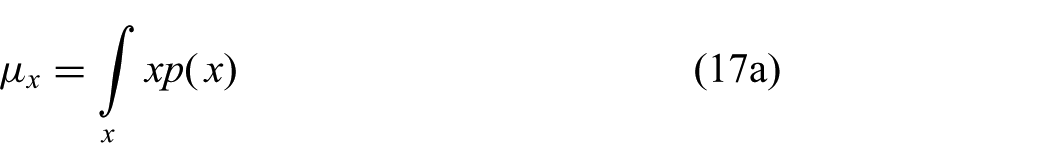
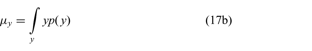
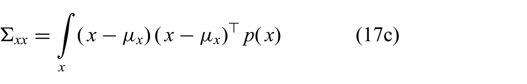
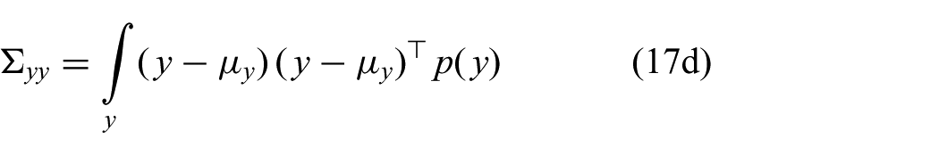
All of these expectations can be computed efficiently for reasons explained in the previous section.

After the moment matching step, we condition on y to obtain the desired posterior, which is a simple operation since the approximation is Gaussian

\begin{matrix} q (x | y) = \\ N (x | \underset{μ_{x | y}}{\underset{︸}{μ_{x} + Σ_{xy} Σ_{yy}^{- 1} (y - μ_{y})}}, \underset{Σ_{xx | y}}{\underset{︸}{Σ_{xx} - Σ_{xy} Σ_{yy}^{- 1} Σ_{xy}^{T}}}) . \end{matrix}

(18)

This approach is called the GF. Widely used filters such as the EKF (Sorenson, 1960) and the UKF (Julier and Uhlmann, 1997) can be seen as instances of the GF, differing only in the numeric integration method used for computing the expectations in (17). We refer the interested reader toWu et al. (2006), Särkkä (2013) and Ito and Xiong (2000) for more details on this point of view on Gaussian filtering.

4.1. Rank-deficient covariance matrix

Equation (18) involves a matrix inverse, which does not exist if $Σ_{yy}$ is rank deficient. While we use the matrix inverse for notational convenience, it should never be explicitly computed in an actual implementation. Instead, $μ_{x | y}$ and $Σ_{xx | y}$ can be formulated as solutions of linear systems. As shown in Appendix 1, these linear systems have unique solutions even if $Σ_{yy}$ is rank deficient. This point is particularly important for the ideas in this paper since we will augment the measurement vector with possibly redundant pseudo measurements, which can lead to a rank-deficient $Σ_{yy}$ .

4.2. Approximate integration schemes

The EKF solves the integrals (17) by linearizing the measurement function and then performing analytic integration. This approximation does not take the uncertainty in the estimate into account, which can lead to large errors and sometimes even divergence of the filter (Ito and Xiong, 2000; van der Merwe and Wan, 2003).

Therefore, approximations based on numeric integration methods are preferable in most cases (van der Merwe and Wan, 2003). Deterministic Gaussian integration schemes have been investigated thoroughly, resulting in filters such as the UKF (Julier and Uhlmann, 1997), the DDF (Nørgaard et al., 2000) and the Cubature Kalman Filter (Arasaratnam and Haykin, 2009). Alternatively, numeric integration can also be performed using Monte Carlo methods.

5. Problem statement and assumptions

While much effort has been devoted to finding accurate numeric integration schemes for GFs, there seems to be no joint expectation method using a non-Gaussian joint approximation $q (x, y)$ . The posterior (18), which we ultimately care about, is therefore Gaussian in the state x with the mean being an affine function of y. As we show in the experimental section, this form can be too restrictive to accurately capture the relationship between the measurement and the state in nonlinear settings. This leads to information about the state being discarded and ultimately to poor filtering performance.

This holds true even if we can compute the integrals accurately. The problem of a too restrictive parametric form of the belief is hence separate from the problem of numeric integration. In this article, we focus on the first problem and, to simplify analysis, we will assume that all numeric integrals with respect to the joint distribution can be computed with high precision. Nevertheless, the extensions proposed in this article are compatible with any of the numeric integration methods used in the standard GF. However, we do not analyze the impact of the integration inaccuracies on the proposed method.

6. A new perspective of the Gaussian Filter

In this section, we investigate whether it is possible to find a more general form of the approximate posterior $q (x | y)$ that still allows for efficient computation of the parameters. To this end, we write the problem of finding the the approximate distribution as an optimization problem.

6.1. Objective for the approximate joint distribution

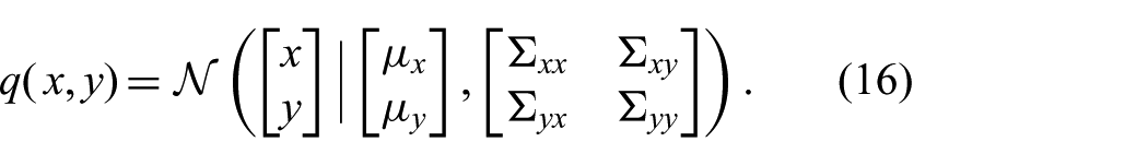
In the GF, the parameters of the Gaussian belief (16) are found by moment matching. For a Gaussian approximation $q (x, y)$ , moment matching is equivalent to minimizing the Kullback-Leibler (KL) divergence (Barber, 2012)

K L_{xy} [p (x, y) | q (x, y)] = \int_{x, y} \log (\frac{p (x, y)}{q (x, y)}) p (x, y) .

(19)

Hence, the GF can be understood as minimizing (19), subject to the constraint that $q (x, y)$ be Gaussian, and subsequently conditioning on y according to (18). We can write this formally as

\hat{q} (x, y) = \underset{q}{\arg \min} K L_{x} y [p (x, y) | q (x, y)]

(20a)

q (x, y) \in {N ([\begin{matrix} x \\ y \end{matrix}] | μ, \sum) : μ \in R^{k}, \sum \in R_{\geq 0}^{k}}

(20b)

\hat{q} (x | y) = \frac{\hat{q} (x, y)}{\int_{x} q (x, y)}

(20c)

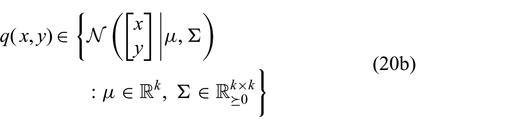
where k is the sum of the dimensions of x and y, and $R_{⪰} 0^{k \times k}$ is the set of all real positive semidefinite matrices of size $k \times k$ . Hence, following procedure (20) will merely retrieve the equations of the standard GF (17) and (18). However, from this perspective, the GF can be seen as just a special case of a potentially much broader class of filters, obtained by relaxing the constraint (20b). Still, we need to ensure that $q (x, y)$ has a form such that the subsequent conditioning (20c) can be carried out in closed form. Since this requirement is very restrictive, it is desirable to find an objective which is expressed in the approximate posterior $q (x | y)$ directly. This would remove the need for the conditioning step and the associated restriction on the form of the approximation.

6.2. Objective for the approximate posterior distribution

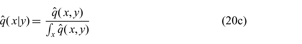
The goal is therefore to rewrite the constrained optimization with subsequent conditioning (20) as a constrained optimization directly yielding the same posterior $\hat{q} (x | y)$ as in (20c).

Any joint Gaussian distribution $q (x, y)$ can be written as a product of a conditional distribution $q (x | y)$ and a marginal distribution $α (y)$ , with $α (y)$ being Gaussian and $q (x | y)$ being Gaussian in x and the mean being an affine function in y (Bishop, 2006). Conversely, any Gaussian marginal distribution $α (y)$ and Gaussian conditional distribution $q (x | y)$ with linear dependence in y will yield a joint Gaussian distribution $q (x, y) = q (x | y) α (y)$ (Bishop, 2006). Hence, we can substitute $q (x, y)$ by $q (x | y) α (y)$ in (20a) and jointly optimize for $q (x | y)$ and $α (y)$ . The constraint (20b) on the joint distribution $q (x, y)$ then has to be replaced by the constraints on $q (x | y)$ and $α (y)$ . We thus translated procedure (20) into an equivalent optimization problem

{\hat{q} (x | y), \hat{α} (y)} = \underset{q, α}{\arg \min}, K L_{xy} [p (x, y) | q (x | y) (y)]

(21a)

q (x | y) \in {N (x | A [\begin{matrix} 1 \\ y \end{matrix}], C) : A \in R_{\geq 0}^{n \times (m + 1)}, C \in R_{\geq 0}^{n \times n}}

(21b)

α (y) \in {N (y | b, B) : b \in R^{m}, B \in R_{\geq 0}^{m \times m}

(21c)

where n is the dimension of x and m is the dimension of y. The new constraints (21b) and (21c) ensure that the joint distribution $q (x, y) = q (y | x) α (y)$ satisfies constraint (20b). Therefore, the optimization problem (21) is equivalent to (20).

The posterior $\hat{q} (x | y)$ is now obtained directly as the result of a constrained optimization, as desired. However, the optimization (21a) now has to be performed jointly in $q (x | y)$ and $α (x)$ . Fortunately, the optimization with respect to these two functions can be carried out independently, which can be seen by expanding (21a)

\begin{matrix} K L_{xy} [p (x, y) | q (x | y) α (y)] = \\ \int_{x, y} \log (\frac{p (x, y)}{α (y)}) p (x, y) - \int_{x, y} \log (q (x | y)) p (x, y) . \end{matrix}

(22)

Only the second term depends on the posterior $q (x | y)$ , which we are interested in. Therefore we can get rid of $α (y)$ in the optimization problem and finally obtain

\hat{q} (x | y) = \underset{q}{\arg \min} \overset{J [Q]}{\overset{︷}{\int_{x, y} - \log (q (x | y)) p (x, y)}}

(23a)

q (x | y) \in {N (x | A [\begin{matrix} 1 \\ y \end{matrix}], C) : A \in R^{n \times (m + 1)}, C \in R_{n_{0}}^{n \times n}} .

(23b)

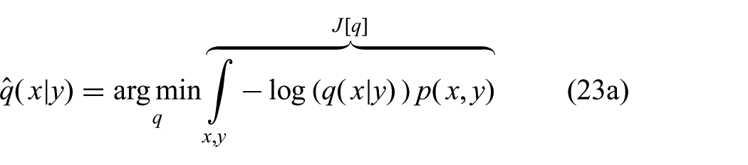
We have thus found a constrained optimization problem which yields the GF equations (17) and (18) as the solution. This point of view will serve as the basis for generalizations of the GF by relaxing (23b) in Section 7. First, we will look at the new objective (23a) in some more detail and make connections to alternative objective functions commonly used in filtering. We emphasize, however, that using (23a) as an objective is mainly justified by the fact that it yields the GF equations, and not by the following interpretations.

6.3. Connection to assumed density filtering

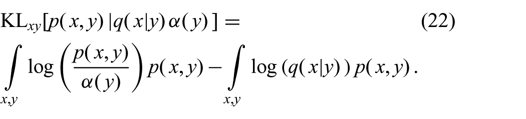
Above we showed that the GF minimizes the KL-divergence (19) between the exact joint distribution $p (x, y)$ and the approximate joint distribution $q (x, y)$ . However, what we are ultimately interested in is the fit between the exact posterior $p (x | y)$ and the approximate posterior $q (x | y)$

K L_{x} [p (x | y) | q (x | y)] = \int_{x} \log (\frac{p (x | y)}{q (x | y)}) p (x | y) .

(24)

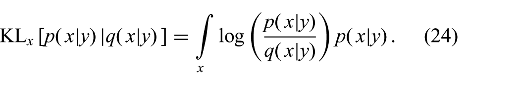
This objective is used in assumed density filtering (ADF) (Maybeck, 1979; Murphy, 2012) and expectation propagation (Minka, 2001). A drawback of such methods is their restriction to models where (24) can be optimized analytically. Approximating the integral (24) numerically is intractable in general since it requires the computation of expectations of the form of (11). Despite their differences in computational requirements, we shall make the connection here between the new objective (23a) and the commonly used objective (24).

By adding and subtracting $\log (p (x | y))$ in the integrand, and making use of the product rule $p (x, y) = p (x | y) p (y)$ , the objective function in (23a) can be rewritten as

\begin{matrix} J [q] = \int_{y} \int_{x} \log (\frac{p (x | y)}{q (x | y)}) p (x | y) p (y) \\ \underset{c}{\underset{︸}{- \int_{x, y} \log (p (x | y)) p (x, y)}} & . \end{matrix}

(25)

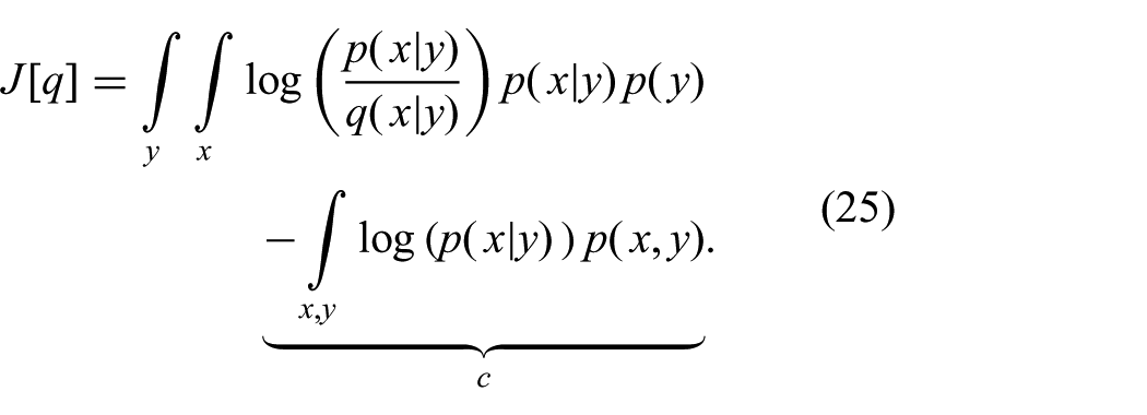
Using the definition of the KL-divergence (24), we can hence write the objective as

J [q] = E_{y} [K L_{x} [p (x | y) | q (x | y)]] + c

(26)

where $E [\cdot]$ is the expectation operator, and c does not depend on $q (x | y)$ and is therefore irrelevant. Hence, minimizing (23a) is equivalent to minimizing the expectation of the KL-divergence (24).

This means that the GF avoids computing the intractable conditional expectations in (24) by taking the expectation with respect to y. This leads to the objective (23a), where only expectations with respect to the joint distribution $p (x, y)$ have to be computed.

6.4. Information theoretic interpretation

The Shannon information content of an outcome z is defined as $- \log p (z)$ (MacKay, 2003). It can be interpreted as a measure of how surprised we are to observe z, given that we believe $p (z)$ to be the density of z. Similarly, $- \log q (x | y)$ is the degree of surprise when observing x, given that we have previously observed y and believe $q (x | y)$ to be the conditional density. A good state estimator should be as little surprised as possible if some oracle were to reveal the real state. Hence, intuitively it makes sense to minimize the expected degree of surprise

E_{xy} [- \log q (x | y)] = \int_{x, y} - \log q (x | y) p (x, y)

(27)

which is identical to (23a).

6.5. Properties of the objective

Further arguments why $J [q]$ in (23a) is a sensible objective are presented in the following.

First of all, if the approximate distribution $q (x | y)$ is flexible enough in y, then minimizing $J [q]$ is equivalent to minimizing (24) for each y separately, and we retrieve ADF. This is easy to see for a discrete variable y. Following (26), $J [q]$ can be written as

\sum_{i} K L_{x} [p (x | y = i) | q (x | y = i)] p (y = i) + c .

(28)

If there is no constraint linking $q (x | y = k)$ and $q (x | y = l)$ for any $k \neq l$ , then we can optimize each of the summands independently with respect to $q (x | y = i)$ , and we retrieve (24). A similar argument can be made for continuous y. In practice, the approximate distribution $q (x | y)$ will of course belong to some parametric family of distributions, and hence be subject to constraints in y. Nevertheless, this argument indicates that the more we relax the constraint (23b) in y, the closer we can expect the solution of (23a) to be to the solution of ADF.

If we remove the constraints in x as well, then the unconstrained minimum of (24) can be attained, which is at $q (x | y) = p (x | y)$ . Hence, if we were able to optimize (23a) without any constraints, then we would retrieve the exact posterior.

7. Conditions for generalizations of the Gaussian Filter

We have seen that the more we relax the constraint (23b), the closer we get to the solution of ADF (24) and to the exact posterior $p (x | y)$ . Therefore, we would like to find a family of distributions ${q (x | y, θ)}$ , with parameters $θ \in Θ$ , which is more general than (23b), but still allows for efficient optimization of (23a).

Unfortunately, this is a very difficult problem. In this section, we merely outline a few conditions that such a parametric family of distributions would have to fulfill. In Section 8, we shall then give one concrete example leading to a straightforward generalization of the GF.

7.1. General conditions

First of all, for the objective (23a) to be well defined, we require that $q (x | y, θ) > 0$ for all x and y for which $p (x, y) > 0$ . Since $p (x, y)$ is problem specific, and we would like to find a filtering algorithm which can be applied to any system, we require that $q (x | y, θ) > 0$ everywhere. This condition can be enforced by requiring the distribution to be of the form

q (x | y, θ) = c (y, θ) e^{u (x, y, θ)}

(29)

with $c (y, θ) > 0$ .

Secondly, $q (x | y, θ)$ has to integrate to one in x since it is a probability distribution. This condition can be met by setting $c (y, θ) = 1 / \int_{x} e^{u (x, y, θ)}$ , assuming that the integral exists. We can now write the approximate distribution as

q (x | y, θ) = \frac{e^{u (x, y, θ)}}{\int_{x} e^{u (x, y, θ)}}

(30)

where $u (\cdot)$ can be any function such that $\int_{x} e^{u (x, y, θ)}$ is finite for all y and all $θ \in Θ$ .

7.2. Conditions for efficiency

The question we will address in the following is what $u (\cdot)$ has to look like in order to obtain an efficient filtering algorithm.

The first condition for efficiency is that the objective function (23a) has to be convex in the parameters $θ$ of the approximate distribution (30). We therefore have to pick $u (\cdot)$ such that inserting (30) into (23a) yields an objective

\begin{matrix} J [q] = & \int_{y} \log (\int_{x} e^{u (x, y, θ)}) p (y) \\ - & \int_{x, y} u (x, y, θ) p (x, y) \end{matrix}

(31)

which is convex in $θ$ .

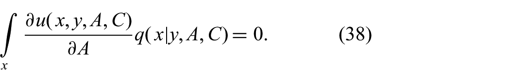
Given that (31) is convex, we can in principle find the optimal parameters by setting its derivative to zero and solving for $θ$ . We will now follow this procedure to see whether we need more conditions on $u (\cdot)$ to hold, in order to be able to find the optimal $θ$ .

Setting the derivative of (31) with respect to $θ$ to zero, we obtain a sufficient condition for optimality

\int_{x, y} \frac{\partial u (x, y, θ)}{\partial θ} p (x, y)

= \int_{y} \frac{\partial}{\partial θ} \log (\int_{x} e^{u (x, y, θ)}) p (y)

(32a)

= \int_{y} \frac{1}{\int_{x} e^{u (x, y, θ)}} \frac{\partial}{\partial θ} \int_{x} e^{u (x, y, θ)} p (y)

(32b)

= \int_{y} \frac{1}{\int_{x} e^{u (x, y, θ)}} \int_{x} e^{u (x, y, θ)} \frac{\partial u (x, y, θ)}{\partial θ} p (y)

(32c)

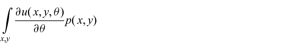
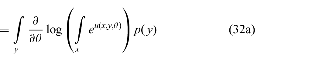
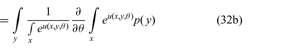
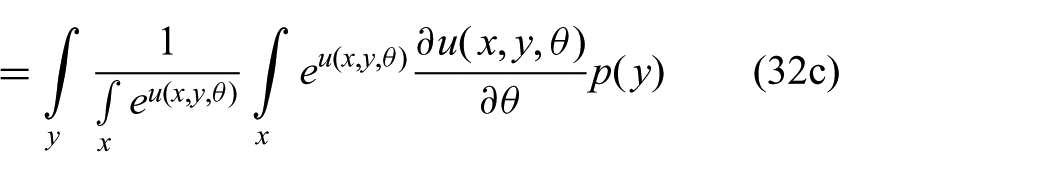
where we applied the chain rule in the step from (32a) to (32b) and from (32b) to (32c).

The left-most term in (32c) can be moved inside the integral, and by comparison with (30), we finally obtain

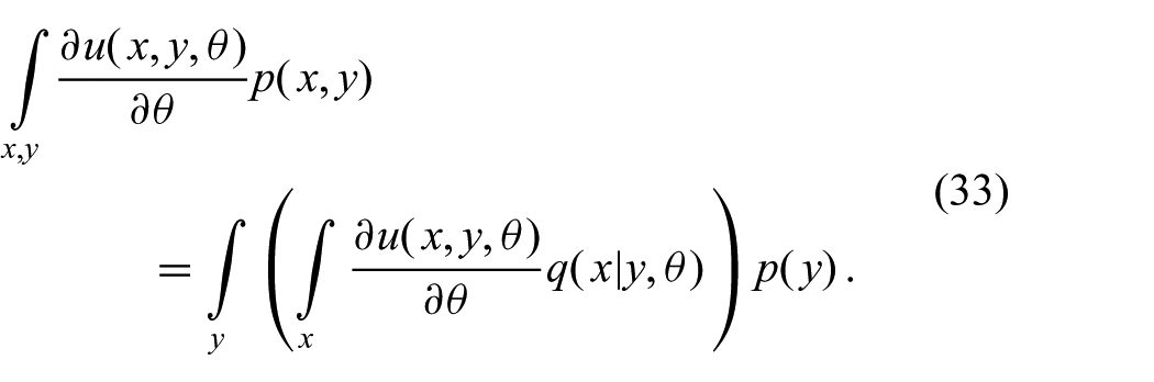
\begin{matrix} \int_{x, y} \frac{\partial u (x, y, θ)}{\partial θ} p (x, y) \\ = \int_{y} (\int_{x} \frac{\partial u (x, y, θ)}{\partial θ} q (x | y, θ)) p (y) . \end{matrix}

(33)

Before this system of equations can be solved, all integrals have to be computed. The integral over x on the right-hand side of (33) is an expectation with respect to the parametric approximation. Since the integrand depends on unknown parameters, this inner integral cannot be approximated numerically. Therefore, $u (\cdot)$ has to be chosen such that there is a closed form solution.

In general, the outer integral over y cannot be solved in closed form since $p (y)$ can have a very complex form, depending on the dynamical system at hand. However, expectations with respect to $p (y)$ can be efficiently approximated numerically, as discussed in Section 3.

Numeric integration is only possible if the integrand depends on no other variable than the ones we integrate out. Therefore, we require $u (\cdot)$ to be such that, after analytically solving the inner integral over x, all the dependences on $θ$ can be moved outside of the integral over y.

On the left-hand side of (33), we evaluate an expectation with respect to $p (x, y)$ . Again, depending on the form of the observation model (2) and the process model (1), it is often not possible to find a closed form solution, but numerical expectations with respect to $p (x, y)$ can be computed efficiently. To allow for numerical integration, $u (\cdot)$ must be such that all the dependences on $θ$ can be moved outside of the integral over x and y.

Finally, after computing the integrals, we have to solve the system of equations (33) in order to find the optimal $θ$ . Therefore, $u (\cdot)$ should be such that this solution can be found efficiently.

It is not clear how the most general $q (x | y, θ)$ complying with the above desiderata can be found. Nevertheless, this discussion can guide the search for more general belief representations than the affine Gaussian that still leave the efficiency of the GF intact. The following section provides an example.

8. The Feature Gaussian Filter

We have seen that any approximate distribution with some required properties can be written in the form of (30). The objective is now to find a function $u (\cdot)$ such that we obtain an efficient filtering algorithm, that is, such that the conditions from Section 7 are satisfied. To obtain some inspiration, we can first find out to which $u (\cdot)$ the family of distributions used in the GF (23b) corresponds. By comparing (30) with (23b), we find

\begin{matrix} u (x, y, A, C) = \\ - \frac{1}{2} {(x - A [\begin{matrix} 1 \\ y \end{matrix}])}^{T} C^{- 1} (x - A [\begin{matrix} 1 \\ y \end{matrix}]) . \end{matrix}

(34)

Next, we generalize this function without violating any of the conditions outlined in Section 7.2. While different ways are conceivable, we propose a straightforward generalization by allowing for nonlinear features in the measurement

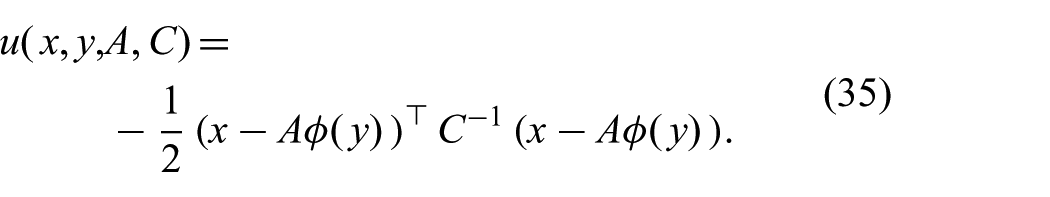
\begin{matrix} u (x, y, A, C) = \\ - \frac{1}{2} {(x - A ϕ (y))}^{T} C^{- 1} (x - A ϕ (y)) . \end{matrix}

(35)

This generalization is mathematically very similar to the generalization of linear regression using features (Bishop, 2006).

Inserting (35) into (30) leads to an approximate distribution which is Gaussian in x, but can have nonlinear dependences on y

q (x | y, A, C) = N (x | A ϕ (y), C) .

(36)

Because this approximation complies with the desiderata from Section 7.2, as we show next, the parameters can be optimized efficiently. We refer to the resulting filtering algorithm as the Feature Gaussian Filter (FGF).

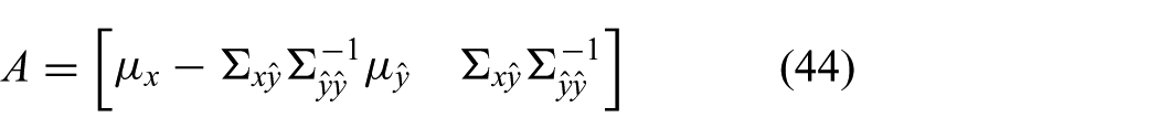
8.1. Solving for A

The derivative of $u (\cdot)$ with respect to A is

\frac{\partial u (x, y, A, C)}{\partial A} = C^{- 1} (x - A ϕ (y)) ϕ (y)^{T} .

(37)

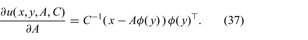
As required, the inner integral in (33) can be solved in closed form since the approximate distribution is Gaussian in x

\int_{x} \frac{\partial u (x, y, A, C)}{\partial A} q (x | y, A, C) = 0 .

(38)

Inserting these results into (33), we can solve for A

A = E [x ϕ (y)^{T}] E [ϕ (y) ϕ (y)^{T}]^{- 1} .

(39)

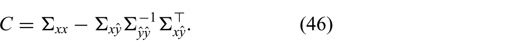
8.2. Solving for C

The matrix C is constrained to be positive definite, such that the approximate distribution (36) is Gaussian. As it turns out, the unconstrained optimization yields a positive definite matrix. Thus, there is no need to take this constraint into account explicitly.

The derivative with respect to $C^{- 1}$ is

\frac{\partial u (x, y, A, C)}{\partial C^{- 1}} = - \frac{1}{2} (x - A ϕ (y)) (x - A ϕ (y))^{T} .

(40)

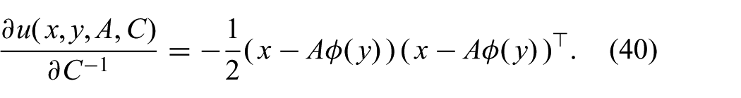
As before, the inner integral in (33) can be solved in closed form since the approximate distribution is Gaussian in x

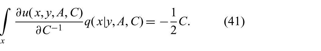
\int_{x} \frac{\partial u (x, y, A, C)}{\partial C^{- 1}} q (x | y, A, C) = - \frac{1}{2} C .

(41)

Inserting these results into (33), we can solve for C

C = E [(x - A ϕ (y)) (x - A ϕ (y))^{T}] .

(42)

8.3. Connection to the Gaussian Filter

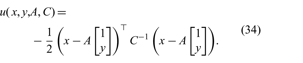
For a feature of the form

ϕ (y) = [\begin{matrix} 1 \\ φ (y) \end{matrix}]

(43)

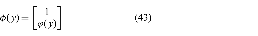
we can see by comparing (35) to (34) that the FGF is equivalent to the GF using a pseudo measurement $\hat{y} = φ (y)$ .

To show how the FGF equations (39) and (42) reduce to the GF equations (17) and (18), we insert $ϕ (y) = [1, {\hat{y}}^{T}]^{T}$ into (39)

A = [\begin{matrix} μ_{x} - Σ_{x \hat{y}} Σ_{\hat{y} \hat{y}}^{- 1} μ_{\hat{y}} & Σ_{x \hat{y}} Σ_{\hat{y} \hat{y}}^{- 1} \end{matrix}]

(44)

with the parameters $μ_{(\cdot)}$ and $Σ_{(\cdot)}$ as defined in (17). The mean of the approximate posterior (36) is now

A ϕ (y) = μ_{x} + Σ_{x \hat{y}} Σ_{\hat{y} \hat{y}}^{- 1} (\hat{y} - μ_{\hat{y}}) .

(45)

Inserting this result into (42), we obtain the covariance

C = Σ_{xx} - Σ_{x \hat{y}} Σ_{\hat{y} \hat{y}}^{- 1} Σ_{x \hat{y}}^{T} .

(46)

Clearly, these equations correspond to the GF equations (18). In particular, with a feature $ϕ (y) = [1, y^{T}]^{T}$ , we retrieve the standard GF.

8.4. Implementation

The FGF could be implemented by computing A as in (39) and C as in (42). In general, the expectations would have to be computed using some numeric integration method, as for the standard GF. Alternatively, an existing implementation of the standard GF can be adapted to implement a FGF with only minor changes.

Implementing a GF requires the specification of a process model (1) and a measurement model (2). The GF’s prediction and update steps are fully determined by those models, and are then applied to the current belief and measurement to compute a new belief at each time step, see Algorithm 1.

Algorithm 1 Gaussian Filter ${g (\cdot), h (\cdot)}$
Require: $p (x_{t - 1} \| y_{1 : t - 1}), y_{t}$
Ensure: $q (x_{t} \| y_{1 : t})$
1: $q (x_{t} \| y_{1 : t - 1}) = predic t_{g} (p (x_{t - 1} \| y_{1 : t - 1}))$
2: $q (x_{t} \| y_{1 : t}) = updat e_{h} (q (x_{t} \| y_{1 : t - 1}), y_{t})$
3: Return $q (x_{t} \| y_{1 : t})$

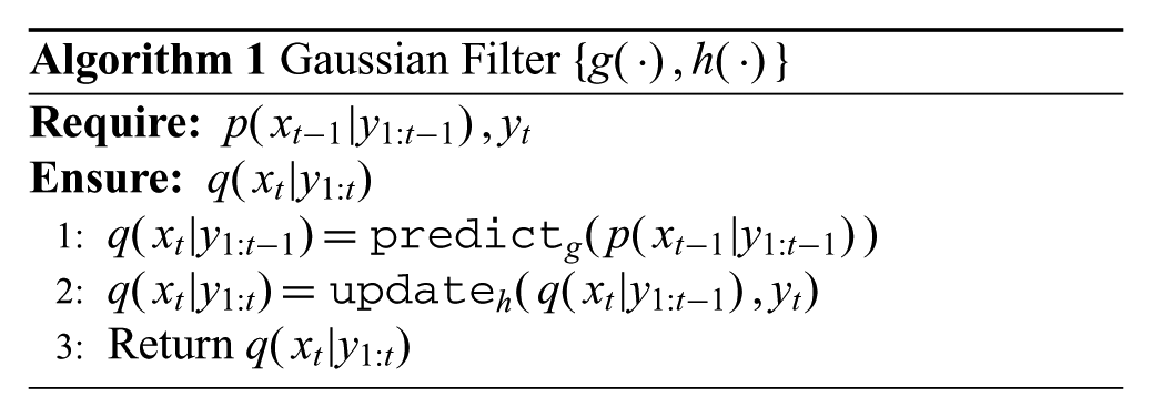
As shown in Section 8.3, the FGF is equivalent to the standard GF using a pseudo measurement $\hat{y} = φ (y)$ , which is obtained by applying a feature function $φ (\cdot)$ to the physical measurement y. The corresponding pseudo measurement model $\hat{h} (x, w) = φ (h (x, w))$ is obtained by composition of the same feature function and the original measurement model. We obtain an FGF from a standard GF by replacing the model $h (\cdot)$ with $\hat{h} (\cdot)$ and the measurements y with $\hat{y}$ , see Algorithm 2. Hence, to implement an FGF, we can simply implement our favorite GF treating $\hat{h} (\cdot)$ as the actual measurement model and $\hat{y}$ as the actual measurement.

Algorithm 2 Feature Gaussian Filter ${g (\cdot), h (\cdot), φ (\cdot)}$
Require: $p (x_{t - 1} \| y_{1 : t - 1}), y_{t}$
Ensure: $q (x_{t} \| y_{1 : t})$
1: $q (x_{t} \| y_{1 : t - 1}) = predic t_{g} (p (x_{t - 1} \| y_{1 : t - 1}))$
2: $\hat{h} (\cdot) = φ (h (\cdot)), {\hat{y}}_{t} = φ (y_{t})$
3: $q (x_{t} \| y_{1 : t}) = updat e_{\hat{h}} (q (x_{t} \| y_{1 : t - 1}), {\hat{y}}_{t})$
4: Return $q (x_{t} \| y_{1 : t})$

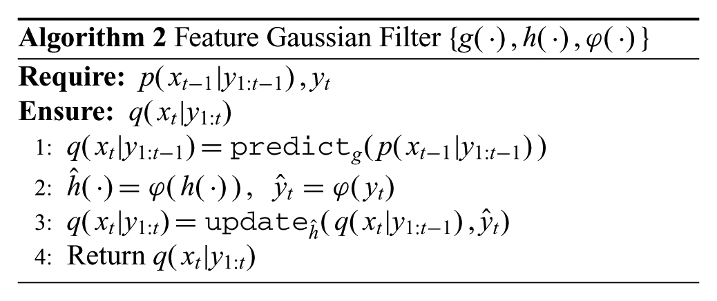
In Section 9, we illustrate how this simple change in implementation can have major effects on the estimation accuracy of the filtering algorithm. We also provide code for a GF that uses Monte Carlo integration and the corresponding FGF.¹

8.5. Related approaches

Applying nonlinear transformations to the physical sensor measurements before feeding them into a GF is not uncommon in robotics and other applications (Daum and Fitzgerald, 1983; Durrant-Whyte, 1996; Rotella et al., 2014; Vaganay et al., 1993). While these transformations are often motivated from physical insight or introduced heuristically, we provide a different interpretation. We see using a measurement feature $φ (y)$ as a means of giving more flexibility to the approximate posterior $q (x | y)$ , which allows it to fit the exact posterior $p (x | y)$ more accurately.

8.6. The more features the better?

The analysis above suggests that adding features will never decrease filtering accuracy.

8.6.1. Redundant features

At first sight, it might be somewhat surprising that there is no problem with using several features containing the same information, that is, which are a function of the same measurement. One might be tempted to think that by doing so, one biases the filter towards this measurement. This is, however, not the case. The more features that are in the feature vector, the more expressive the belief (36) and the better the fit (23a) to the exact posterior $p (x | y)$ . This is mathematically equivalent to using more features in linear regression, where more features always provide a better fit to the data.

To illustrate that the FGF is capable of using redundant features, consider the very simple case of a feature that creates a copy of the measurement

\hat{y} = φ (y) : = [\begin{matrix} y \\ y \end{matrix}] .

(47)

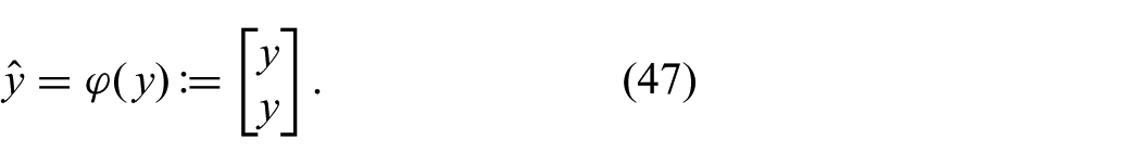
In this case, the FGF will yield precisely the same result as if there were no duplicate of the measurement in the feature.

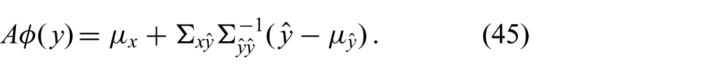
In the following, we perform the FGF calculations by hand to provide some intuition why this happens. The posterior mean is given by (45). As explained in Section 4.1, in an actual implementation, matrix inverses are not computed explicitly. The right-most product of (45) can be written as the solution of the system

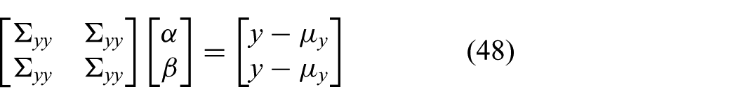
[\begin{matrix} Σ_{yy} & Σ_{yy} \\ Σ_{yy} & Σ_{yy} \end{matrix}] [\begin{matrix} α \\ β \end{matrix}] = [\begin{matrix} y - μ_{y} \\ y - μ_{y} \end{matrix}]

(48)

which yields the constraint

Σ_{yy} (α + β) = y - μ_{y}

(49)

Solving for the FGF mean (45), we obtain

μ_{x} + [\begin{matrix} Σ_{xy} & Σ_{xy} \end{matrix}] [\begin{matrix} α \\ Σ_{yy}^{- 1} (y - μ_{y}) - α \end{matrix}] =

(50)

μ_{x} + Σ_{xy} Σ_{yy}^{- 1} (y - μ_{y})

(51)

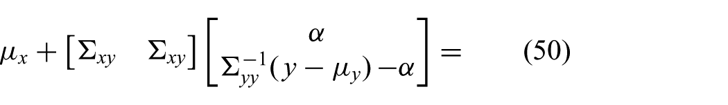
which is the same as we would get with only one copy of the original measurement y. We could reason the same way about the covariance. Hence, adding a copy of a measurement or of a measurement feature does not affect the filtering result. Please note that the above calculation is just for illustration, it will be performed automatically by the filter.

8.6.2. Overfitting

An important question is whether the FGF suffers from overfitting in the same way linear regression suffers from overfitting when too many features are used (Bishop, 2006). In linear regression, the objective is to fit a function to a finite set of points. It is not desirable to fit the points perfectly since this would lead to poor generalization of the function. Here, the situation is fundamentally different. The objective is to fit an approximate distribution $q (x | y)$ to the exact distribution $p (x | y)$ . The more accurately we are able to fit the exact posterior, the better. Hence, there can be no overfitting.

In practice, however, the numeric integration methods in the filter use of course a finite number of samples. Hence, when the number of features is too large with respect to the number of samples used in the numeric integration, then the FGF can suffer from overfitting. Fortunately, we can always generate more samples to offset overfitting, while in linear regression the size of the dataset is fixed.

8.7. Feature selection

There are two ways of selecting features. We can use some generic features in y, such as monomials, without looking at the structure of the problem in detail. If we require even better accuracy, we can hand design a feature for the specific problem at hand. Ideally, one would choose a feature which maps the measurement to a representation which relates to the state linearly.

In Section 9, we give examples of both types of features. We show that the filtering accuracy can be improved significantly by using an appropriate feature.

9. Simulation examples illustrating the benefit of measurement features

As the previous analysis suggests, it is beneficial to augment the measurement with nonlinear features since this gives the approximation more flexibility to fit the exact distribution. In this section, we illustrate this effect in four examples, which are abstractions of relevant filtering problems in robotics. We opt to present small examples to provide insight into specific important aspects of the proposed method, and to give some intuition on how it can be applied to practical filtering problems. A full-scale experimental application is presented in Issac et al. (2016), where a particular type of FGF is used for 3D object tracking using a depth camera.

We implemented the GF using Monte Carlo for the required integrals and the FGF as in Algorithm 2. The code for all the simulations is publicly available, see endnote 1. In the two first examples, it is possible to solve the integrals analytically, so we present here the exact results rather than the approximate ones.

The first two examples use monomials as features and illustrate why using such features can have a major impact on the estimation accuracy. The last two examples illustrate how features can be designed for specific systems. Another example of a designed feature is given in Wüthrich et al. (2016), where the authors derive a feature in order to handle fat-tailed measurement models.

9.1. Estimation of sensor noise magnitude

The measurement process (2) of a dynamical system can often be represented by a nonlinear observation model with additive noise

h (x, M, w) = \tilde{h} (x) + Mw

(52)

where $\tilde{h}$ is a nonlinear function of the system state, and the matrix M determines the magnitude of the sensor noise (recall that w is Gaussian with zero mean and unit variance). Often, the sensor standard deviation (i.e. the matrix M) is not precisely known, or it may be time varying due to changing sensor properties and environmental conditions. It is then desirable to estimate the noise matrix M alongside the state x. In the following, we show that this is not possible with the standard GF, but can be achieved with the FGF.

We define an augmented state $\hat{x} : = (x; m)$ , where m is a column vector containing all the elements of the noise matrix M. The observation model in distributional form is $p (y | \hat{x}) = p (y | x, m) = N (y | \tilde{h} (x), M M^{T})$ . The state x and the parameters m stem from independent processes, and we therefore have $p (\hat{x}) = p (x) p (m)$ . Let us now apply the standard GF to this problem by computing the parameters in (17). In particular, we compute the covariance between the augmented state and the measurement

\begin{matrix} Σ_{\hat{x} y} = \\ \int_{x, m, y} [\begin{matrix} x - μ_{x} \\ m - μ_{m} \end{matrix}] {(y - μ_{y})}^{T} p (y | x, m) p (x) p (m) . \end{matrix}

(53)

The integral over y can be solved easily since $p (y | x, m)$ is Gaussian

Σ_{\hat{x} y} = \int_{x, m} [\begin{matrix} x - μ_{x} \\ m - μ_{m} \end{matrix}] (\tilde{h} (x) - μ_{y})^{T} p (x) p (m) .

(54)

Interestingly, the second factor does not depend on m. Therefore, the integral over m is solved easily and yields

Σ_{\hat{x} y} = \int_{x} [\begin{matrix} x - μ_{x} \\ μ_{m} - μ_{m} \end{matrix}] (\tilde{h} (x) - μ_{y})^{T} p (x)

(55a)

= [\begin{matrix} Σ_{xy} \\ 0 \end{matrix}]

(55b)

As a result, there is no linear correlation between the measurement y and the parameters m. Inserting this result into (18) shows that the innovation corresponding to m is zero. The corresponding part of the covariance matrix does not change either. Hence, the measurement has no effect on the estimate of m. It will behave as if no observation had been made. This illustrates the failure of the GF to capture certain dependences in nonlinear dynamical systems.

In contrast, if a nonlinear feature in the measurement y is used, the integral over y in (53) will not yield $\tilde{h} (x)$ , but instead some function depending on both x and m. This dependence allows the FGF to infer the desired parameters, as is shown next.

In the remainder of the paper, we are considering several time steps again, and will thus reintroduce the time indices, which we dropped earlier.

9.1.1. Numerical example

For the purpose of illustrating the theoretical argument above, we use a small toy example. We consider a single sensor, where all quantities in (52), including the standard deviation $M_{t}$ , are scalars. Since we are only interested in the estimate of $M_{t}$ , we choose $\tilde{h} (x_{t}) = 0$ . The observation model (52) simplifies to

y_{t} = h (M_{t}, w_{t}) = M_{t} w_{t} .

(56)

Choosing a simple process model

M_{t} = g (M_{t - 1}, v_{t}) = M_{t - 1} + 0.1 v_{t}

(57)

the dynamical system (1), (2) is fully defined. Recall that we defined the noise $v_{t}$ and $w_{t}$ to be drawn from Gaussians with zero mean and unit variance.

This example captures the fundamental properties of the FGF as pertaining to the estimation of sensor noise intensity $M_{t}$ . The same qualitative effects hold for multivariate systems (52) for the reasons stated above.

In Figure 3, we show the simulation result of a single update step. The true density in grayscale was computed numerically for the purpose of comparison. It would, of course, be too expensive to use in a filtering algorithm.

Fig. 3.

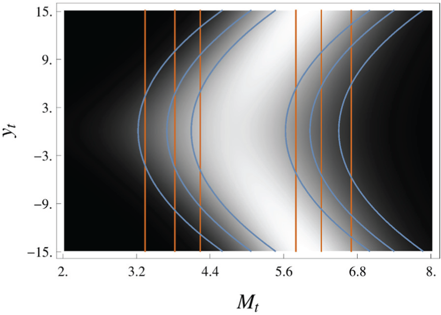
Simulation of a single update step with prior $p (M_{t}) = N (M_{t} | 5, 1)$ , and observation model (56). The density (white for large values) represents the true posterior $p (M_{t} | y_{t})$ . The overlaid contour lines show the approximate posterior $q (M_{t} | y_{t})$ of the GF in orange and of the FGF in blue.

The overlaid orange contour lines show the approximate conditional distribution $q (M_{t} | y_{t})$ obtained with the standard GF. No matter what measurement $y_{t}$ is obtained, the posterior $q (M_{t} | y_{t})$ is the same. The GF does not react to the measurements at all.

The true conditional distribution $p (M_{t} | y_{t})$ depends on $y_{t}$ , which means that the measurement does in fact contain information about the state $M_{t}$ . However, the approximation $q (M_{t} | y_{t})$ made by the GF is not expressive enough to capture this information, which results in a very poor fit to $p (M_{t} | y_{t})$ .

As explained in Section 8.3, the standard GF is the special case of the FGF with the feature $ϕ (y_{t}) = [1, y_{t}]^{T}$ . Let us take the obvious next step and add a quadratic term to the feature $ϕ (y_{t}) = [1, y_{t}, y_{t}^{2}]^{T}$ . The resulting approximation is represented by the blue contour lines in Figure 3. Clearly, $q (x_{t} | y_{t})$ now depends on the measurement $y_{t}$ , which allows the FGF to exploit the information about the state $x_{t}$ contained in the measurement. The approximation $q (x_{t} | y_{t})$ of the FGF has a more flexible form, which allows for a better fit of the true posterior.

To analyze actual filtering performance, we simulate the dynamical system and the two filters for 1000 time steps. The results are shown in Figure 4.

Fig. 4.

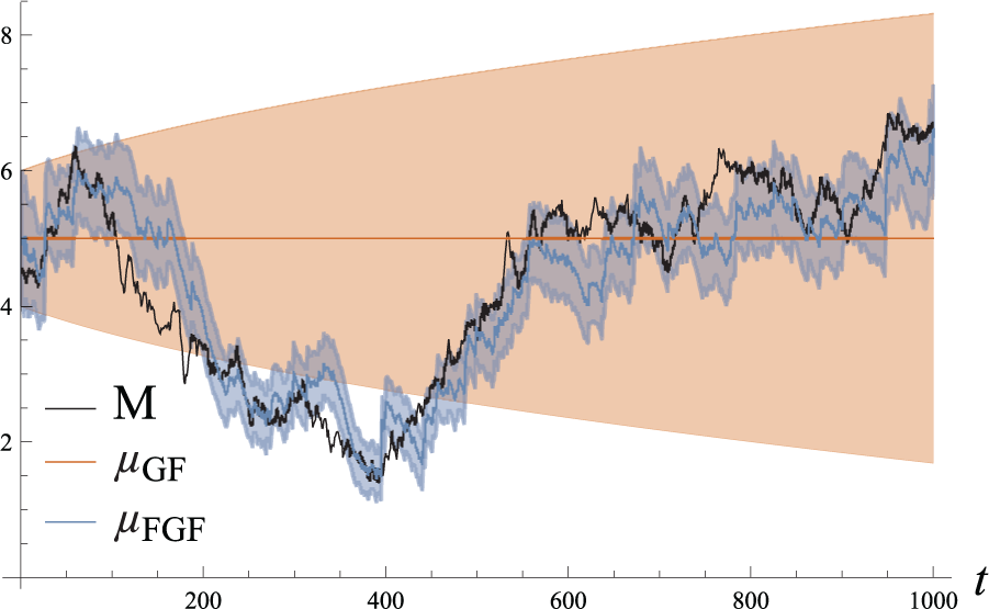
Simulation of the system (56), (57) for 1000 time steps. The simulated noise parameter $M_{t}$ is shown in black, together with the mean and standard deviation of the estimates obtained with the GF (orange) and the FGF (blue).

As expected, the standard GF does not react in any way to the incoming measurements. The FGF, on the other hand, is capable of inferring the state $M_{t}$ from the measurements $y_{t}$ , as suggested by the theoretical analysis above.

9.1.2. Insights

While it was convenient to simulate a very simple system for illustration purposes, it is important to note that the theoretical argument given above applies to realistic, nonlinear and multivariate systems. We showed that it is not possible to infer the sensor noise magnitude using a standard GF, a problem which can be solved by using a nonlinear measurement feature. This result could be useful for any filtering problem where the sensor accuracy is not precisely known or varies over time.

9.2. Nonlinear observation model

In this section, we investigate how the theoretical benefit of adding nonlinear features translates into improved filtering performance for systems with nonlinear observation models. To clearly illustrate the difference of GF and FGF, we choose a simple system with a strong nonlinearity (step function).

The process model and the observation model are given by

x_{t} = g (x_{t - 1}, v_{t}) = x_{t - 1} + v_{t}

(58)

y_{t} = h (x_{t}, w_{t}) = x_{t} + w_{t} + 50 H (x_{t})

(59)

where $H (\cdot)$ is the Heaviside step function.

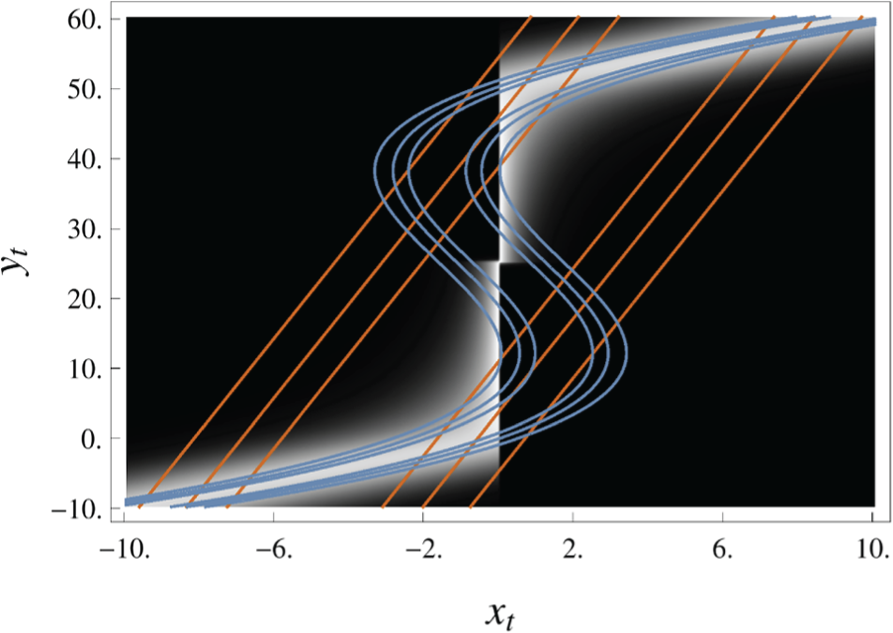
In Figure 5, we plot the true conditional density $p (x_{t} | y_{t})$ with overlaid orange contour lines of the approximate conditional distribution $q (x_{t} | y_{t})$ obtained using the standard GF.

Fig. 5.

Simulation of a single update step with prior $p (x_{t}) = N (x_{t} | 0, 5)$ , and observation model (59). The density (white for large values) represents the true posterior $p (x_{t} | y_{t})$ . The overlaid contour lines show the approximate posterior $q (x_{t} | y_{t})$ of the GF in orange and of the FGF in blue.

The contour lines reflect the restrictions on the posterior of the GF (23b). The mean of the approximate density $q (x_{t} | y_{t})$ is an affine function of the measurement $y_{t}$ . For nonlinear observation models, this coarse approximation can lead to the loss of valuable information contained in the measurement $y_{t}$ .

The approximate density $q (x_{t} | y_{t})$ obtained using a feature $ϕ (y_{t}) = [1, y_{t}, y_{t}^{2}, y_{t}^{3}]^{T}$ , which is represented by the blue contour lines in Figure 5, fits the true posterior much better. This illustrates that nonlinear features allow for approximate posteriors with much more elaborate dependences on $y_{t}$ .

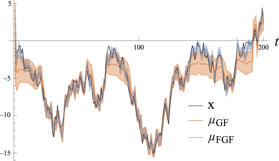
Figure 6 shows how this difference translates to filtering performance. When $x_{t}$ is far away from zero, the nonlinearity has no effect; the system behaves like a linear system. The density plot in this regime would be centered at a linear part of the distribution, and both filters would achieve a perfect fit. Both the standard GF and the FGF are therefore optimal in that case. When the state is close to zero, however, the advantage of the FGF becomes apparent. Its tracking performance is good even when the state is close to the nonlinearity of the observation model, due to more flexibility in $y_{t}$ of the posterior approximation $q (x_{t} | y_{t})$ .

Fig. 6.

Simulation of the system (58), (59) for 200 time steps. The simulated state $x_{t}$ is shown in black, together with the mean and standard deviation of the estimates obtained with the GF (orange) and the FGF (blue).

9.2.1. Insights

This simulation shows that using a measurement feature can greatly improve filtering performance. Based on the theoretical analysis and this example, we believe that it is plausible that using measurement features can also significantly improve accuracy for systems with more realistic nonlinearities.

9.3. Measurement in polar coordinates

Suppose we want to estimate the two-dimensional position $x_{t}$ of an object, using distance $r_{t}$ and the bearing $γ_{t}$ measurements, see Figure 7.

Fig. 7.

We want to estimate the state $x_{t} = [x_{t}^{[1]}, x_{t}^{[2]}]^{T}$ using range $r_{t}$ and bearing $γ_{t}$ measurements.

Such measurements are for example generated by sonar and radar sensors (Durrant-Whyte, 1996; Julier and Uhlmann, 1997; Karlgaard and Schaub, 2006).

We define the process model to be linear Gaussian in Cartesian coordinates

x_{t} = g (x_{t - 1}, v_{t}) = x_{t - 1} + v_{t}

(60)

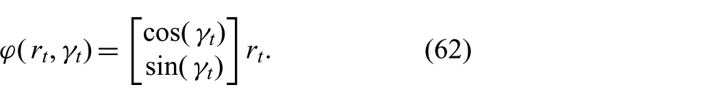
and the observation model is given by

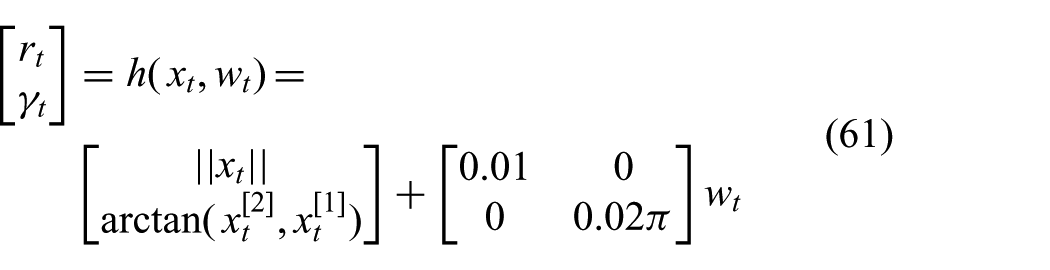
\begin{matrix} [\begin{matrix} r_{t} \\ γ_{t} \end{matrix}] = h (x_{t}, w_{t}) = \\ [\begin{matrix} | | x_{t} | | \\ \arctan (x_{t}^{[2]}, x_{t}^{[1]}) \end{matrix}] + [\begin{matrix} 0.01 & 0 \\ 0 & 0.02 π \end{matrix}] w_{t} \end{matrix}

(61)

where the superscripts index the vector elements. The nonlinear function applied to $x_{t}$ is the coordinate transformation from Cartesian to polar coordinates. The standard deviation of the process model is about two orders of magnitude larger than the one of the sensor. Such a configuration can occur for instance when we dispose of a sensor which is accurate, but provides measurements at a low rate. During the large time difference between two measurements, the object might move quite far, which implies a large standard deviation in the process model.

It is not uncommon in the filtering literature to transform measurements of this type back to Cartesian coordinates before filtering, see, for example, Durrant-Whyte (1996). This corresponds to using the measurement feature

φ (r_{t}, γ_{t}) = [\begin{matrix} \cos (γ_{t}) \\ \sin (γ_{t}) \end{matrix}] r_{t} .

(62)

Intuitively, this makes the task of the filter easier since the relation between the transformed measurement and the state is simpler. We show that this technique can indeed improve performance significantly for parts of the state space by allowing the approximate posterior to fit the exact posterior more accurately.

Furthermore, the analysis in this paper suggests that it is not necessary to choose between one measurement representation or the other. We can simply stack both of them, and the filter will automatically weight them.

Figure 8 shows that using the measurement feature (62) (we refer to this filter as Cartesian-FGF) can significantly improve filtering accuracy. The gain in accuracy is the greatest when the object is close to zero in at least one of the axes. This is because the measurement function (61) is highly nonlinear in this area.

Fig. 8.

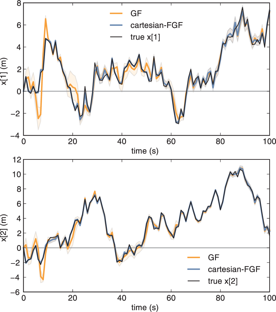
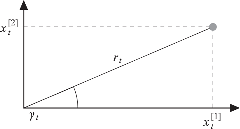
Simulation of the system (60), (61) for 100 time steps. The simulated state $x_{t}$ is shown in black, together with the mean and standard deviation of the estimates obtained with the GF (orange) and the cartesian-FGF (blue).

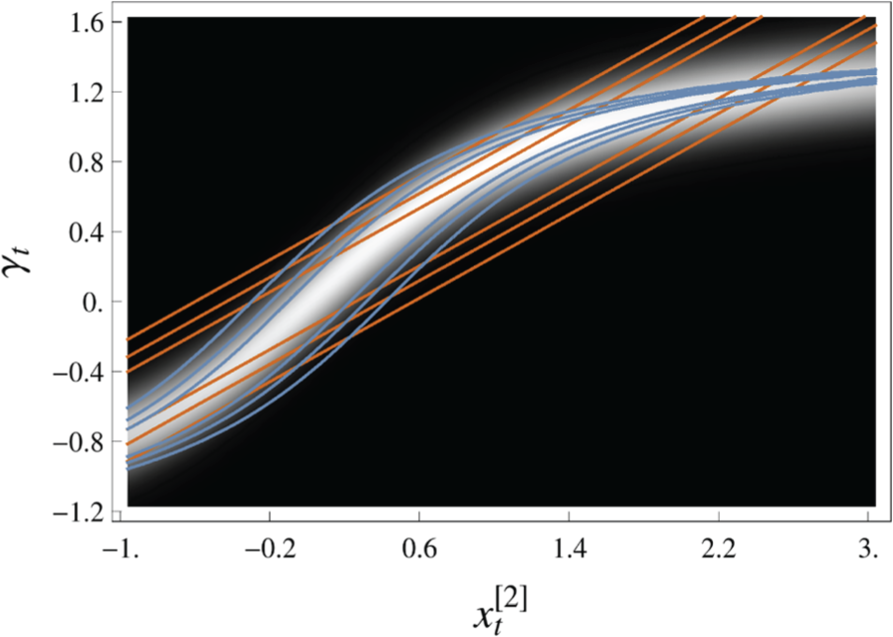
To understand this difference in estimation accuracy, we show the relationship between the state dimension $x_{t}^{[2]}$ and the angle $γ_{t}$ in Figure 9. The fit obtained using the standard GF is suboptimal due to the nonlinearity of the coordinate transformation in the observation model (61). This nonlinearity can be partly canceled by using the feature (62), which allows the Cartesian-FGF to fit the posterior more accurately. It is important to note that it is not possible to cancel the nonlinearity in (61) perfectly, because the noise is added in polar coordinates. For small noise variance however, we can expect the cancellation to work well.

Fig. 9.

A visualization of the dependence between $x_{t}^{[2]}$ and $γ_{t}$ in a single update step. The first state dimension $x_{t}^{[1]} = 1$ is fixed, and the prior is $p (x_{t}^{[2]}) = N (x_{t}^{[2]} | 1, 1)$ . The density plot (white for large values) represents the true posterior $p (x_{t}^{[2]} | γ_{t})$ with overlaid contour lines of the approximate conditional distribution $q (x_{t}^{[2]} | γ_{t})$ of the GF (orange) and the Cartesian-FGF (blue).

9.3.1. Insights

We have shown that using the measurement feature (62) can improve the estimation accuracy when the object is close to zero. However, when the object is further away from zero, the improvement vanishes. More generally, the benefits of a particular feature depend on the parameters of the problem at hand, and on the state the system is currently in. While using a particular feature might improve estimation accuracy for one particular configuration, it could potentially worsen accuracy in a different configuration. Hence, the question arises which feature mapping should be used for a particular problem.

Fortunately, we can just stack all the features and the original measurements, and the filter will weight them automatically. The filter will autonomously pick the features which allow it to best represent the posterior belief in the particular configuration it is in. As discussed in Section 8.6.2, as long as the numeric integration method is accurate enough, there will be no overfitting.

We illustrate this effect in Figure 10, where we compare the Cartesian-FGF to an FGF using monomials as features. We see that using monomials of degree 2 only seems to improve the filtering accuracy slightly. In this case, the best measurement representation is clearly (62). The filter which combines all features and the original measurement (all-FGF) performs equally well since it automatically picks the best representation.

Fig. 10.

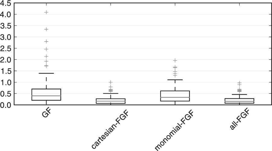
The boxplots represent the distribution of the tracking error. Each data point is the error at one time step of the simulation of the system (60), (61). The GF uses the plain observation $[r_{t}, γ_{t}]^{T}$ , the cartesian-FGF uses the feature (62), the monomial-FGF uses monomials of degree 2 and the all-FGF uses a feature vector combining all these features.

9.4. 2-link planar robot

In this simulation, we look at the problem of estimating the joint angles of a robot given information about the end-effector pose. This problem is practically relevant, because the joint readings can be unreliable due to noisy sensors, drift, cable stretch or poor calibration. We therefore seek to obtain a more accurate estimate of the joint angles by incorporating a sensor which yields measurements of the end-effector pose. This sensor might be a camera on the robot, which performs simultaneous localization and mapping (SLAM); it might be an external camera, which detects the position of the end-effector, or it could be an inertial measurement unit (IMU), which is mounted on the end-effector. For instance, we might want to estimate the configuration of the neck of a humanoid robot using the joint sensors as well as the head-mounted camera.

The relation between end-effector pose and joint angles is highly nonlinear, which means that the GF is not able to exploit all the available information. To illustrate this problem, we simulate the two-link robot in Figure 11. The state $x_{t}$ consists of the joint angles, and the transition model is linear Gaussian

x_{t} = g (x_{t - 1}, v_{t}) = x_{t - 1} + 0.1 π v_{t} .

(63)

We receive noisy measurements of the joint angles

[\begin{matrix} y_{t}^{[1]} \\ y_{t}^{[2]} \end{matrix}] = x_{t} + 0.2 π [\begin{matrix} w_{t}^{[1]} \\ w_{t}^{[2]} \end{matrix}]

(64)

and relatively accurate measurements of the end-effector position

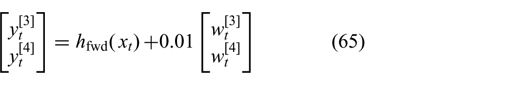
[\begin{matrix} y_{t}^{[3]} \\ y_{t}^{[4]} \end{matrix}] = h_{f wd} (x_{t}) + 0.01 [\begin{matrix} w_{t}^{[3]} \\ w_{t}^{[4]} \end{matrix}]

(65)

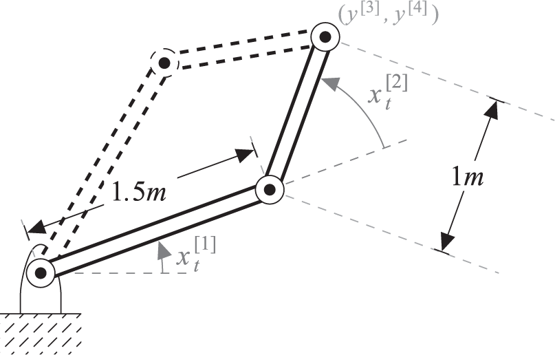
where $h_{f wd}$ are the forward kinematics of the robot.

Fig. 11.

Kinematics of a two link manipulator. The state $x_{t} = (x_{t}^{[1]}, x_{t}^{[2]})$ consists of the joint angles and the measurement $y_{t}$ of the end-effector position.

An obvious candidate for a feature is the inverse kinematics. There are however two solutions, as shown in Figure 11. We will denote the solution with the elbow on the left side by $in v_{l} (\cdot)$ and the solution with the elbow on the right side by $in v_{r} (\cdot)$ . We could apply either of these two as features to the position measurements.

In Figure 12, we show the filtering performance using the two features. Not surprisingly, the filter using $in v_{l} (\cdot)$ as the feature (green) performs well as long as the robot actually has its elbow bent towards the left side. However, when the robot switches to the right sided configuration at around $60 s$ , this feature does not yield good estimates anymore, and the filter using $in v_{r} (\cdot)$ (orange) starts performing well. Fortunately, we can simply filter using both features, which yields good performance everywhere (blue). The filter automatically assigns more weight to the feature $in v_{r} (\cdot)$ when the robot is in a configuration where the elbow is pointing to the left, because it allows the exact posterior to be fitted accurately. Conversely, the filter will automatically use the feature $in v_{r} (\cdot)$ to fit the exact posterior well when the elbow is pointing towards the right.

Fig. 12.

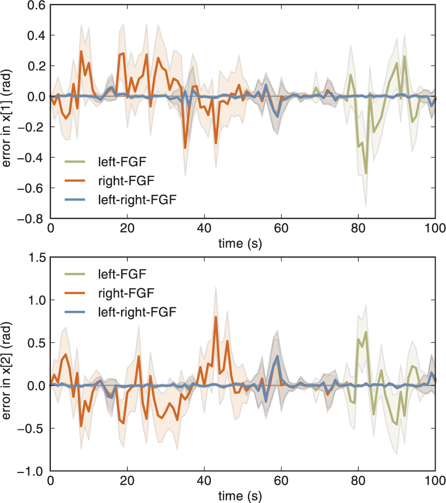
Simulation of the system (63), (64), (65) for 100 time steps. We plot the mean errors and standard deviations of the estimates obtained using $in v_{l} (\cdot)$ as feature (orange), using $in v_{r} (\cdot)$ as feature (green) and using both features (blue).

In Figure 13, we compare the estimation accuracy using different features. In this example, using monomials of degree 2 already improves estimation accuracy significantly. A further improvement can be obtained using the problem-specific features, that is, the inverse kinematics. As in the previous example, using all features at once yields an estimation accuracy which is at least as good as the filters using the individual features.

Fig. 13.

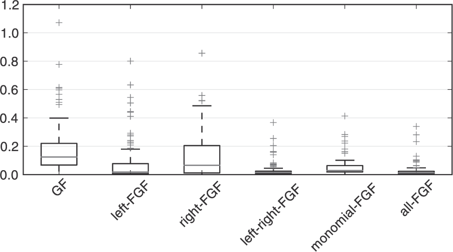
The boxplots represent the distribution of the tracking error. Each data point is the error at one time step of the simulation of the system (63), (64), (65). The GF uses the plain observation $y_{t}$ , the left-FGF uses $in v_{l} (\cdot)$ , the right-FGF uses $in v_{r} (\cdot)$ , the left-right-FGF uses both $in v_{l} (\cdot)$ and $in v_{r} (\cdot)$ and the monomial-FGF uses monomials of degree 2 as features. Finally, the all-FGF combines all of the above features.

9.4.1. Insights

This example provides some intuition into how the insights from this paper can be applied to larger, more realistic problems. It shows that using generic measurement features, here monomials, can improve estimation accuracy significantly. By using problem-specific features which approximately cancel the nonlinearity in the observation model, we can typically further improve accuracy. This example also shows that it is possible to combine different features which are complementary. The filter will automatically assign weight to the features necessary for approximating the exact posterior well.

10. Discussion

The key insight in this article is that the GF can be understood as the solution to a constrained optimization problem. From this new perspective, the GF is seen as a special case of a much broader class of filters obtained by relaxing the constraint on the form of the approximate posterior.

On this basis, we outlined some conditions which potential generalizations have to satisfy in order to maintain the properties which make the GF computationally efficient.

We proposed one particular, straightforward generalization which corresponds to filtering with a pseudo measurement. Extending an existing GF implementation in this manner is trivial. Nevertheless, we showed that this small change can have a major impact on the estimation accuracy.

The simulations provided in this article are abstractions of realistic problems, they serve to illustrate the theoretical concepts and to provide intuition on how these could be applied to practical filtering problems. The ideas in this paper are not intended to solve one concrete filtering problem, but rather to provide a theoretical basis for future research. In fact, these insights have already given rise to practical filtering algorithms in Wüthrich et al. (2016) and Issac et al. (2016). The first reference proposes using a measurement feature for robustifying GFs against outliers. The second one applies this idea to 3D object tracking using a depth sensor, which provides measurements contaminated with outliers.

10.1. Directions

One interesting direction of future work is to attempt to further relax the constraint on the form of the approximation, without violating the conditions which ensure computational efficiency. For instance, could we allow for an approximate belief where not just the mean, but also the covariance depends on the measurement?

Explicitly taking the inaccuracy of the numerical integration method into account is another interesting direction for future work. Doing so would be necessary to guarantee that our belief in fact approximates the exact posterior well, even when the numeric approximation is not perfect. An analysis based on learning theory (Vapnik, 1995) might make sense. We would expect a trade-off between the number of samples in the numeric integration and the complexity of the form of the belief. For the FGF, this would mean that the more samples we use in the numeric integration, the more features we can use simultaneously without overfitting.

Footnotes

Appendix 1. Posterior mean and covariance as solutions of a linear system

Recall the GF posterior

\begin{matrix} q (x | y) = \\ N (x | \underset{μ_{x | y}}{\underset{︸}{μ_{x} + Σ_{xy} Σ_{yy}^{- 1} (y - μ_{y})}}, \underset{Σ_{xx | y}}{\underset{︸}{Σ_{xx} - Σ_{xy} Σ_{yy}^{- 1} Σ_{xy}^{T}}}) . \end{matrix}

(18 revisited)

The posterior mean can be formulated as the solution of the linear system

(66a)

μ_{x | y} = μ_{x} + \sum_{xy} a

(66b)

\sum_{yy} a = y - μ y

(66c)

variables : μ_{x | y}, a

where we have introduced an auxiliary vector a of the same size as y. Similarly, we can find the posterior covariance by solving

(67a)

\sum_{xx | y} = \sum_{xx} - \sum_{xy} A

(67b)

\sum_{yy} A = \sum_{xy}^{T}

(67c)

variable : \sum_{xx | y}, A

where we have introduced the auxiliary matrix A of appropriate dimensions.

These systems can be passed to any linear solver, since there exists a unique solution for $μ_{x | y}$ and $Σ_{xx | y}$ , even when $Σ_{yy}$ is degenerate, as we will prove in the following.

Declaration of conflicting interests

The authors declare that there is no conflict of interest.

Funding

This research was supported in part by the Max Planck ETH Center for Learning Systems, the Max Planck Society, National Science Foundation grants IIS-1205249, IIS-1017134, EECS-0926052, the Office of Naval Research and the Okawa Foundation. Any opinions, findings, and conclusions or recommendations expressed in this material are those of the authors and do not necessarily reflect the views of the funding organizations.

Notes

References

Anderson

BDO

Moore

(1979) Optimal Filtering. Englewood Cliffs, NJ: Prentice-Hall.

Arasaratnam

Haykin

(2009) Cubature Kalman filters. IEEE Transactions on Automatic Control 54(6): 1254–1269.

Barber

(2012) Bayesian Reasoning and Machine Learning. New York: Cambridge University Press.

Beneš

(1981) Exact finite-dimensional filters for certain diffusions with nonlinear drift. Stochastics 5(1-2): 65–92.

Bickel

Bengtsson

(2008) Sharp Failure Rates for the Bootstrap Particle Filter in High Dimensions (Collections, vol. 3). Beachwood, OH: Institute of Mathematical Statistics, pp.318–329.

Bishop

(2006) Pattern Recognition and Machine Learning (Information Science and Statistics). Secaucus, NJ: Springer-Verlag New York, Inc.

Cappé

Godsill

Moulines

(2007) An overview of existing methods and recent advances in sequential Monte Carlo. Proceedings of the IEEE 95(5): 899–924.

Daum

(1986) Exact finite-dimensional nonlinear filters. IEEE Transactions on Automatic Control 31(7): 616–622.

Daum

Fitzgerald

(1983) Decoupled Kalman filters for phased array radar tracking. IEEE Transactions on Automatic Control 28(3): 269–283.

10.

Durrant-Whyte

(1996) An autonomous guided vehicle for cargo handling applications. International Journal of Robotics Research 15(5): 407–440.

11.

Gordon

Salmond

Smith

AFM

(1993) Novel approach to nonlinear/non-Gaussian Bayesian state estimation. IEE Proceedings F (Radar and Signal Processing) 140(2): 107–113.

12.

Issac

Wüthrich

Garcia Cifuentes

. (2016) Depth-Based Object Tracking Using a Robust Gaussian Filter. In: Okamura

(ed.) Robotics and automation (ICRA), IEEE international conference on, Stockholm, 16–21 May 2016, pp.608–615. New York: IEEE.

13.

Ito

Xiong

(2000) Gaussian filters for nonlinear filtering problems. IEEE Transactions on Automatic Control 45(5): 910–927.

14.

Julier

Uhlmann

(1997) A new extension of the Kalman filter to nonlinear systems. In:Proceedings of AeroSense: The 11th int. symp. on aerospace/defense sensing, simulations and controls, pp.182–193. Bellingham, Washington, USA: International Society for Optics and Photonics.

15.

Kalman

(1960) A new approach to linear filtering and prediction problems. Transactions of the ASME - Journal of Basic Engineering (82 (Series D)): 35–45.

16.

Karlgaard

Schaub

(2006) Comparison of several nonlinear filters for a benchmark tracking problem. In: AIAA guidance, navigation, and control conference and exhibit, Keystone, CO, 21–24 August 2006. Reston, Virgina: American Institute of Aeronautics and Astronautics.

17.

Kushner

(1967) Approximations to optimal nonlinear filters. IEEE Transactions on Automatic Control 12(5): 546–556.

18.

Kushner

Budhiraja

(2000) A nonlinear filtering algorithm based on an approximation of the conditional distribution. IEEE Transactions on Automatic Control 45(3): 580–585.

19.

Bengtsson

Bickel

(2005) Curse-of-dimensionality revisited: Collapse of importance sampling in very large scale systems. Technical report, Department of Statistics, UC-Berkeley.

20.

MacKay

(2003) Information Theory, Inference and Learning Algorithms. Cambridge: Cambridge University Press.

21.

Maybeck

(1979) Stochastic Models, Estimation and Control (Mathematics in Science and Engineering). Cambridge, Massachusetts, USA: Academic Press.

22.

Minka

(2001) Expectation propagation for approximate Bayesian inference. In: Proceedings of the 17th conference in uncertainty in artificial intelligence, Seattle, Washington, USA, 2–5 August 2001, pp.362–369. Burlington, Massachusetts: Morgan Kaufmann Publishers.

23.

Morelande

Garcia-Fernandez

(2013) Analysis of Kalman filter approximations for nonlinear measurements. IEEE Transactions on Signal Processing 61(22): 5477–5484.

24.

Murphy

(2012) Machine Learning: A Probabilistic Perspective. Cambridge, MA: The MIT Press.

25.

Nørgaard

Poulsen

Ravn

(2000) New developments in state estimation for nonlinear systems. Automatica 36(11): 1627–1638.

26.

Owen

(2013) Monte Carlo theory, methods and examples (book draft). Available at: http://statweb.stanford.edu/owen/mc/ (accessed 1 January 2016).

27.

Rotella

Bloesch

Righetti

. (2014) State estimation for a humanoid robot. In: IEEE/RSJ international conference on intelligent robots and systems, Hong Kong, 31 May–7 June 2014, pp.952–958. New York: IEEE.

28.

Särkkä

(2013) Bayesian Filtering and Smoothing. New York: Cambridge University Press.

29.

Sorenson

(1960) Kalman Filtering: Theory and Application. New York: IEEE Press.

30.

Vaganay

Aldon

Fournier

(1993) Mobile robot attitude estimation by fusion of inertial data. In: IEEE international conference on robotics and automation, volume 1, Atlanta, Georgia, USA, 2–6 May 1993, pp.277–282. New York: IEEE.

31.

van der Merwe

Wan

(2003) Sigma-Point Kalman Filters for probabilistic inference in dynamic state-space models. In: In proceedings of the workshop on advances in machine learning, Montreal, Canada, 8–11 June 2003.

32.

Vapnik

(1995) The Nature of Statistical Learning Theory. Springer-Verlag New York, Inc.

33.

. (2006) A numerical-integration perspective on Gaussian filters. IEEE Transactions on Signal Processing 54(8): 2910–2921.

34.

Wüthrich

Garcia Cifuentes

Trimpe

. (2016) Robust Gaussian Filtering using a Pseudo Measurement. In: Proceedings of the American control conference, Boston, USA, 6–8 July 2016, pp.3606–3613. New York: IEEE.

35.

Wüthrich

Trimpe

Kappler

. (2015) A new perspective and extension of the Gaussian Filter. In: Robotics: Science and systems (R:SS), Rome, Italy, 13–17 July 2015. RSS foundation.