3D kinematic modeling of a self-reconfigurable wheeled mobile robot for enhancing multimode motion capability

Abstract

Self-reconfigurable wheeled mobile robots (SRWMRs) are capable of achieving multiple motion modes and subsequent switching between them through the coordinated sequential movements of multiple rocker–bogie joints, leading to overcoming dynamic obstacles posed by different terrains. However, real-time coordination of internal joints for executing reconfiguration actions while maintaining strong adhesion between the wheels and terrain remains challenging, particularly during action transitions. To enhance multimode motion capability by using a unified model, this work develops an inverse kinematics control (IKC) method, including 3D kinematic modeling of an SRWMR with actively and passively articulated suspensions, and additional motion-constraint inequalities for multi-joints in the wheel-suspension system. Specifically, the 3D model is built to achieve horizontal movements and vertical lifting of the robot chassis and its wheels. To further stabilize body posture and reduce wheel slippage during multimode motion, motion constraints are proposed to regulate the relative velocities among multiple joints and the displacement of the robot’s center of mass. According to the results of physical experiments with the HIT-MRII robot, Wheel Rolling, Wheel Crabbing, Wheel Lifting, Robot Chassis Lifting, Robot Creeping modes, and parts of their hybrid modes are achieved steadily and safely by the developed IKC method. The maximum motion performance of each mode is achieved by the proposed motion constraints. The enhanced mobility of the robot is demonstrated by comparing various traversal modes on soil terrain and presenting the corresponding control strategies.

Keywords

self-reconfigurable wheeled mobile robots multimode motion control 3D kinematic model motion constraint

1. Introduction

Self-reconfigurable wheeled mobile robots (SRWMRs), possessing multimode motion capabilities, are increasingly significant in traversing irregular obstacles on unknown terrains, especially on extraterrestrial surfaces such as the Moon and Mars (Moubarak and Ben-Tzvi, 2012). To enable path-following locomotion in the wheeled mobile robot (WMR) equipped with passive suspension systems, the inverse kinematics control plays a crucial role in establishing the fundamental velocity transmission from the body to its wheels (Toupet et al., 2020). However, the inclusion of reconfiguration actions in the kinematic model, particularly for the SRWMR equipped with both actively and passively articulated suspensions, poses a significant model-building challenge. This results from the multiple degrees of freedom in the vertical velocities for both the robot body and its wheels. Consequently, an efficient three-dimensional (3D) kinematic model for the SRWMR is required to enable both horizontal locomotion and vertical reconfiguration. In addition, the synchronized control of varying wheel velocities and the sequential actions of rocker–bogie mechanisms significantly increase the complexity of maintaining stable robot posture. To ensure reconfiguration functionality and posture stability, the relative positions and velocities of the robot rocker–bogies and its wheels need to be taken into account as additional constraints on the basis of the 3D inverse kinematics control.

The control design of multimode motion in an SRWMR is crucial for enhancing mobility across diverse terrains with complex obstacles. Recent attention has been directed toward studies of WMRs with active-rocker arms. A notable example is China’s Zhurong rover, as shown in Figure 1(a), which can augment the limited driving force from its wheels to the body by changing the wheelbase length (Ding et al., 2022; Qi et al., 2024; Zheng et al., 2018). To traverse various undulating terrains without falling, Cordes et al. (2018) propose to vary the motion postures of the wheel-legs in the SherpaTT robot, with the consideration of the variable position of the center of mass (CoM) of the body, as shown in Figure 1(b). However, current motion-mode designs often neglect coordinated inter-joint motion during action transitions. For increased mobility on multi-obstacle terrains, the Quattroped wheel-leg robot is designed to achieve wheel rolling and legged motion modes using separate control approaches (Chen et al., 2013), as shown in Figure 1(c). However, the control design of action transition is simplified through the sequential motion of mechanisms, without considering a unified modeling approach. Moreover, to improve mobility on sloping sandy terrains, the wheel–terrain contact force is considered in the configuration of the El-Dorado-II-B robot (Inotsume et al., 2013), as shown in Figure 1(d). However, this method is unsuitable for implementation in the serial mechanism of a robot with multiple joints. Furthermore, to enhance obstacle-climbing ability, a six-wheeled mobile robot chassis is divided into two parts connected by a Sarrus variant mechanism (Song et al., 2022), as shown in Figure 1(e). As shown in Figure 1(f), to address the motion problems where the rover becomes immobilized or the desired route cannot be traversed using conventional wheel rolling, the wheelbase length of the Scarab rover can be changed by the actively articulated suspension rockers (Creager et al., 2015). This change results in a wheel-swimming-like motion on loose soil terrain. Furthermore, to ensure that ground contact is maintained with the wheels even when one wheel climbs a rock, additional actuation flexibility is incorporated into the suspension system of the VIPER rover to handle various mobility challenges (Cao et al., 2023b; Colaprete, 2021), as depicted in Figure 1(g). In addition, independent steering of the robot’s wheels enables the wheel crabbing mode. Moreover, to enhance the capability of escaping from situations where the robot is sinking, the front wheels and middle-rear wheels of the ExoMars rover are independently and actively articulated by suspension rockers (Patel et al., 2010), as shown in Figure 1(h). This mechanism structure results in a wheel walking mode. As shown in Figure 1(i), the RP-15 rover is capable of achieving wheel crabbing and body-box lifting modes through its three layers of actuation on each driving suspension of a wheel and its support arm (Shrivastava et al., 2020). These layers include a lifting motor, a sweeping motor, and a wheeling motor. Furthermore, quadrupedal robots with wheels have attracted increased research attention due to their high-speed mobility, obstacle-crossing, and fall-recovery capabilities (Zhu et al., 2024). To enhance field application, further development of mobility on rough, loose, and sandy terrain mixed with hard rocks is required for the robot, taking into account the need to carry heavy scientific payloads. Although reconfigurable mechanisms enable diverse motion modes, general control strategies for coordinated multi-joint motion and transition constraints are rarely addressed.

Figure 1.

Self-reconfigurable wheeled mobile robots with multimode motion capability.

The action-transition control plays a key role in achieving the reconfiguration motion of an SRWMR. Taking into account the complex terrain conditions, learning-based algorithms have been utilized to control different motion modes, such as integrating the autonomous action-transition approach into terrain navigation (Ahsan and Hasan, 2015; Qi et al., 2022), rolling-walking hybrid motion (Chen et al., 2013; Tian et al., 2017), and rolling-crawling hybrid motion (Aracil et al., 2003). However, to achieve specific motion functions and overcome terrain challenges, most primary studies of the action transition have focused on selecting motion modes rather than ensuring the stable and coordinated operations of the internal joints of an SRWMR. To address this issue, a number of studies on the motion constraints of robot joints have been published. For example, track-stair interactions were studied taking into account the kinematic constraints associated with reconfiguration, and tip-over stability rules are derived in a tracked mobile robot for climbing-stair motion (Liu and Liu, 2009); however, these were only applicable to customized stair topography. In addition, to maintain terrain adaptability and obstacle-traversing ability, the static force and motion stability constraints were then analyzed for an articulated WMR (Song et al., 2022), but within a single structured environment by using manual action transition. Furthermore, these motion constraints primarily targeted specific actions. Consequently, general constraints to ensure safe and coordinated operations between internal joints of an SRWMR should be studied based on a unified kinematic model of the robot.

In the past decades, the model-based motion control of SRWMRs has widely attracted attention. However, the unified modeling for achieving multimode motion of an SRWMR is still challenging, because of the velocity coupling between different joints. In addition, the different motion modes can be easily implemented by separate control models (Jiang et al., 2019; Li et al., 2023), especially in the cases of climbing slopes, and overturning obstacles. For example, to achieve step climbing mode, the study (Lu and Bu, 2009) focused on a six-wheeled mobile robot equipped with drivable support arms. To overcome obstacles with lower energy consumption (Karamipour et al., 2020), another motion mode involved the development of a four-wheeled rover, capable of adjusting the width and length of its body. In addition, to address issues like large slippage of wheels on sandy slopes, Inotsume et al. (2013) present a motion mode for a reconfigurable rover capable of changing the height of its rocker–bogie system. Furthermore, a conventional terramechanics model was extended to control the motion mode of the variable inclined angle of the wheel (Inotsume et al., 2012). However, the previous studies did not take into account the path that was followed during self-reconfiguration motion, which leads to a lack of attention to the issue of body posture stability. While controlling each motion mode independently is feasible in certain situations, a unified model is necessary to achieve the simultaneous execution of two or more modes and to ensure the stability of SRWMR motion.

Inverse kinematics control facilitates coordinated joint-command generation for mechanism-enabled reconfiguration, supporting multimode locomotion. The kinematic model can be derived from geometric relations between the robot body and its wheels (Khan et al., 2021) using one of the following approaches: coordinate transformation (Muir and Neuman, 1987), geometric approach (Campion et al., 1996; Iagnemma et al., 1999), or velocity vector (Chang et al., 2009; Seegmiller and Kelly, 2015). Furthermore, the transformation approach is capable of exploiting the closed multi-chain characteristic of WMRs (Tarokh and McDermott, 2005), which is widely utilized to enable different types of mobile robots to process 3D freedom of movement in motion space, such as snake robots (Matsuno and Suenaga, 2003), WMRs (Seegmiller and Kelly, 2014), and manipulators (Dalla Libera et al., 2020).

This study develops an inverse kinematics control (IKC) framework for an SRWMR with actively and passively articulated suspensions (SRWMR-APAS) to ensure stable transitions among different structural morphologies while the robot is following objective paths. The proposed IKC consists of a 3D kinematic model and a set of motion constraints for the robot’s multi-joint coordination. Specifically, a 3D kinematic model for horizontal locomotion and vertical body/wheel lifting was constructed using a coordinate-transformation approach. Furthermore, to ensure stable body posture while the robot is in motion in horizontal and vertical directions, two types of motion constraints for the multi-joint are proposed to limit the position/velocity among the actively articulated rocker–bogies and between the bogies and wheels, and the range for the CoM movement of the robot body. Moreover, to validate the developed control framework, physical experiments were conducted with a six-wheeled SRWMR-APAS, HIT-MRII. Multimode capability under the proposed IKC was demonstrated using Wheel Rolling (WRM), Wheel Crabbing (WCM), Single/Double Wheel Lifting (SWLM/DWLM), Robot Chassis Lifting (RCLM), and Robot Creeping (RCM), including selected hybrid sequences in the first type of experiments. Furthermore, enhanced robot mobility was demonstrated through a comparison of multimode traversal on soil terrain. Specifically, the WRM was utilized at varying velocities to follow a straight-line path. The WCM and WRM (Ackermann steering) were compared to evaluate their maneuverability in following curved paths. The RCLM was employed at different chassis heights to achieve straight-line traversal. The climbing capabilities of the RCM and WRM were compared on a loose soil slope with a 15^◦ incline, and the SWLM and DWLM were evaluated for their ability to follow a straight-line path. The obstacle-overcoming capabilities of the WRM, WCM, RCLM, and SWLM on soil terrain were comparatively validated by traversing a medium-sized meteor, relative to the size of a wheel. Consequently, control strategies for the robot’s multimode motion were concluded to achieve a minimum slip ratio, maximum traction, and maximum energy efficiency. Moreover, the steering performance of the HIT-MRII was tested using the proposed 3D kinematic model, resulting in a highly stable change of steering angular velocity, while the length of the wheelbase was changing.

The main contributions of this work are summarized as follows:

(1) An inverse-kinematics-with-constraints control framework is developed for multimode motion, enabling efficient transitions between various structural morphologies during robot locomotion.

(2) A 3D kinematic model of the robot is presented to achieve both horizontal locomotion and vertical motion of the chassis and wheels.

(3) Inter-joint motion constraints are proposed to maintain posture stability during robot reconfiguration.

The rest of this paper is organized as follows. A 3D unified kinematic model for multimode motion in an SRWMR-APAS is developed in Section 2. Motion constraints for multi-joint coordination, CoM movement, and multi-wheel load distribution are presented in Sections 3–5, respectively. The threshold design for the motion constraints is described in Section 6. The model-based multimode control system and its quasi-static stability interpretation are presented in Section 7. Physical experiments on the HIT-MRII robot are provided in Section 8. Conclusions and discussion are given in Section 9.

2. 3D kinematic modeling of an SRWMR-APAS

To illustrate the construction process of the developed 3D kinematic modeling, a self-reconfigurable wheeled mobile robot with actively and passively articulated suspensions (SRWMR-APAS) is introduced as an example, sharing a similar structure with the China Zhurong Mars rover (Yang et al., 2022). After describing the mechanical structure of the SRWMR-APAS, a 3D kinematic model for straight-line motion is established to enable both horizontal linear movements and vertical lifting of the robot body box and its wheels. In addition, to enhance steering performance by adjusting the turning curvature, a 3D kinematic model with differential steering is constructed with the consideration of the variable wheelbase length. The kinematic and dynamic parameters are presented in Table 1.

Table 1.

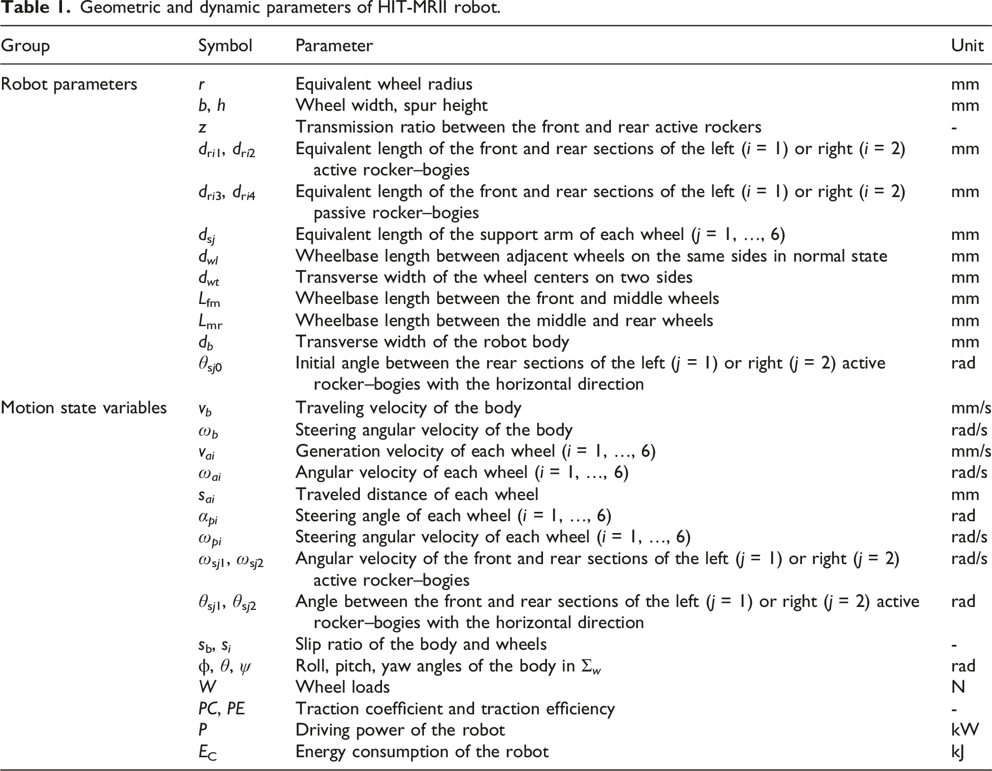
Geometric and dynamic parameters of HIT-MRII robot.

Group	Symbol	Parameter	Unit
Robot parameters	r	Equivalent wheel radius	mm
	b, h	Wheel width, spur height	mm
	z	Transmission ratio between the front and rear active rockers	-
	d_ri1, d_ri2	Equivalent length of the front and rear sections of the left (i = 1) or right (i = 2) active rocker–bogies	mm
	d_ri3, d_ri4	Equivalent length of the front and rear sections of the left (i = 1) or right (i = 2) passive rocker–bogies	mm
	d _sj	Equivalent length of the support arm of each wheel (j = 1, …, 6)	mm
	d _wl	Wheelbase length between adjacent wheels on the same sides in normal state	mm
	d _wt	Transverse width of the wheel centers on two sides	mm
	L _fm	Wheelbase length between the front and middle wheels	mm
	L _mr	Wheelbase length between the middle and rear wheels	mm
	d _b	Transverse width of the robot body	mm
	θ _sj0	Initial angle between the rear sections of the left (j = 1) or right (j = 2) active rocker–bogies with the horizontal direction	rad
Motion state variables	v _b	Traveling velocity of the body	mm/s
	ω _b	Steering angular velocity of the body	rad/s
	v _ai	Generation velocity of each wheel (i = 1, …, 6)	mm/s
	ω _ai	Angular velocity of each wheel (i = 1, …, 6)	rad/s
	s _ai	Traveled distance of each wheel	mm
	α _pi	Steering angle of each wheel (i = 1, …, 6)	rad
	ω _pi	Steering angular velocity of each wheel (i = 1, …, 6)	rad/s
	ω_sj1, ω_sj2	Angular velocity of the front and rear sections of the left (j = 1) or right (j = 2) active rocker–bogies	rad/s
	θ_sj1, θ_sj2	Angle between the front and rear sections of the left (j = 1) or right (j = 2) active rocker–bogies with the horizontal direction	rad
	s_b, s_i	Slip ratio of the body and wheels	-
	ϕ, θ, ψ	Roll, pitch, yaw angles of the body in Σ_w	rad
	W	Wheel loads	N
	PC, PE	Traction coefficient and traction efficiency	-
	P	Driving power of the robot	kW
	E _C	Energy consumption of the robot	kJ

2.1. Robot description

The SRWMR-APAS, named HIT-MRII robot, is equipped with six wheels and features two active single-input-multi-output (SIMO) joints—angle-adjusting mechanisms with actuators, as shown in Figure 2. In addition, it includes one passive SIMO joint without an actuator, resulting in a total of three SIMO joints with only two actuators. The passive SIMO joint functions as a differential mechanism connecting the left and right output shafts to the robot body, with its input considered zero. This differential mechanism ensures that the two output shafts rotate in opposite directions. Angle-adjusting mechanisms are employed to connect the output shafts with the front and rear segments of the rockers, maintaining the rotation angle at a certain proportion.

Figure 2.

Mechanical structure of the HIT-MRII robot (Qi et al., 2025a). Number 1 indicates the robot body; 2 indicates the front and back end of the actively articulated suspension rockers; 3 indicates the hinge point between the active rocker and the robot body; 4 indicates the front and back end of passively articulated suspension bogies; 5 indicates the clutch equipped at the joint point between the active and passive suspensions; 6 indicates wheel steering joint; 7 indicates wheel support arm; 8 indicates wheel driving joints; 9 indicates offset wheel; 10 indicates obstacle avoidance camera; 11 indicates navigation camera and mast; 12 indicates front-short-sighted radar; 13 indicates long-sighted navigation radar.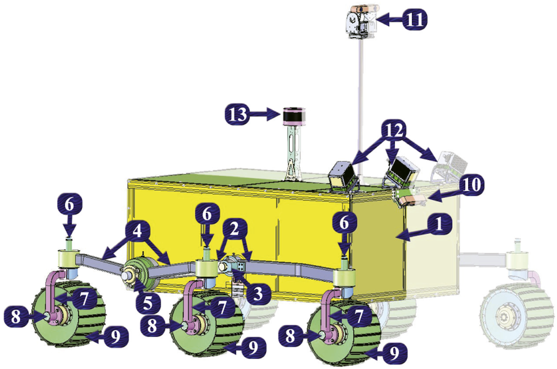

According to the number of robot joints, the top and lateral views of eight defined coordinate systems are depicted in Figures 3(b) and (c): world (Σ_w), body (Σ_b), central differential (Σ_d), active suspension hinged (Σ_s), passive suspension hinged (Σ_o), pillar (Σ_p), axis (Σ_a), and contact point (Σ_c). Furthermore, Σ_c plays a crucial role in responding to the contact state of the body posture and terrain undulation, which results from significant variations in the motion postures of the wheels on rough terrains.

Figure 3.

Attitudes and coordinate systems of the robot. *The coordinate systems related to the front wheels are Σ_w, Σ_b, Σ_d, Σ_s, Σ_p, Σ_a, and Σ_c; and the Σ_w, Σ_b, Σ_d, Σ_s, Σ_o, Σ_p, Σ_a, and Σ_c are related to the middle and rear wheels.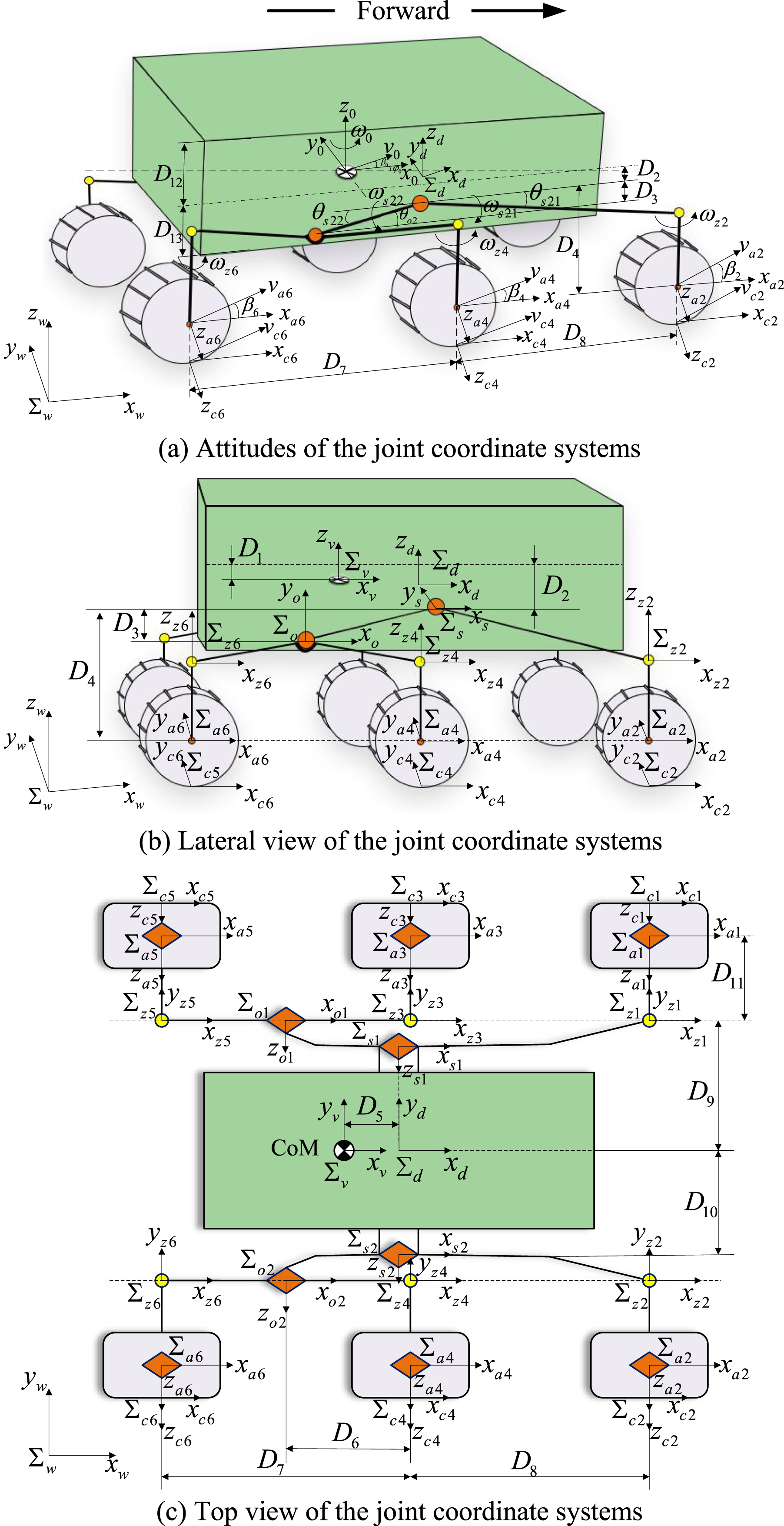

Given the hinged relation between each linkage of the robot, as shown in Figure 3(a), Σ_b can be moved slightly relative to Σ_d by the movement of other coordinate systems, and its origin presents the CoM position of the robot. In addition, the motion constraints below are defined, in the next two sections, to limit the movement to a small range. Consequently, this movement is not taken into account in the velocity mapping. The remaining joints exclusively possess rotational motion. Specifically, 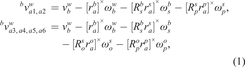$v_{d}^{b} = v_{s}^{d} = v_{p}^{s} = v_{a}^{p} = ω_{a}^{p} = 0$ and $v_{d}^{b} = v_{s}^{d} = v_{o}^{s} = v_{p}^{o} = v_{a}^{p} = ω_{a}^{p} = 0$ . The velocities of the front offset wheel center and those of the middle and rear offset wheel centers relative to Σ_w in Σ_b are derived by

\begin{aligned} {}^{b}v_{a 1, a 2}^{w} & = v_{b}^{w} - {[r_{a}^{b}]}^{\times} ω_{b}^{w} - {[R_{s}^{b} r_{a}^{s}]}^{\times} ω_{s}^{b} - {[R_{p}^{s} r_{a}^{p}]}^{\times} ω_{p}^{s}, \\ {}^{b}v_{a 3, a 4, a 5, a 6}^{w} & = v_{b}^{w} - {[r_{a}^{b}]}^{\times} ω_{b}^{w} - {[R_{s}^{b} r_{a}^{s}]}^{\times} ω_{s}^{b} \\ - {[R_{o}^{s} r_{a}^{o}]}^{\times} ω_{o}^{s} - {[R_{p}^{o} r_{a}^{p}]}^{\times} ω_{p}^{o}, \end{aligned}

(1)

where

r_{a}^{b}

r_{a}^{s}

r_{a}^{p}

, and

r_{a}^{o}

are the position vectors of coordinate system Σ_a relative to Σ_b, Σ_s, Σ_p, and Σ_o, respectively.

R_{s}^{b}

R_{p}^{s}

R_{o}^{s}

, and

R_{p}^{o}

represent the rotation transform matrices from Σ_s to Σ_b, from Σ_p to Σ_s, from Σ_o to Σ_s, and from Σ_p to Σ_o, respectively.

The hinge-point rotation angle of the active suspension in Σ_s is defined as γ, and that of the passive suspension in Σ_o is denoted as ζ. The rotation angles of the wheel support arm in Σ_p and the wheel center in Σ_a are defined as μ and ɛ, respectively; then, the velocities of the contact points of the front offset wheels and those of the middle and rear offset wheels relative to Σ_w in Σ_b are derived by equation (1) as follows: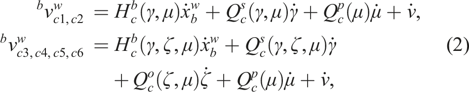

\begin{aligned} {}^{b}v_{c 1, c 2}^{w} & = H_{c}^{b} (γ, μ) {\dot{x}}_{b}^{w} + Q_{c}^{s} (γ, μ) \dot{γ} + Q_{c}^{p} (μ) \dot{μ} + \dot{ν}, \\ {}^{b}v_{c 3, c 4, c 5, c 6}^{w} & = H_{c}^{b} (γ, ζ, μ) {\dot{x}}_{b}^{w} + Q_{c}^{s} (γ, ζ, μ) \dot{γ} \\ + Q_{c}^{o} (ζ, μ) \dot{ζ} + Q_{c}^{p} (μ) \dot{μ} + \dot{ν}, \end{aligned}

(2)

where

{\dot{x}}_{b}^{w} = {[\begin{matrix} {(v_{b}^{w})}^{T} & {(ω_{b}^{w})}^{T} \end{matrix}]}^{T}

contains the linear velocity and angular velocity of the robot;

H_{c}^{b} = [I | - {[r_{a}^{b}]}^{\times}]

is the transformation matrix from the body velocity

{\dot{x}}_{b}

to the wheel–terrain contact point velocities;

Q_{c}^{s} (γ, μ) = - {[R_{s}^{b} r_{a}^{s}]}^{\times}

and

Q_{c}^{p} (μ) = - {[R_{p}^{s} r_{a}^{p}]}^{\times}

are the transformation matrices of front offset wheels from angular velocities

\dot{γ}

and

\dot{μ}

to the contact point velocities in Σ_b; while

Q_{c}^{s} (γ, ζ, μ) = - {[R_{s}^{b} r_{a}^{s}]}^{\times}

Q_{c}^{o} (ζ, μ) = - {[R_{o}^{s} r_{a}^{o}]}^{\times}

, and

Q_{c}^{p} (μ) = - {[R_{p}^{o} r_{a}^{p}]}^{\times}

are the corresponding transformation matrices of middle and rear offset wheels from angular velocities

\dot{γ}

\dot{ζ}

, and

\dot{μ}

to the contact point velocities in Σ_b;

\dot{γ} = ω_{s}^{b}

and

\dot{ζ} = ω_{o}^{s}

are the angular velocities of the actively and passively articulated suspension hinge-joint point, respectively;

\dot{μ} = ω_{p}^{s}

(

\dot{μ} = ω_{p}^{o}

) is the wheel support-arm hinge-joint angular velocity of the front (middle and rear) wheels; and

\dot{ν} = v_{c}^{a}

is the velocity of the contact point relative to the wheel center.

2.2. Differential steering model taking into account the variable wheelbase length

Utilizing the instantaneous center (IC) method, a 3D kinematic model of differential steering was developed to achieve the motion with variable instantaneous steering radii of the wheels while the robot is in motion, resulting from adjusting the angle of the active rocker–bogies and the corresponding wheelbase length. Consequently, the locations of the IC, whether on or off the longitudinal central axis of the body, are shown in Figures 4(a) and (b), respectively.

Figure 4.

IC axial models of differential steering.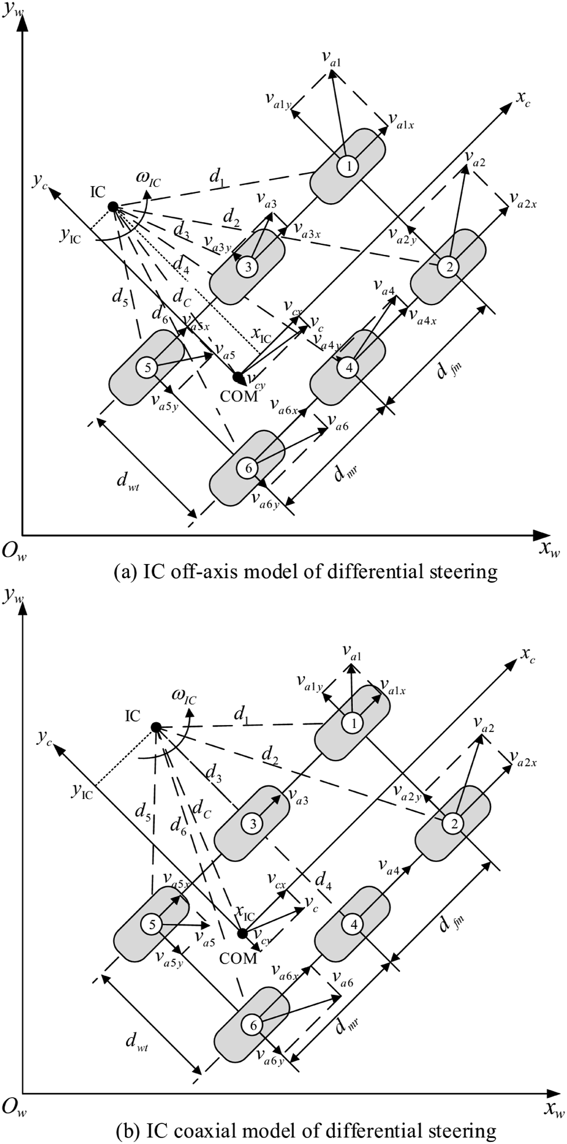

Assuming a symmetric distribution of mass on the left and right sides of the robot body, the CoM is initially located on the central axis of these sides. Let L_ox denote the offset between the robot body’s CoM and its centroid in the front-rear direction. In the initial state, the wheelbase length between the front and middle wheels equals that of the middle and rear wheels. The IC is positioned on the extended line of the central axis, with coordinates $(L_{o x}, \frac{v_{R}^{2} - v_{L}^{2}}{2 ω_{b}^{2} d_{w t}})$ with v_L and v_R denoting the linear velocities of the wheels on the left and right sides, as shown in Figure 4(a). When both suspensions move synchronously, the IC is positioned at the midpoint of the wheelbase length between the front and rear wheels. Consequently, the coordinates of the IC in Σ_b are $(L_{o x} - \frac{L_{wb i}}{2}, \frac{v_{R}^{2} - v_{L}^{2}}{2 ω_{b}^{2} d_{w t}})$ , where i = 1, 2, and L_wbi is the variation in the front-middle wheelbase lengths.

The following regular part of the derivation of the differential velocity model is shown in Appendix A. Furthermore, when the equivalent radii of the wheels are equal, that is, r_i = r, i = 1, 2, …, 6, we have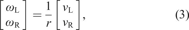

[\begin{matrix} ω_{L} \\ ω_{R} \end{matrix}] = \frac{1}{r} [\begin{matrix} v_{L} \\ v_{R} \end{matrix}],

(3)

where ω_L and ω_R are the angular velocities of the wheels on the left and right sides of the body, respectively.

Taking into account the defined motion constraints between the multi-joints in the robot (equations (19) and (20)), the linear and angular velocities of the body mapped from the angular velocities of the wheels and active rocker–bogies are given, as follows: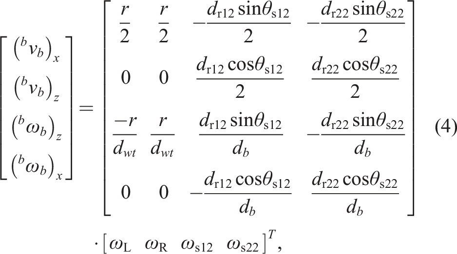

\begin{aligned} [\begin{matrix} {({}^{b}v_{b})}_{x} \\ {({}^{b}v_{b})}_{z} \\ {({}^{b}ω_{b})}_{z} \\ {({}^{b}ω_{b})}_{x} \end{matrix}] & = [\begin{matrix} \frac{r}{2} & \frac{r}{2} & - \frac{d_{r 12} \sin θ_{s 12}}{2} & - \frac{d_{r 22} \sin θ_{s 22}}{2} \\ 0 & 0 & \frac{d_{r 12} \cos θ_{s 12}}{2} & \frac{d_{r 22} \cos θ_{s 22}}{2} \\ \frac{- r}{d_{w t}} & \frac{r}{d_{w t}} & \frac{d_{r 12} \sin θ_{s 12}}{d_{b}} & - \frac{d_{r 22} \sin θ_{s 22}}{d_{b}} \\ 0 & 0 & - \frac{d_{r 12} \cos θ_{s 12}}{d_{b}} & \frac{d_{r 22} \cos θ_{s 22}}{d_{b}} \end{matrix}] \\ \cdot {[\begin{matrix} ω_{L} & ω_{R} & ω_{s 12} & ω_{s 22} \end{matrix}]}^{T}, \end{aligned}

(4)

where

{({}^{b}v_{b})}_{x}

{({}^{b}v_{b})}_{z}

{({}^{b}ω_{b})}_{z}

, and

{({}^{b}ω_{b})}_{x}

denote the forward, vertical, steering angular, and lateral angular velocities of the robot in body coordinate system Σ_b, respectively; ω_s12 and ω_s22 represent the angular velocities of the rear active rockers on the left and right sides of the body; θ_s12 and θ_s22 are the angles between the left and right rear active rockers and the horizontal direction; d_r12 and d_r22 represent the lengths of the left and right rear active rockers.

The coordinate transformation that converts the velocity coordinates from Σ_b to Σ_w is given by equation (5),

[\begin{matrix} {({}^{w}v_{b})}_{x} \\ {({}^{w}v_{b})}_{y} \\ {({}^{w}v_{b})}_{z} \end{matrix}] = [\begin{matrix} \cos ψ \cos θ & \cos ψ \sin θ \sin ϕ - \sin ψ \cos ϕ & \cos ψ \sin θ \cos ϕ + \sin ψ \sin ϕ \\ \sin ψ \cos θ & \sin ψ \sin θ \sin ϕ + \cos ψ \cos ϕ & \sin ψ \sin θ \cos ϕ - \cos ψ \sin ϕ \\ - \sin θ & \cos θ \sin ϕ & \cos θ \cos ϕ \end{matrix}] [\begin{matrix} {({}^{b}v_{b})}_{x} \\ {({}^{b}v_{b})}_{y} \\ {({}^{b}v_{b})}_{z} \end{matrix}] .

(5)

where ${({}^{w}v_{b})}_{x}$ , ${({}^{w}v_{b})}_{y}$ , and ${({}^{w}v_{b})}_{z}$ represent the x-, y-, and z-components of the linear velocity of the robot CoM in Σ_w. Then, the coordinate transformation that converts angular velocity coordinates in Σ_b to derivatives of the Euler angles of the robot body in Σ_w is given, as follows:

[\begin{matrix} \dot{ϕ} \\ \dot{θ} \\ \dot{ψ} \end{matrix}] = [\begin{matrix} 1 & \sin ϕ \tan θ & \cos ϕ \tan θ \\ 0 & \cos ϕ & - \sin ϕ \\ 0 & \sin ϕ / \cos θ & \cos ϕ / \cos θ \end{matrix}] [\begin{matrix} {({}^{b}ω_{b})}_{x} \\ {({}^{b}ω_{b})}_{y} \\ {({}^{b}ω_{b})}_{z} \end{matrix}],

(6)

where ϕ, θ, and ψ are the roll, pitch, and yaw angles of the robot body in Σ_w.

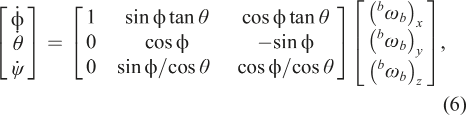
The forward 3D kinematic model in Σ_w is described as follows: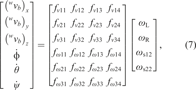

[\begin{matrix} {({}^{w}v_{b})}_{x} \\ {({}^{w}v_{b})}_{y} \\ {({}^{w}v_{b})}_{z} \\ \dot{ϕ} \\ \dot{θ} \\ \dot{ψ} \end{matrix}] = [\begin{matrix} f_{v11} & f_{v12} & f_{v13} & f_{v14} \\ f_{v21} & f_{v22} & f_{v23} & f_{v24} \\ f_{v31} & f_{v32} & f_{v33} & f_{v34} \\ f_{ω 11} & f_{ω 12} & f_{ω 13} & f_{ω 14} \\ f_{ω 21} & f_{ω 22} & f_{ω 23} & f_{ω 24} \\ f_{ω 31} & f_{ω 32} & f_{ω 33} & f_{ω 34} \end{matrix}] [\begin{matrix} ω_{L} \\ ω_{R} \\ ω_{s 12} \\ ω_{s 22} \end{matrix}],

(7)

where the matrix parameters are provided in Appendix B.

In addition, the relation between the height of the lifted wheels off the ground and the rotation angle of the active rocker–bogies are given as follows:

(1) The height h_fw in the case of the front-wheel lifting can be calculated as follows:

\begin{aligned} h_{fw} & = \sqrt{d_{r i 1}^{2} + d_{s j}^{2}} [\sin (α_{sf} + z ω_{s i 2} t - z θ_{s i 0}) \\ - \sin (α_{sf} - ω_{s i 2} t + θ_{s i 0})], \end{aligned}

(8)

where t denotes the operation duration; h_fw denotes the height of the front wheel off the ground; d_ri1 is the length of the front section of the active rocker with i = 1, 2 indicating the left- and right-side of the robot body; d_sj is the length of the support arms connecting with the front wheels with j = 1, 2 represents the left- and right-side; θ_si0 is the initial angle between the rear sections of the left (i = 1) or right (i = 2) active rocker–bogies with the horizontal direction; α_sf is the angle between the front section of the active rocker and the line connecting the front wheel and the hinge point between the active rocker and the robot body, which is calculated by

α_{sf} = \tan^{- 1} \frac{d_{s j}}{d_{r i 1}} .

(2) The height h_mw in the case of the middle-wheel lifting can be calculated as follows:

\begin{aligned} h_{mw} & = d_{om} \cos β_{mw} [\sin (α_{om} - θ_{s i 0} + ω_{s i 2} t) \\ - \sin (α_{om} - θ_{s i 0} - ω_{s i 2} t)], \\ d_{om} & = \sqrt{d_{r i 3}^{2} + d_{s j}^{2} - 2 d_{r i 3} d_{s j} \sin θ_{s i 0}}, \end{aligned}

(9)

where h_mw denotes the height of the middle wheel off the ground; d_ri3 is the length of the front section of the passive bogie with i = 1, 2 indicating the left- and right-side of the robot body; d_sj is the length of the support arms connecting with the middle wheels with j = 3, 4 represents the left- and right-side; d_om represents the length of the line connecting the middle wheel and the hinge of the actively and passively articulated suspensions, and α_om is the angle between this line and the front section of the passive bogie, which is calculated as follows:

α_{om} = \tan^{- 1} \frac{d_{s j} - d_{r i 3} \sin θ_{s i 0}}{d_{r i 3} \cos θ_{s i 0}} + θ_{s i 0},

and β_mw is the change in the pitch angle of the robot resulting from the lifting motion of the middle wheel, which can be estimated by the following equation:

\begin{aligned} β_{mw} = \\ \tan^{- 1} \frac{d_{om} [\sin (α_{om} + ω_{s i 2} t) - \sin α_{om}]}{L_{fm} + L_{mr} - L_{wb i} - d_{om} [\cos α_{om} - \cos (α_{om} + ω_{s i 2} t)]}, \end{aligned}

where L_wbi represents the variation in the wheelbase length between the right front and middle wheels with i = 1, 2 indicating the left- and right-side.

(3) The height h_rw in the case of the rear-wheel lifting can be calculated as follows:

\begin{aligned} h_{rw} & = d_{or} \cos β_{rw} [\sin (α_{or} - θ_{s i 0} + ω_{s i 2} t) \\ - \sin (α_{or} - θ_{s i 0} - ω_{s i 2} t)], \\ d_{or} & = \sqrt{d_{r i 4}^{2} + d_{s j}^{2} - 2 d_{r i 4} d_{s j} \sin θ_{s i 0}}, \end{aligned}

(10)

where h_rw denotes the height of the rear wheel off the ground; d_ri4 is the length of the rear section of the passive bogie with i = 1, 2 indicating the left- and right-side of the robot body; d_sj is the length of the support arms connecting with the rear wheels with j = 5, 6 represents the left- and right-side; d_or represents the length of the line connecting the rear wheel and the hinge of the actively and passively articulated suspensions, and α_or is the angle between this line and the rear section of the passive bogie, which is calculated as follows:

α_{or} = \tan^{- 1} \frac{d_{s j} - d_{r i 4} \sin θ_{s i 0}}{d_{r i 4} \cos θ_{s i 0}} + θ_{s i 0},

and β_rw is the change in the pitch angle of the robot resulting from the lifting motion of the rear wheel, which can be estimated by the following equation:

β_{rw} = \tan^{- 1} \frac{d_{or} [\sin (α_{or} + ω_{s i 2} t) - \sin α_{or}]}{L_{fm} + d_{or} [\cos α_{or} - \cos (α_{or} + ω_{s i 2} t)]} .

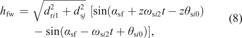
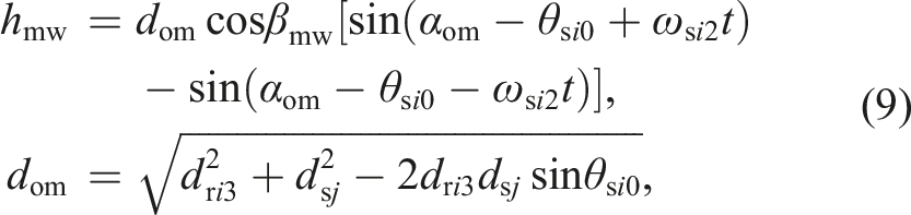
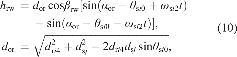
The desired lifting height can be calculated from equations (8)–(10), and the corresponding wheel motion is then generated using the established kinematic model in equation (7).

3. Constraints for joint coordination in multimode motion

The achievable morphologies of HIT-MRII robot are categorized by its active and passive suspension articulations, and the proposed optimization generates feasible commands to realize them across motion modes. Motion constraints are imposed to coordinate coupled joints, and to maintain safe geometric/contact conditions during mode execution and action transitions.

The multimode can be divided into two categories: wheel motion, and wheel-suspension hybrid control. In consequence, six typical motion modes of the SRWMR-APAS are defined as Wheel Rolling Mode (WRM), Wheel Crabbing Mode (WCM), Robot Chassis Lifting Mode (RCLM), Robot Creeping Mode (RCM), Single Wheel Lifting Mode (SWLM), and Double Wheel Lifting Mode (DWLM). Their control processes and objectives are summarized in Table 2. Moreover, in the specialized motion design of these modes, the RCM is characterized by the continuous cycle in the RCLM, while they have different rotation directions of wheels. Both the SWLM and DWLM share the same control sequence, while they differ in the number of driving motors. Consequently, the WCM, RCLM, RCM, and DWLM as representatives are shown in Figure 5.

Table 2.

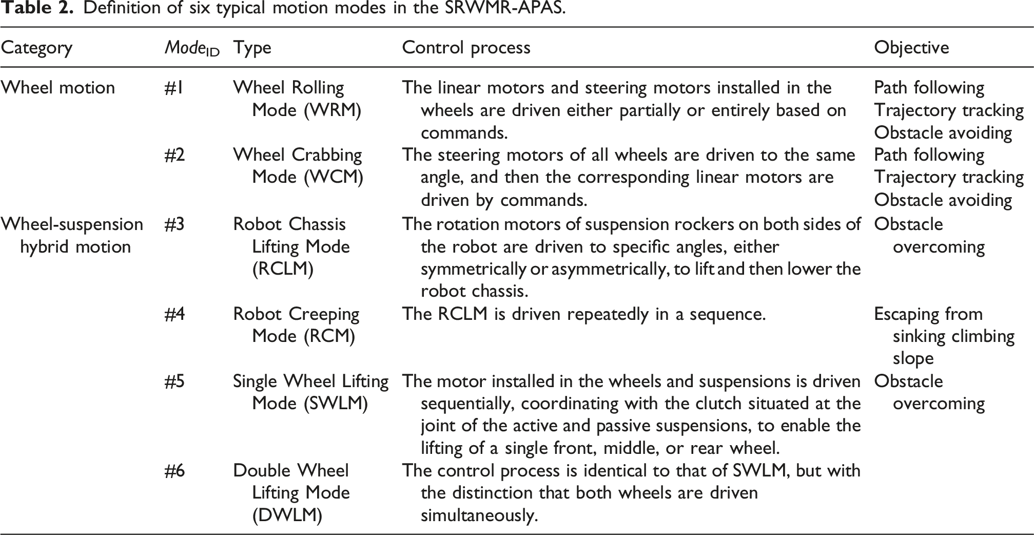
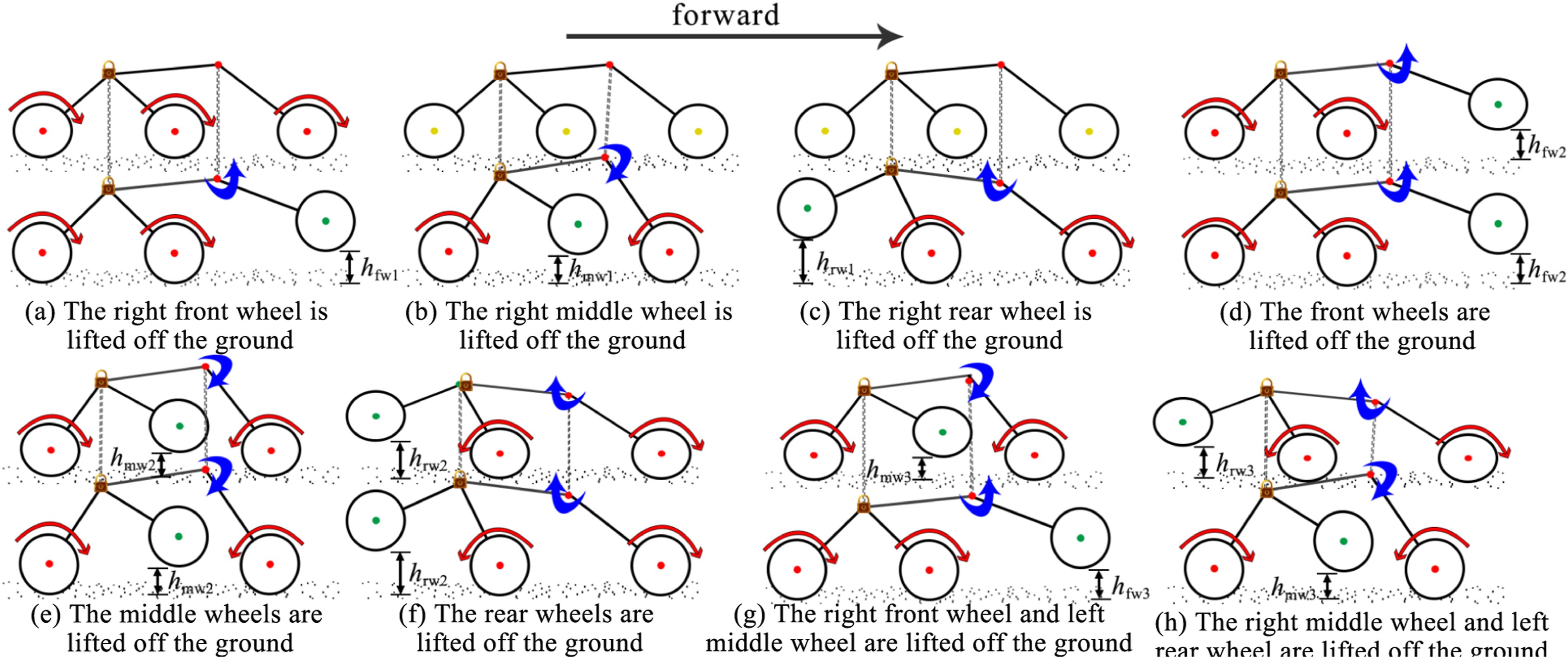
Definition of six typical motion modes in the SRWMR-APAS.

Category	Mode _ID	Type	Control process	Objective
Wheel motion	#1	Wheel Rolling Mode (WRM)	The linear motors and steering motors installed in the wheels are driven either partially or entirely based on commands.	Path following
				Trajectory tracking
				Obstacle avoiding
	#2	Wheel Crabbing Mode (WCM)	The steering motors of all wheels are driven to the same angle, and then the corresponding linear motors are driven by commands.	Path following
				Trajectory tracking
				Obstacle avoiding
Wheel-suspension hybrid motion	#3	Robot Chassis Lifting Mode (RCLM)	The rotation motors of suspension rockers on both sides of the robot are driven to specific angles, either symmetrically or asymmetrically, to lift and then lower the robot chassis.	Obstacle overcoming
	#4	Robot Creeping Mode (RCM)	The RCLM is driven repeatedly in a sequence.	Escaping from sinking climbing slope
	#5	Single Wheel Lifting Mode (SWLM)	The motor installed in the wheels and suspensions is driven sequentially, coordinating with the clutch situated at the joint of the active and passive suspensions, to enable the lifting of a single front, middle, or rear wheel.	Obstacle overcoming
	#6	Double Wheel Lifting Mode (DWLM)	The control process is identical to that of SWLM, but with the distinction that both wheels are driven simultaneously.	Obstacle overcoming

Figure 5.

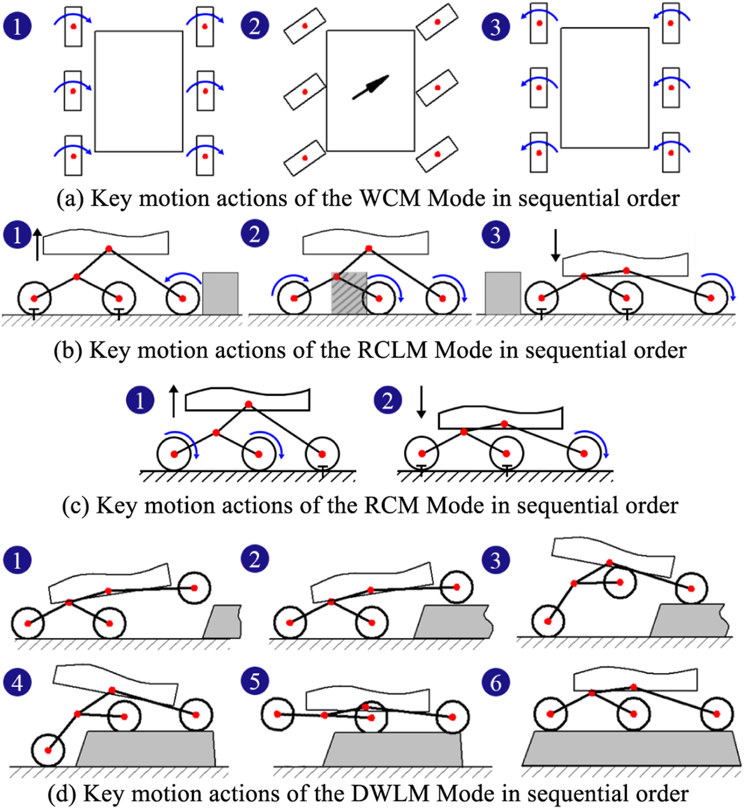
Illustrations of control processes in Wheel Crabbing Mode (WCM), Robot Chassis Lifting Mode (RCLM), Robot Creeping Mode (RCM), and Double Wheel Lifting Mode (DWLM). For the mutual inclusion relation between the modes, WRM is utilized as the action ② of WCM and RCLM; the actions ① and ③ of RCLM are utilized as the actions ① and ② of RCM; WRM is utilized as the actions ②, ④, and ⑥ of DWLM and SWLM; The lifting actions are utilized as actions ①, ③, and ⑤ of DWLM and SWLM.

3.1. Anti body-posture instability constraints in wheel lifting scenarios

In the multimode motion of the SRWMR-APAS, the lifting of a wheel from the ground is conventionally executed by the active suspension system, leading to the achievement of specialized functionalities, such as obstacle avoidance. In addition, to effectively adapt to varying terrain undulations, the lifting can be changed by passive suspension mechanisms. As shown in equation (2), the specific combinations of wheel numbers and positions are presented within the kinematic model.

To ensure motion stability in the cases of lifting wheels, the first Motion Constraint #1 is defined for the wheels in the HIT-MRII robot, including three rules: (1) no more than two wheels can be lifted at once; (2) front and rear wheels cannot be lifted simultaneously; (3) only one wheel can be lifted on each side of the body. Accordingly, wheel-lifting cases are categorized into three distinct groups for HIT-MRII robot in the modeling: the lifting of a single wheel, denoted as c₁, c₂, c₃, c₄, c₅, or c₆ from the ground; the lifting of two symmetric wheels, denoted as c₁c₂, c₃c₄, or c₅c₆ from the ground; and the lifting of two asymmetric wheels, denoted as c₁c₄, c₂c₃, c₃c₆, or c₄c₅ from the ground. Moreover, a reconstruction of the kinematic model becomes necessary in cases of wheel-lifting motions.

According to the mechanical characteristics of the HIT-MRII, the wheels are lifted by controlling the active suspension motion and the connection of the clutch positioned at the hinge of the actively and passively articulated suspensions. In the cases of lifting wheels, when the robot body’s CoM is positioned in the front or rear of the body box, the rear or front wheels can be lifted, respectively. In addition, the CoM does not affect the lifting of the middle wheel. Furthermore, when a single wheel is lifted, the posture of the active suspension on both sides of the robot is no longer symmetrical, resulting in the CoM shifting to the side of the unlifted wheel; when two symmetrical wheels are lifted, the six-wheeled motion model can be simplified to the four-wheeled model; in addition, symmetric and asymmetric postures of both sides of the robot are possible when two asymmetric wheels are lifted.

Remark 1

When a wheel is lifted just off the ground surface, resulting in zero contact force but minimal position change, parts of the wheels are caused to sink deeper into loose soil due to the asymmetric wheel distribution and load redistribution. The body box is caused to tilt. The initial movement of the CoM position is induced by the tilting motion of the body. As the lifting height increases, the CoM position is further changed by the wheel-suspension motion.

In cases where wheel i is lifted, the motion efficiency of the corresponding Σc_i within the general kinematic model, as described in equation (2), is decreased due to ineffective driving. Consequently, based on the defined Motion Constraint #1, the three wheel-lifting patterns of HIT-MRII are shown in Figure 6, and analyzed as follows:

(1) A single front, middle, or rear wheel is lifted, as shown in Figures 6(a)−(c), respectively. The changed parameters of the kinematics are the number of wheels n, the angle between the front and rear ends of the active rocker–bogies γ, and the angle between the rear section of the active rocker–bogies and the auxiliary rocker–bogies ζ. For example, in the case where the right front wheel is lifted, ${}^{b}v_{c 2}^{w} = 0$ , and the velocities of the contact points of the remaining offset wheels are calculated by equation (2);

(2) Both front, middle, or rear symmetric wheels are lifted, as shown in Figures 6(d) −(f), respectively. In the case where both middle wheels are lifted, ${}^{b}v_{c 3}^{w} = {}^{b}v_{c 4}^{w} = 0$ , and the velocities of the contact points of the remaining offset wheels are calculated by equation (2);

(3) Two asymmetric front, middle, or rear wheels are lifted, as shown in Figures 6(g) and (h). In the case where the left middle and right front wheels are lifted, ${}^{b}v_{c 2}^{w} = {}^{b}v_{c 3}^{w} = 0$ , and the velocities of the contact points of the remaining offset wheels are calculated by equation (2).

Figure 6.

Partial wheel is lifted off the ground. In the subfigures, the enable state, disable state, and still state are indicated by the red, green, and yellow dots, respectively. In addition, the blue arrow denotes the direction of suspension movement. The lifted height is represented by h.

3.2. Anti-slippage constraints for the jointed wheels during active suspension-rocker movement

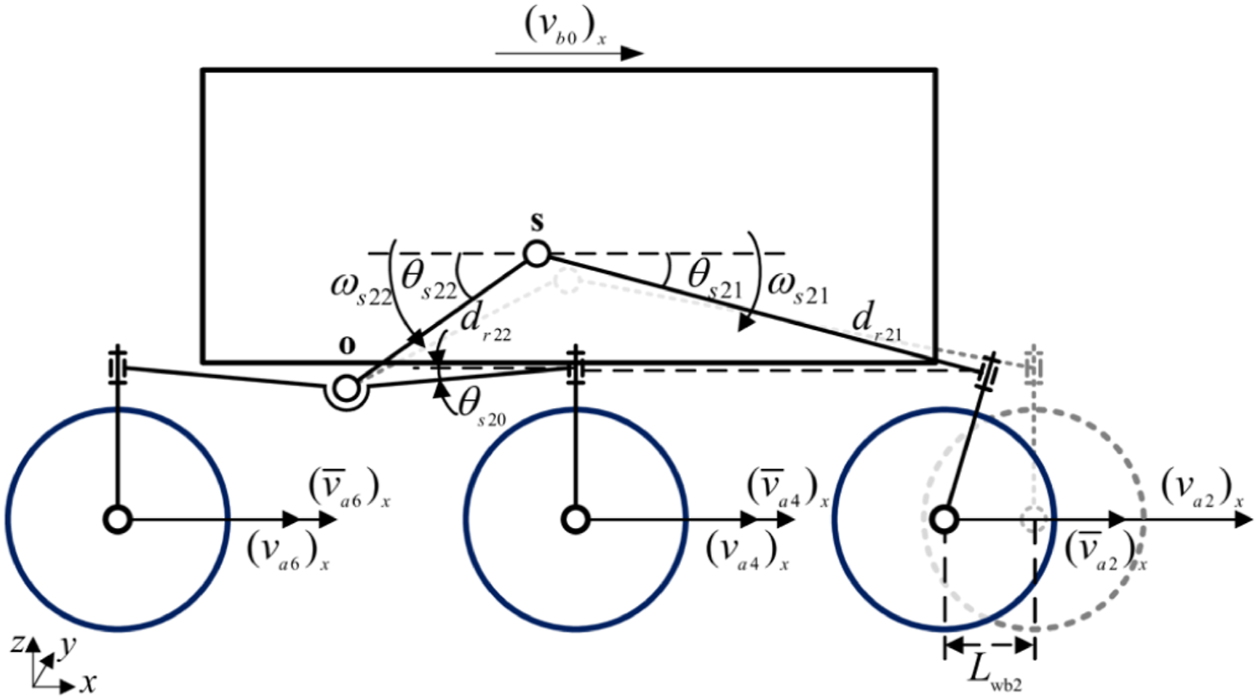
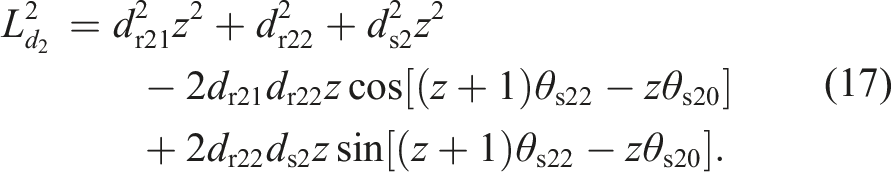
The dangerous situations of severe wheel slippage and the robot rollover are more likely caused by the lack of coordination in velocities between the wheels and suspension rocker–bogies. For the suspension systems, the nominal state is defined as the condition in which the front section of the active suspension’s rocker is aligned parallel to the horizontal line, while the rear half of the rocker is coplanar with the front half of the passive suspension. In this state, the angle formed between the initial direction of the rear section of the active rocker on the right (left) side and the horizontal direction is represented by θ_s20 (θ_s10). Consequently, the angle variation of the rear section of the active suspension rocker is described as θ_s22 (θ_s12) − θ_s20 (θ_s10), as illustrated in Figure 7. Moreover, the transmission relation of the angular velocity between the front and rear sections of the active rockers is defined as follows:

ω_{s 21} = z ω_{s 22},

(11)

where z is the transmission ratio between the front and rear sections of the active rockers.

Figure 7.

Wheelbase-length variation induced by the front half of the active rocker.

In addition, angles of the front and rear sections of the active suspension rockers satisfy the following relation:

θ_{s 21} = z (θ_{s 22} - θ_{s 20}) .

(12)

The changed wheelbase length between the front and middle wheels by the right suspension motion is shown in Figure 7.

Then, the following geometric relation of the suspension can be derived as follows: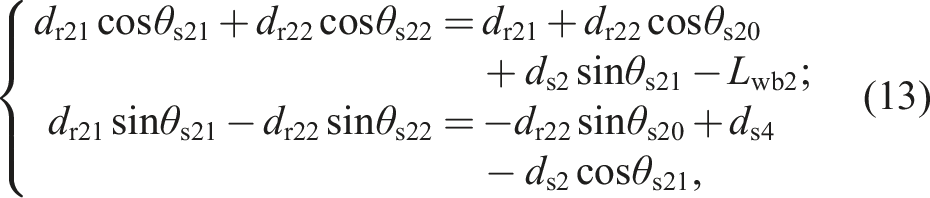

\{\begin{aligned} d_{r 21} \cos θ_{s 21} + d_{r 22} \cos θ_{s 22} & = d_{r 21} + d_{r 22} \cos θ_{s 20} \\ + d_{s 2} \sin θ_{s 21} - L_{wb 2}; \\ d_{r 21} \sin θ_{s 21} - d_{r 22} \sin θ_{s 22} & = - d_{r 22} \sin θ_{s 20} + d_{s 4} \\ - d_{s 2} \cos θ_{s 21}, \end{aligned}

(13)

where L_wb2 is the variation in the wheelbase length between the right front and middle wheels; d_s2 and d_s4 are the lengths of support arms of the right front and middle wheels, and by structural design, d_s2 = d_s4.

The derivative of equation (13) with respect to t is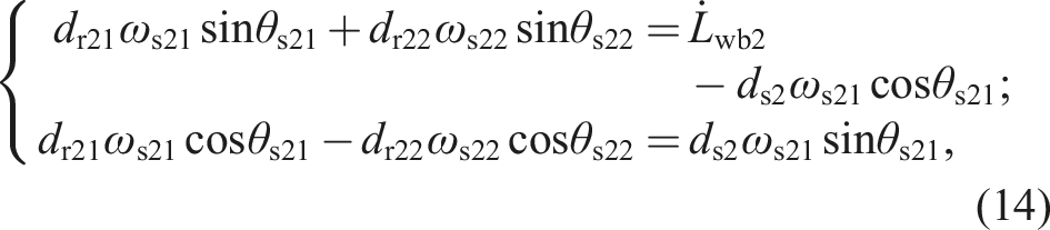

\{\begin{aligned} d_{r 21} ω_{s 21} \sin θ_{s 21} + d_{r 22} ω_{s 22} \sin θ_{s 22} & = {\dot{L}}_{wb 2} \\ - d_{s 2} ω_{s 21} \cos θ_{s 21}; \\ d_{r 21} ω_{s 21} \cos θ_{s 21} - d_{r 22} ω_{s 22} \cos θ_{s 22} & = d_{s 2} ω_{s 21} \sin θ_{s 21}, \end{aligned}

(14)

where

{\dot{L}}_{wb 2} = {(v_{a 4})}_{x} - {(v_{a 2})}_{x}

, and

{\dot{L}}_{wb 2}

is the rate of change of the wheelbase length between the front and middle wheels caused by the different velocities of the right middle and front wheels.

To calculate the increment of linear velocity of the wheels generated by the motion of the active rocker–bogies in the forward direction, the squares of the two formulas in equation (14) are summed as follows: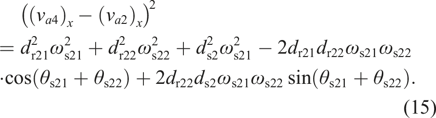

\begin{aligned} {({(v_{a 4})}_{x} - {(v_{a 2})}_{x})}^{2} \\ = d_{r 21}^{2} ω_{s 21}^{2} + d_{r 22}^{2} ω_{s 22}^{2} + d_{s 2}^{2} ω_{s 21}^{2} - 2 d_{r 21} d_{r 22} ω_{s 21} ω_{s 22} \\ \cdot \cos (θ_{s 21} + θ_{s 22}) + 2 d_{r 22} d_{s 2} ω_{s 21} ω_{s 22} \sin (θ_{s 21} + θ_{s 22}) . \end{aligned}

(15)

Equations (11) and (12) are substituted into equation (14) to eliminate θ_s21 and ω_s21, the conversion relation between the angular velocities of the active rocker–bogies and the velocity difference between the front and middle wheels is obtained as follows:

Δ {(v_{a R})}_{x} = L_{d_{2}} ∣ ω_{s 22} ∣,

(16)

where

Δ {(v_{a R})}_{x} = {(v_{a 4})}_{x} - {(v_{a 2})}_{x}

denotes the velocity difference between the right front and middle wheels, and

L_{d_{2}}

is solved by the following equation:

\begin{aligned} L_{d_{2}}^{2} & = d_{r 21}^{2} z^{2} + d_{r 22}^{2} + d_{s 2}^{2} z^{2} \\ - 2 d_{r 21} d_{r 22} z \cos [(z + 1) θ_{s 22} - z θ_{s 20}] \\ + 2 d_{r 22} d_{s 2} z \sin [(z + 1) θ_{s 22} - z θ_{s 20}] . \end{aligned}

(17)

To enhance the coordination of motion between wheels and active suspension rockers, the change in velocities of the jointed wheel relative to the active-rocker motion can be determined by Motion Constraint #2, as specified by equation (16). The definition and objective of all defined motion constraints are listed in Table 3.

Table 3.

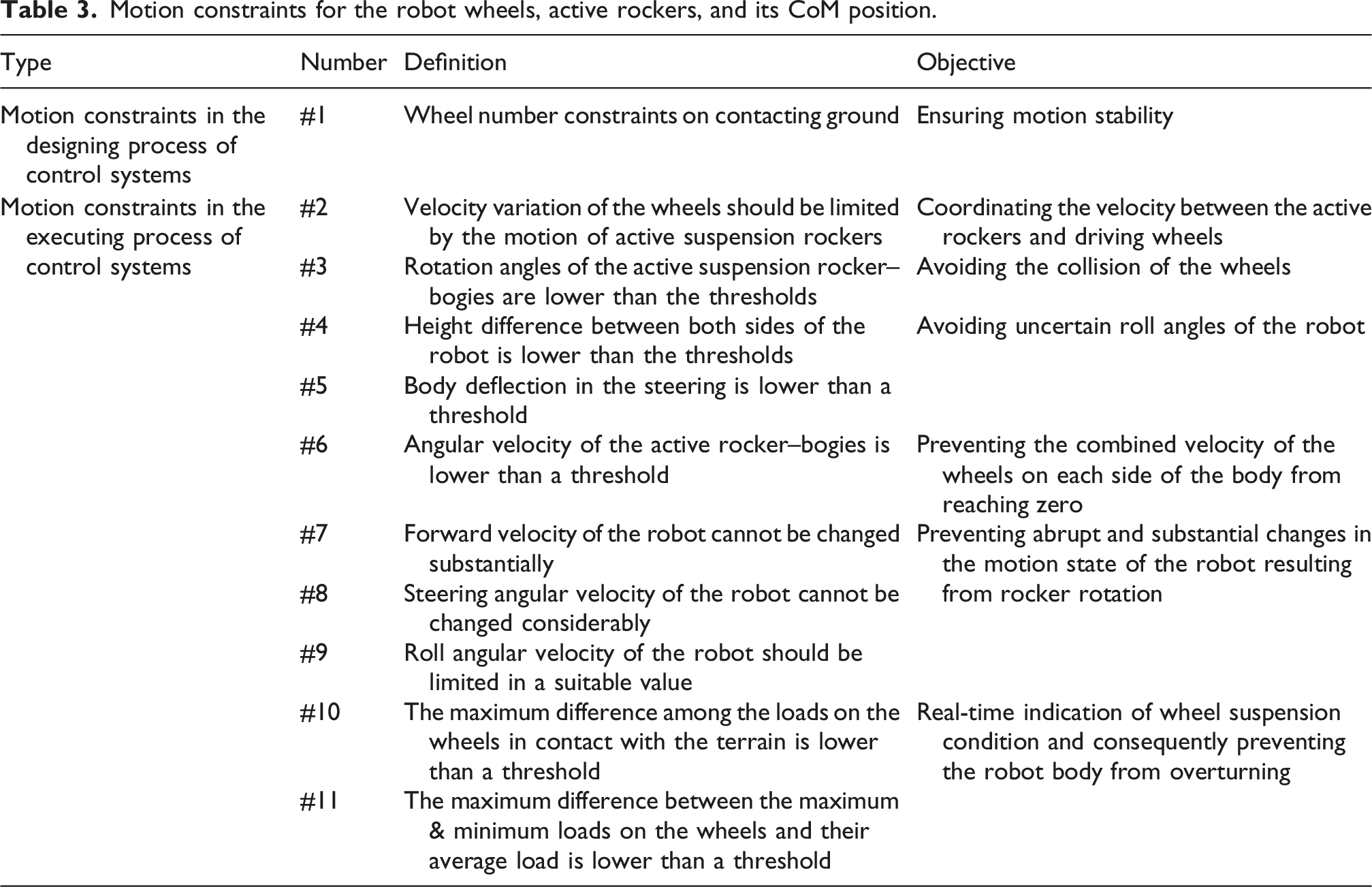
Motion constraints for the robot wheels, active rockers, and its CoM position.

Type	Number	Definition	Objective
Motion constraints in the designing process of control systems	#1	Wheel number constraints on contacting ground	Ensuring motion stability
Motion constraints in the executing process of control systems	#2	Velocity variation of the wheels should be limited by the motion of active suspension rockers	Coordinating the velocity between the active rockers and driving wheels
	#3	Rotation angles of the active suspension rocker–bogies are lower than the thresholds	Avoiding the collision of the wheels
	#4	Height difference between both sides of the robot is lower than the thresholds	Avoiding uncertain roll angles of the robot
	#5	Body deflection in the steering is lower than a threshold	Avoiding uncertain roll angles of the robot
	#6	Angular velocity of the active rocker–bogies is lower than a threshold	Preventing the combined velocity of the wheels on each side of the body from reaching zero
	#7	Forward velocity of the robot cannot be changed substantially	Preventing abrupt and substantial changes in the motion state of the robot resulting from rocker rotation
	#8	Steering angular velocity of the robot cannot be changed considerably
	#9	Roll angular velocity of the robot should be limited in a suitable value
	#10	The maximum difference among the loads on the wheels in contact with the terrain is lower than a threshold	Real-time indication of wheel suspension condition and consequently preventing the robot body from overturning
	#11	The maximum difference between the maximum & minimum loads on the wheels and their average load is lower than a threshold

4. Constraints for the moving range of the robot CoM in multimode motion

To ensure the robot’s posture stability during multimode motion, the corresponding motion constraints are defined to manage the moving range of the robot’s CoM by controlling the relative lifting distance of both sides of the body and their relative velocity, in this section.

The forward and upward increment velocities of the body CoM can be generated with the movements of suspension rocker–bogies. In the cases of asymmetrical movement in the suspensions on both sides of the robot, the body CoM can deviate from the transverse centerline, under an assumption of initially symmetric mass distribution. This deviation induces a lateral offset, resulting in decreased stability.

Moreover, in cases where a single middle or rear wheel is lifted, the articulated design of the wheels and rocker–bogies causes the spacing between the other two unlifted wheels on the same side to decrease, leading to an asymmetric position distribution of the wheels on both sides of the robot. Simultaneously, the body CoM is shifted toward the side of the lifted wheel. In cases where two wheels with symmetric position distribution characteristics are lifted on opposite sides, displacements of the CoM occur only along the longitudinal and vertical axes, which minimizes lateral overturning caused by the lifting actions. However, in cases where two asymmetric wheels are lifted on opposite sides, differences in the distances between the wheels and the ground on both sides of the body lead to an asymmetric position distribution of the wheels. The determination of the change in the CoM position becomes more complex, resulting in an increased probability of the robot overturning both longitudinally and laterally.

4.1. Increment velocities of body CoM generated by active rocker–bogie motion

The velocity of the hinged point on the rocker–bogies can be determined through the vector addition method, based on the coaxial linkage mechanism, which governs the motion of the front and rear sections of the active suspension rockers, as depicted in Figure 8.

Figure 8.

Lateral view of the CoM velocity of the body.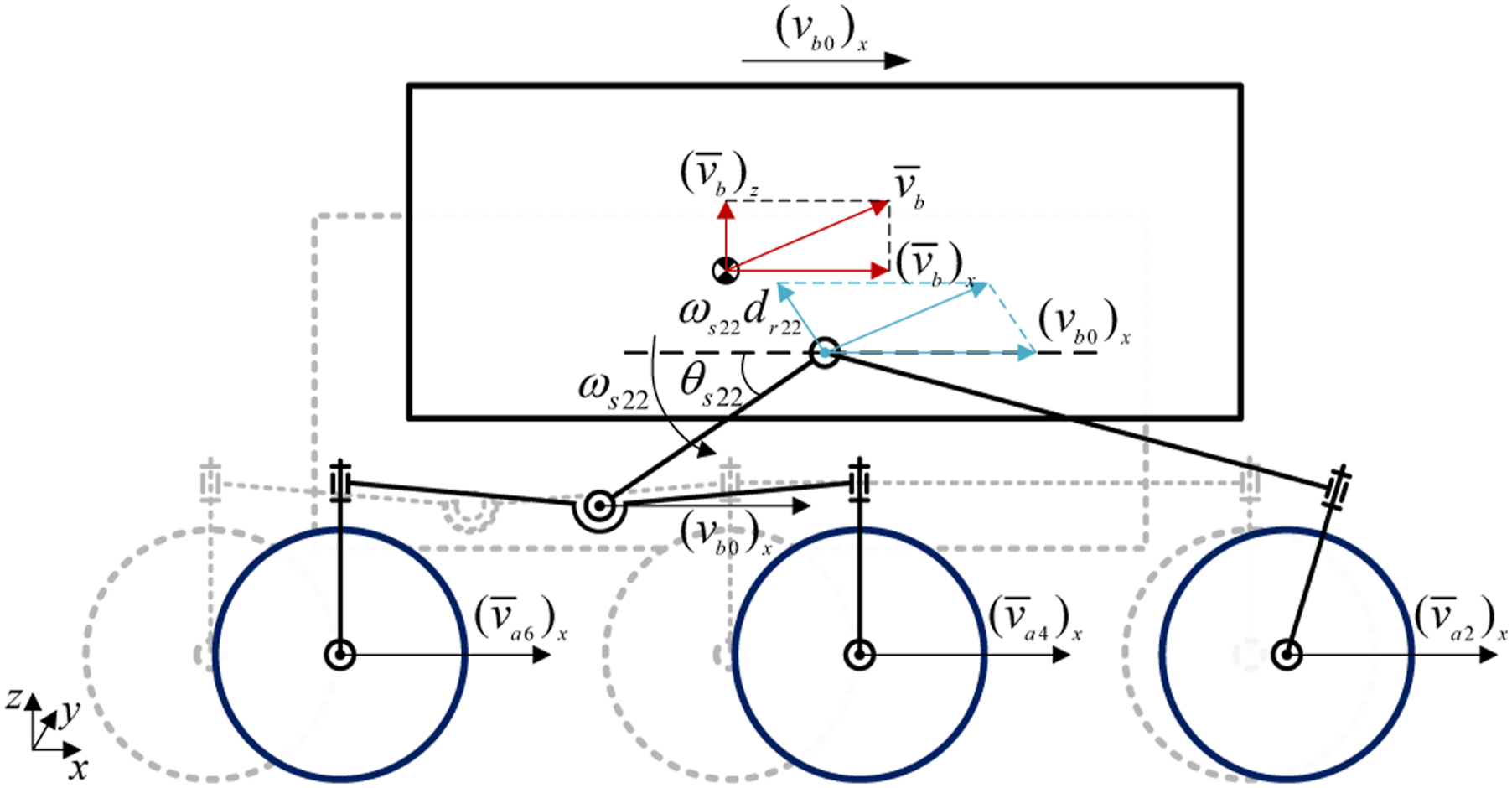

The component velocities of the hinged point of the left and right active rocker–bogies in the x- and z-directions are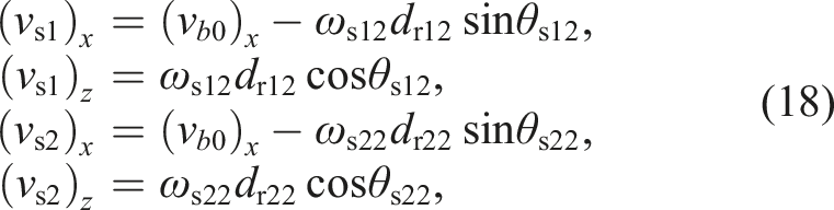

\begin{aligned} {(v_{s 1})}_{x} & = {(v_{b 0})}_{x} - ω_{s 12} d_{r 12} \sin θ_{s 12}, \\ {(v_{s 1})}_{z} & = ω_{s 12} d_{r 12} \cos θ_{s 12}, \\ {(v_{s 2})}_{x} & = {(v_{b 0})}_{x} - ω_{s 22} d_{r 22} \sin θ_{s 22}, \\ {(v_{s 2})}_{z} & = ω_{s 22} d_{r 22} \cos θ_{s 22}, \end{aligned}

(18)

where

{(v_{b 0})}_{x}

is the forward velocity of the body before it is influenced by the movement of the rocker–bogie;

{(v_{s 1})}_{x}

and

{(v_{s 1})}_{z}

(

{(v_{s 2})}_{x}

and

{(v_{s 2})}_{z}

) are the x- and z-components of the hinged point’ velocity of the left (right) active rocker–bogies.

The velocities of the CoM can be determined by utilizing the velocity superposition effect to the hinged points between the active suspension and the body box on both sides, while the suspension is in motion, as follows:

\begin{aligned} {(v_{b})}_{x} & = {(v_{b 0})}_{x} - \frac{ω_{s 12} d_{r 12} \sin θ_{s 12} + ω_{s 22} d_{r 22} \sin θ_{s 22}}{2}, \\ {(v_{b})}_{z} & = \frac{ω_{s 12} d_{r 12} \cos θ_{s 12} + ω_{s 22} d_{r 22} \cos θ_{s 22}}{2} . \end{aligned}

(19)

The angular velocities of the body box are affected by the asynchronous motion of the suspension on both sides, and their increments can be calculated as

\begin{aligned} Δ {(ω_{b})}_{x} & = \frac{ω_{s 22} d_{r 22} \cos θ_{s 22} - ω_{s 12} d_{r 12} \cos θ_{s 12}}{d_{b}}, \\ Δ {(ω_{b})}_{z} & = \frac{ω_{s 12} d_{r 12} \sin θ_{s 12} - ω_{s 22} d_{r 22} \sin θ_{s 22}}{d_{b}}, \end{aligned}

(20)

where

Δ {(ω_{b})}_{x}

is the angular velocity increment of the CoM in the x-direction of Σ_b, of which an excessive increase can cause the robot to overturn; while

Δ {(ω_{b})}_{z}

is the angular velocity increment of the CoM in the z-direction, of which an excessive increase can cause a significant change in the steering angular velocity.

To ensure stability in the motion posture of the robot body during movements, some motion constraints should be defined to minimize the roll degree of freedom (DoF) at the hinged point between the rocker–bogies and the body. In consequence, exceeding the predetermined value for the roll DoF can be caused by the asynchronous motion of the left- and right-side suspensions, as shown in Figure 9. The additional internal stress generated by asynchronous motion potentially affects the forces on the suspension joint, resulting in possible damage to mechanisms. Consequently, the asynchronous motion should be typically utilized for specific situations, such as emergency obstacle avoidance, since the steering curvature can be changed by controlling the different wheelbase lengths on both sides of the robot.

Figure 9.

Rear view of the CoM velocity of the body.

For the synchronous motion of the active suspensions, the CoM velocity can be calculated by combining the velocities of the active hinged points: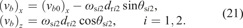

\begin{aligned} {(v_{b})}_{x} & = {(v_{b 0})}_{x} - ω_{s i 2} d_{r i 2} \sin θ_{s i 2}, \\ {(v_{b})}_{z} & = ω_{s i 2} d_{r i 2} \cos θ_{s i 2}, i = 1,2 . \end{aligned}

(21)

where i = 1, 2 represent the left and right side suspension of the robot, respectively.

4.2. Displacement of robot CoM caused by the rocker motion

As shown in the lateral view (Figure 8) and rear view (Figure 9) of the robot, the displacement changes of the robot CoM, in x- and z-directions of the hinged point between the active suspension and the body box, are induced by the motion of suspension rockers on each side, as follows: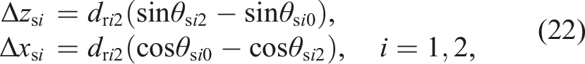

\begin{aligned} Δ z_{s i} & = d_{r i 2} (\sin θ_{s i 2} - \sin θ_{s i 0}), \\ Δ x_{s i} & = d_{r i 2} (\cos θ_{s i 0} - \cos θ_{s i 2}), i = 1,2, \end{aligned}

(22)

where d_ri1 and d_ri2 are the equivalent lengths of the front and rear sections of the ith active rocker–bogie, respectively.

Then, the displacements of the CoM in the z- and x-directions are calculated by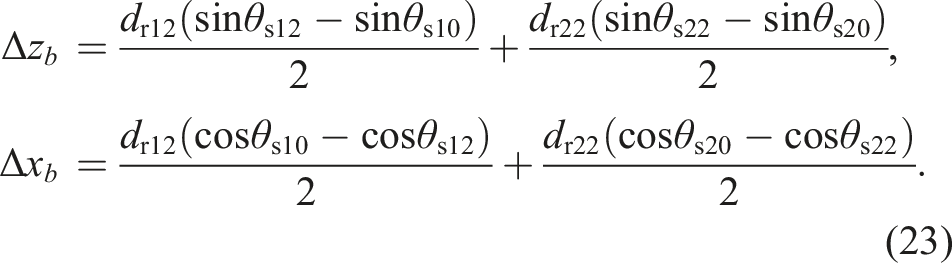

\begin{aligned} Δ z_{b} & = \frac{d_{r 12} (\sin θ_{s 12} - \sin θ_{s 10})}{2} + \frac{d_{r 22} (\sin θ_{s 22} - \sin θ_{s 20})}{2}, \\ Δ x_{b} & = \frac{d_{r 12} (\cos θ_{s 10} - \cos θ_{s 12})}{2} + \frac{d_{r 22} (\cos θ_{s 20} - \cos θ_{s 22})}{2} . \end{aligned}

(23)

The calculated displacements above should be confined within the motion limit of the SRWMR mechanism, $\underset{̲}{Δ z_{b}} \leq Δ z_{b} \leq \bar{Δ z_{b}}$ and $\underset{̲}{Δ x_{b}} \leq Δ x_{b} \leq \bar{Δ x_{b}}$ , where $\underset{̲}{Δ x_{b}}$ , $\bar{Δ x_{b}}$ , $\underset{̲}{Δ z_{b}}$ , and $\bar{Δ z_{b}}$ are the preset thresholds.

Note 1

The displacement of the CoM in the y-direction is not considered in this work, since the negligible extruding deformation between the active rocker–bogies and the body box does not significantly impact control performance.

Stability in motion posture of the robot is challenged by a substantial deviation from the initial position of the body CoM. To prevent uncertain changes in posture during suspension motion, three constraints are defined as follows:

(1) Motion Constraint #3: To avoid collision between the front and middle wheels during suspension actuation, the admissible variations of the active rocker–bogie rotation angles are bounded by equation (13). The normalized longitudinal wheelbase variation between the front and middle wheels is limited by ${\bar{η}}_{wb1}$ on the left side and by ${\bar{η}}_{wb2}$ on the right side, as follows:

\begin{aligned} η_{wb1} & = \frac{d_{r 11} (1 - \cos θ_{s 11}) + d_{r 12} (\cos θ_{s 10} - \cos θ_{s 12})}{d_{w l} - 2 r} \leq {\bar{η}}_{wb1}, \\ η_{wb2} & = \frac{d_{r 21} (1 - \cos θ_{s 21}) + d_{r 22} (\cos θ_{s 20} - \cos θ_{s 22})}{d_{w l} - 2 r} \leq {\bar{η}}_{wb2} . \end{aligned}

(24)

where θ_s10 and θ_s20 denote the initial angles of the rear sections of the left and right rocker–bogies, respectively, relative to the horizontal direction; θ_s11, θ_s12, θ_s21, and θ_s22 denote the front and rear rocker–bogie rotation angles on the corresponding sides; r denotes the wheel radius; d_wl denotes the nominal wheelbase length; and d_r11, d_r12, d_r21, and d_r22 denote the associated equivalent rocker-section lengths.

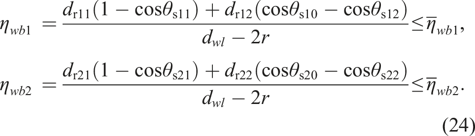
Sufficient wheel–wheel clearance is maintained by limiting the reduction in wheelbase length induced by rocker motion.

(2) Motion Constraint #4: To limit excessive body roll induced by asymmetric suspension motion, the normalized left–right chassis height asymmetry, denoted by η_r, is bounded by the threshold ${\bar{η}}_{r}$ , as follows:

\begin{aligned} η_{r} & = \frac{|d_{r 12} (\sin θ_{s 12} - \sin θ_{s 10}) - d_{r 22} (\sin θ_{s 22} - \sin θ_{s 20})|}{\max \{|d_{r 12} (\sin θ_{s 12} - \sin θ_{s 10})|, |d_{r 22} (\sin θ_{s 22} - \sin θ_{s 20})|\}} \\ \leq {\bar{η}}_{r}, \end{aligned}

(25)

where d_r12(sin θ_s12 − sin θ_s10) and d_r22(sin θ_s22 − sin θ_s20) denote the rear-rocker-induced vertical displacements on the left and right sides, respectively; their difference represents the left–right height mismatch, and the denominator normalizes the mismatch by the maximum displacement magnitude.

(3) Motion Constraint #5: To limit body yaw deviation induced by asymmetric suspension deflection during steering, the normalized left–right chassis deflection asymmetry, denoted by η_y, is bounded by the threshold ${\bar{η}}_{y}$ , as follows:

\begin{aligned} η_{y} & = \frac{|d_{r 12} (\cos θ_{s 10} - \cos θ_{s 12}) - d_{r 22} (\cos θ_{s 20} - \cos θ_{s 22})|}{\max \{|d_{r 12} (\cos θ_{s 10} - \cos θ_{s 12})|, |d_{r 22} (\cos θ_{s 20} - \cos θ_{s 22})|\}} \\ \leq {\bar{η}}_{y}, \end{aligned}

(26)

where d_r12(cos θ_s10 − cos θ_s12) and d_r22(cos θ_s20 − cos θ_s22) denote the rear-rocker-induced longitudinal deflections on the left and right sides, respectively; their difference represents the left–right deflection mismatch, and the denominator normalizes it by the maximum deflection magnitude.

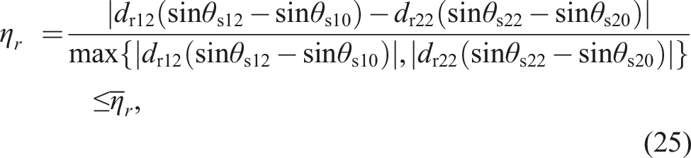
To clarify the relevant controllable parameters of robot motion, the equivalent equation of equations (24)−(26) is rewritten as follows:

C_{p i} (θ_{s 12}, θ_{s 22}) \leq 1, i = 1,2,3,4,

(27)

where C_pi(θ_s12, θ_s22) denotes the constraint expressions on the left side of the inequalities after the normalization on the right side.

The steady-state constraint of the variable CoM position is defined as follows:

γ_{p} = \min_{i = 1,2,3,4} {1 - C_{p i} (θ_{s 12}, θ_{s 22})} .

(28)

4.3. Anti body-posture instability constraints in general scenarios

To ensure the safe completion of the variable instantaneous steering radius of the wheels during movement, stability constraints for robot posture should be defined within the designed 3D differential steering kinematic model. Consequently, some motion constraints should be defined to limit the differential velocities of the body on both sides to the prescribed maximum value. First, the initial posture of the robot is set by ensuring that the support arms of all six wheels are perpendicular to the horizontal plane, with a wheelbase length d_wl between the front and middle wheels. In addition, as the suspension moves, the jointed wheels should generate additional velocity to mitigate internal force confrontation between the wheels, leading to reducing the slippage of the active-rocker-jointed wheel caused by uncoordinated velocities in the forward motion direction.

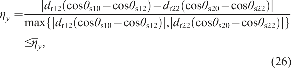
To prevent the combined velocity of the wheels on each side of the body from reaching zero during suspension motion, Motion Constraint #6 is presented to limit the angular velocity of the active rocker–bogies hinge point, using the right side as an example, as defined in equation (18).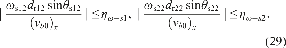

∣ \frac{ω_{s 12} d_{r 12} \sin θ_{s 12}}{{(v_{b 0})}_{x}} ∣ \leq {\bar{η}}_{ω - s 1}, ∣ \frac{ω_{s 22} d_{r 22} \sin θ_{s 22}}{{(v_{b 0})}_{x}} ∣ \leq {\bar{η}}_{ω - s 2} .

(29)

To prevent abrupt and substantial changes in the motion state of the body resulting from rocker rotation, three additional constraint rules are presented as follows:

(1) Motion Constraint #7: The forward velocity of the body cannot be substantially changed, which is evaluated by a coefficient defined as the change ratio of the velocity to the original velocity, that is, $η_{v - b x} = \frac{{(v_{b})}_{x} - {(v_{b 0})}_{x}}{{(v_{b 0})}_{x}}$ . The limitation is $∣ η_{v - b x} ∣ \leq {\bar{η}}_{v - b x}$ , and ${\bar{η}}_{v - b x}$ is the preset threshold;

(2) Motion Constraint #8: The steering angular velocity of the body cannot be changed considerably, which is evaluated by a coefficient defined as the ratio of the change in angular velocity to the original angular velocity, that is, $η_{ω - b z} = \frac{{(ω_{b})}_{z} - {(ω_{b 0})}_{z}}{{(ω_{b 0})}_{z}}$ . The limitation is $∣ η_{ω - b z} ∣ \leq {\bar{η}}_{ω - b z}$ , and ${\bar{η}}_{ω - b z}$ is the preset threshold;

(3) Motion Constraint #9: The robot cannot have a large roll angular velocity, which is evaluated by a coefficient defined as the ratio of the change in vertical velocity on both sides of the body to the original velocity, that is, $η_{v - b z} = \frac{∣ {(v_{s 2})}_{z} - {(v_{s 1})}_{z} ∣}{\max \{∣ {(v_{s 1})}_{z} ∣, ∣ {(v_{s 2})}_{z} ∣\}}$ . The limitation is $η_{v - b z} \leq {\bar{η}}_{v - b z}$ , and ${\bar{η}}_{v - b z}$ is the preset threshold.

Consequently, based on the three above rules, the inequality constraints for the angular velocity of the active rocker–bogies are as follows:

\begin{aligned} \frac{1}{r} ∣ \frac{ω_{s 12} d_{r 12} \sin θ_{s 12} + ω_{s 22} d_{r 22} \sin θ_{s 22}}{ω_{L} + ω_{R}} ∣ & \leq {\bar{η}}_{v - b x}, \\ \frac{d_{w t}}{r d_{b}} ∣ \frac{ω_{s 12} d_{r 12} \sin θ_{s 12} - ω_{s 22} d_{r 22} \sin θ_{s 22}}{- ω_{L} + ω_{R}} ∣ & \leq {\bar{η}}_{ω - b z}, \\ \frac{∣ ω_{s 22} d_{r 22} \cos θ_{s 22} - ω_{s 12} d_{r 12} \cos θ_{s 12} ∣}{\max {∣ ω_{s 12} d_{r 12} \cos θ_{s 12}} ∣, ∣ ω_{s 22} d_{r 22} \cos θ_{s 22} ∣\}} & \leq {\bar{η}}_{v - b z} . \end{aligned}

(30)

To clarify the relevant controllable parameters of robot motion, the equivalent equation of equation (30) is rewritten as follows:

C_{v i} (ω_{s 12}, ω_{s 22}, θ_{s 12}, θ_{s 22}, ω_{L}, ω_{R}) \leq 1, i = 1,2,3,

(31)

where ω_L and ω_R are the rolling angular velocities of the left- and right-side wheels, C_vi(ω_s12, ω_s22, θ_s12, θ_s22, ω_L, ω_R) are the constraint expressions on the left side of the inequalities in equation (30), after the normalization on the right side.

To further ensure the feasibility of the set value for the angular velocities ω_s12 and ω_s22 of the active rocker–bogies, the steady-state margin for velocity is defined as follows:

γ_{v} = \min_{i = 1,2,3} {1 - C_{v i} (ω_{s 12}, ω_{s 22}, θ_{s 12}, θ_{s 22}, ω_{L}, ω_{R})} .

(32)

5. Constraints for the load distribution of multi-wheels in multimode motion

To reduce the risk of body overturning, the motion constraints for the robot’s multi-wheel load distribution are defined to manage the conditions of wheel suspension during multimode motion in this section. In addition, to achieve a safe wheel lifting mode, balanced load distribution of the wheels is considered as a key controlled state in the design of the multimode control system, while the robot moves on rough or deformable terrains.

The maximum difference among the wheel load values is calculated and represented as W_diff. Additionally, the maximum difference between the highest wheel load, W_max, the lowest wheel load, W_min, and their average load, 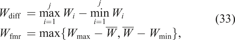$\bar{W}$ , is represented as W_fmr, as follows:

\begin{aligned} W_{diff} & = \max_{i = 1}^{j} W_{i} - \min_{i = 1}^{j} W_{i} \\ W_{fmr} & = \max {W_{max} - \bar{W}, \bar{W} - W_{min}}, \end{aligned}

(33)

where the maximum number of wheels involved in the calculation is j = 6 for HIT-MRII robot, and the j value excludes the wheels that are actively lifted off the ground.

To indicate the degree of even distribution of loads on the wheels in contact with the terrain, two Motion Constraints #10 and #11 are defined, as follows:

W_{diff} < η_{W d i ff}, W_{fmr} < η_{W a v g},

(34)

where η_Wdiff and η_Wavg are the thresholds of the difference between the maximum and minimum loads of multiple wheels and the average load of multiple wheels, in the critical unstable state of the robot, respectively.

The functions of the defined metrics W_diff and W_fmr, while the robot is in motion, are specifically as follows:

• The value of W_diff can be utilized to characterize the tendency of a wheel to lose ground contact. A suspended state of certain wheels can be indicated as the W_diff value approaches a wheel’s normal load.

• The value of W_fmr can be used to characterize the degree of load distribution among wheels. A larger value indicates a more uneven distribution, which highlights the complexity of the wheel–terrain contact.

• The values of W_fmr observed at various motion stages can be utilized to characterize the degree of pressure exerted on the wheels by the body box.

6. Threshold design for motion constraints

To enable uniform threshold enforcement across constraint metrics with different physical units and magnitudes, each motion-constraint threshold is expressed as a normalized, dimensionless index, as follows: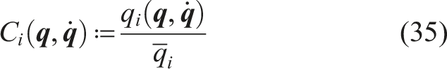

C_{i} (q, \dot{q}) ≔ \frac{q_{i} (q, \dot{q})}{{\bar{q}}_{i}}

(35)

where

q = {[σ_{w}^{⊤} q_{j}^{⊤}]}^{⊤}

is composed of the body posture σ _w and joint coordinates q _j, with its derivation

\dot{q}

;

q_{i} (q, \dot{q}) \geq 0

denotes the i-th constraint metric, normalized by the assigned bound

{\bar{q}}_{i} > 0

; and

{C_{i}}_{i = 1}^{K}

denotes the K normalized inequality constraints.

Accordingly, motion within the safety margin is indicated by $\max C_{i} (q, \dot{q}) < 1$ . Thresholds can be obtained from robot geometry and quasi-static stability considerations and are refined empirically. In specific, the nominal critical bound $q_{i}^{crit}$ is first estimated from robot geometry and quasi-static stability (e.g., allowable body-attitude and reconfiguration deviations before incipient contact loss, min W_i → 0, or excessive load concentration, large W_diff or W_fmr). A conservative margin factor κ_i ∈ (0, 1) is then applied to account for unmodeled terrain variability, actuation limits, and sensing uncertainty, as follows:

{\bar{q}}_{i} = κ_{i} q_{i}^{crit} .

(36)

Margin factor κ_i is tuned in short, mode-representative pilot trials by decreasing its nominal value until no violations are observed under the anticipated operating conditions.

Mode-dependent threshold sets were adopted since the risk profile and dominant failure mechanisms differed across motion modes. For wheel-only modes (WRM/WCM), thresholds are mainly selected to bound slip- and drift-related indices while maintaining motion continuity. For reconfiguration-enabled modes (RCLM/RCM/SWLM/DWLM), tighter limits are imposed on posture- and contact-related indices to maintain chassis-attitude stability and contact feasibility during suspension articulation. For consistent real-time enforcement in the unified IK loop, each mode is assigned a threshold vector $Θ_{m} = {{\bar{q}}_{k}}_{k = 1}^{N_{c, m}}$ , where N_c,m ≤ K denotes the number of constraints enforced in the given motion mode.

Thresholds are set from geometric bounds with safety margins, and $q_{i}^{crit}$ and κ_i can be recalibrated for other types of robots or terrains without changing the designed constraint structure.

7. Model-based control system design of multimode motion

A diagram of the designed model-based control system of the robot for multimode motion is shown in Figure 10. The control system consists of three parts: the built 3D kinematic model (using the inverse of equation (7)), state observer of motion constraints (using the defined Motion Constraints #1 ∼ #11), and a decision-making strategy. In addition, the posture of the robot’s body is measured by the OptiTrack system during movements.

Figure 10.

Model-based control system of multimode motion.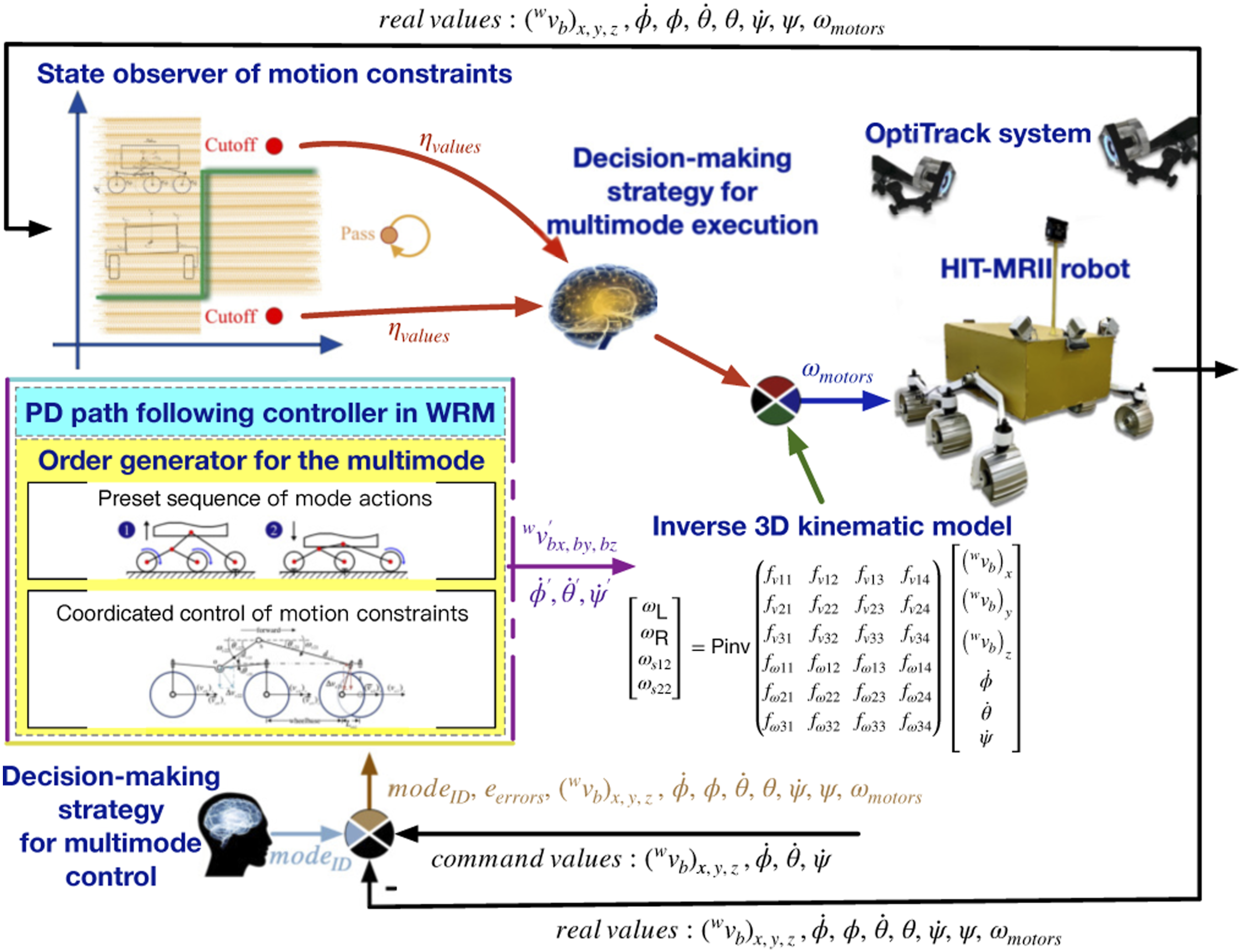

The value of e_errors is defined as the difference between command values and real values, as follows: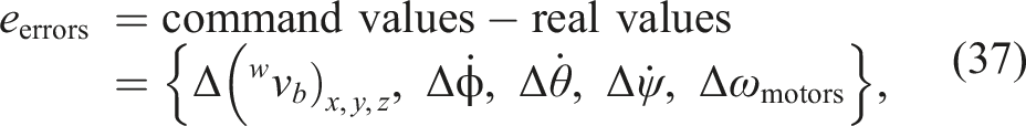

\begin{aligned} e_{errors} & = command values - real values \\ = \{Δ {({}^{w}v_{b})}_{x, y, z}, Δ \dot{ϕ}, Δ \dot{θ}, Δ \dot{ψ}, Δ ω_{motors}\}, \end{aligned}

(37)

where Δω_motors represents the difference value of the angular velocity for the active suspension rockers, the wheel rolling, and the wheel heading.

To validate the practicability of both the built model and all the presented motion constraints for control, a simple overall strategy of decision-making for multimode execution is designed in this work. Specifically, two control strategies of the optimal motion mode were developed and executed: one is for manual operations, and the other is for automatic operations. For the manual operations, obstacles were placed on a straight path, and their sizes were known to the control system. When the distance between the robot and an obstacle, as observed by the OptiTrack system, fell within a preset threshold, the corresponding mode was automatically activated by the proposed model-based control method.

For the automatic operations, when the control indicators reach the predefined threshold of the established motion constraints, the robot’s motion was halted, and a command reminder was displayed in a window message to the operator. If feedback from the operator was not received within a specified period of time, the current motion mode would be executed in a reverse order until the robot returned to its initial state. Upon receiving feedback, the current action would be terminated by the designed control system, and the subsequent action in this mode would be further performed until the mode was achieved or the next reminder was received. Notably, the robot was forcibly controlled to return to the initial state if two reminders were generated within a single mode. In Figure 10, η_values consists of the thresholds of the defined motion constraints.

Remark 2

For motion modes of the chassis lifting and wheel lifting of the robot, the control command is determined based on the established 3D model and the multi-joint coordinated motion constraints. For instance, in the RCLM, the commanded velocity to lift the chassis is calculated using the model, while the wheel velocity, coordinated with the suspension, is determined based on the corresponding Motion Constraint #2.

7.1. Quasi-static stability interpretation of constraint-based inverse kinematics control

For a low-speed robot, each motion mode can be approximated as a sequence of quasi-static equilibria (Lyu et al., 2023). Quasi-static stability is characterized by safety margins on body posture (motion constraints, MCs #4 and #5), commanded velocity (MCs #6–#9), and contact-force maintenance (MCs #10 and #11) under terrain disturbances and small inertial effects. For each motion mode, an admissible set Ω_m is defined by the normalized inequality constraints in equation (35), using the mode-specific threshold vector Θ_m with N_c,m enforced constraints.

Ω_{m} ≔ \{(q, \dot{q}) | C_{k, m} (q, \dot{q}; Θ_{m}) \leq 1, k = 1, \dots, N_{c, m}\} .

(38)

A commanded posture can be regarded as feasible when quasi-static force–moment balance about the body CoM (as MCs #4–#5) is satisfied by the wheel–terrain contact forces (Iagnemma and Dubowsky, 2004a), as follows:

\sum_{i = 1}^{N} f_{i} + m g \approx 0, \sum_{i = 1}^{N} {[p_{i} - p_{c}]}_{\times} f_{i} \approx 0,

(39)

where N is the number of contacts; f _i is the contact force at wheel i; m is the robot mass; g is gravity; p _i is the i-th contact position; and p _c is the CoM position.

To maintain a safety margin against the Coulomb friction feasibility bound in equation (40), anti-slip and velocity-smoothing constraints (as MCs #6–#9) are imposed to limit lateral slip and inter-wheel velocity mismatch. These limitations can be introduced as kinematic approximations that reduce tangential interaction demand associated with the commanded motion at each wheel–terrain contact (Iagnemma and Dubowsky, 2004b).

‖ f_{t, i} ‖ \leq μ_{i} W_{i},

(40)

where W_i is the normal load, f _t,i is the tangential force at wheel–terrain contact i, and μ_i is the friction coefficient.

Tip-over risk is increased when the normal load is redistributed toward a subset of wheels (as MCs #10–#11). Incipient contact loss is indicated as min_iW_i approaches zero, whereas large W_diff or W_fmr indicates load concentration that typically precedes tip-over under the quasi-static balance in equation (39).

The closed-loop inverse-kinematics control is designed as constraint-saturated feedback. At each control cycle, the nominal command ${\dot{q}}_{0}$ is utilized when it satisfies all constraints; otherwise, ${\dot{q}}^{⋆}$ is calculated as the Euclidean projection of ${\dot{q}}_{0}$ onto the feasible set evaluated at the measured configuration q , as follows:

\begin{aligned} {\dot{q}}^{⋆} = \arg \min_{\dot{q}} ‖ \dot{q} - {\dot{q}}_{0} ‖^{2} \\ s.t. C_{k} (q, \dot{q}) \leq 1, k = 1, \dots, N_{c, m} . \end{aligned}

(41)

When monitored margins fall below preset thresholds due to sustained unloading or friction-limit operation at one or more contacts, motion execution is halted, and mode-transition or rollback is initiated by the supervisory logic to avoid operation near instability. If the projection in equation (41) is feasible, the executed command remains in Ω, and constraint satisfaction is maintained during mode execution and transitions. Equation (41) is solved at each control cycle as a constrained least-squares problem with N_c,m inequality constraints, enabling real-time enforcement of the constraints.

Remark 3

MC #1 is imposed as a mode-level contact precondition, and MCs #2 and #3 are enforced as wheel–suspension velocity coordination and wheel–wheel clearance constraints. As feasibility prerequisites, they are not considered as stability-margin indicators under disturbances.

8. Experiments

One experimental setup is used to validate the proposed inverse kinematics control (IKC) method, a self-reconfigurable wheeled mobile robot with actively and passively articulated suspensions and six wheels, HIT-MRII, as shown in Figure 11. All experimental tasks of the HIT-MRII robot were conducted at a Mars surface simulation site.

Figure 11.

Self-reconfigurable wheeled mobile robot with actively and passively articulated suspensions and six wheels: HIT-MRII.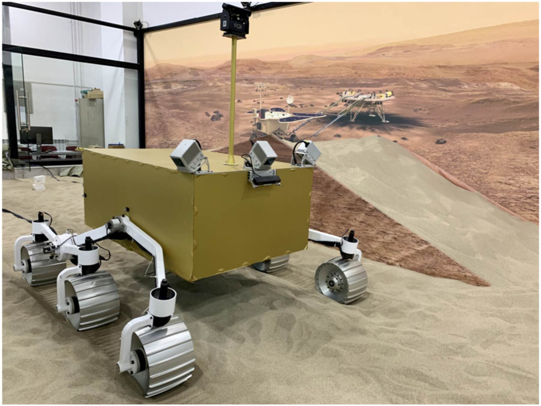

8.1. Experimental setup

The configuration of HIT-MRII, as shown in Figure 11(a), is similarly aligned with the mechanical structure of the robot introduced in (Zheng et al., 2018). HIT-MRII is equipped with an industrial computer (BECKHOFF C6930-0060) situated within the body box, 12 brushed DC motors (FAULHABER 3056K024B-K1838) in the wheels, six incremental encoders (FAULHABER IE3-1024L), eight absolute encoders (RWARE 232RTU1224M6), three binocular cameras (ZED2), three LIDARs (Livox Horizon), and six 6-axis Force/Torque (F/T) sensors (SRI M3616C). Measurement ranges of the F/T sensors are as follows: F_x/F_y are 2700 N, F_z is 4000 N, M_x is 180.0 N⋅m, M_y is 180.0 N⋅m, and M_z is 144 N⋅m, of which accuracy is 0.04%, 0.02%, 0.06%, 0.13%, and 0.03% F.S., respectively.

Each wheel is equipped with a linear motor with an incremental encoder, and a steering motor with an absolute encoder in HIT-MRII. For the suspension systems on each side of the body, active driving capabilities are incorporated into the active suspension by installing a motor (FAULHABER 4490K024B-K1155), an incremental encoder, and a single-turn absolute encoder (RE38-Z06G-S1200-SG3) at the hinge point between the suspension and body box. An angle sensor (P4500) is mounted at the hinge point between the passive suspension and the rear section of the active suspension rockers on each side of the body. In addition, the connection between the actively and passively articulated suspension rockers is facilitated by an electromagnetic clutch (STEKI ETC-500-50-14-NF). Two cameras are installed on the top and front of the body box, and one camera is mounted on the mast of the body box. Furthermore, the motion posture of the robot body and traveling velocity are measured by a motion capture system (OptiTrack Prime 22 with the accuracy of position ±0.15 mm and attitude $\leq 0.5 °$ ).

Moreover, the physical property parameters of the planetary soil simulants in experiments (Yang et al., 2022) are the pressure-sinkage modules, k_c and k_φ, sinkage exponent n, soil cohesion c, internal friction angle of the soil φ, and shearing deformation modulus K, as shown in Table 4.

Table 4.

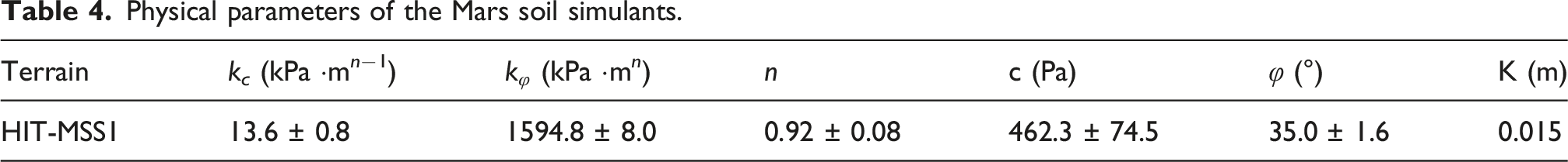
Physical parameters of the Mars soil simulants.

Terrain	k_c (kPa ⋅mⁿ⁻¹)	k_φ (kPa ⋅mⁿ)	n	c (Pa)	φ (°)	K (m)
HIT-MSS1	13.6 ± 0.8	1594.8 ± 8.0	0.92 ± 0.08	462.3 ± 74.5	35.0 ± 1.6	0.015

8.2. Experimental parameter settings and tasks

In the operating system of the industrial computer, the sampling period was set to T_s = 0.01 s. The robot model parameters (equation (4)) were set to r = 150 mm, d_wt = 1304 mm, and d_b = 830 mm; the equivalent lengths of the articulated rocker arms were set to d_r21 = 775 mm and d_r22 = 390.7 mm. The initial wheelbase length (equation (24)) was set to d_wl = 1550 mm. The posture angles ϕ, θ, and ψ were obtained from real-time sensor measurements. The ratio between the angular velocities of the front and rear sections of the active rocker–bogie (equation (12)) was set to z = 1/2.2. Furthermore, the thresholds for equation (23) were set to $\underset{̲}{Δ x_{b}} = - 10$ mm, $\bar{Δ x_{b}} = 10$ mm, $\underset{̲}{Δ z_{b}} = - 10$ mm, and $\bar{Δ z_{b}} = 10$ mm. Other defined thresholds are set differently in different motion modes.

Remark 4

The maximum movable distance and velocity of the robot’s joints vary across different terrain environments, depending on the interaction state between the wheel and terrain. In this work, the maximum mobility performance for each action in different modes was pre-tested on the soil terrains, and the obtained data were used as the basis for setting the defined thresholds of the presented constraints.

The validation of the 3D straight-line kinematic model and the presented motion constraints is the objective of the first seven tasks. In Task 1, the regular Wheel Rolling Mode (WRM) is implemented by the HIT-MRII on flat, loose, and sandy terrain. Task 2 involves the utilization of the Wheel Crabbing Mode (WCM) by the HIT-MRII on flat, loose, and sandy terrain with obstacles. Task 3 involves an examination of the HIT-MRII in the Robot Chassis Lifting Mode (RCLM) on flat, loose, and sandy terrain with two different height obstacles. Tasks 4 and 5 focus on the HIT-MRII executing the Robot Creeping Mode (RCM) on loose sandy terrain, featuring flat and upslope areas, respectively. In Task 6, the Single Wheel Lifting Mode (SWLM) is performed by the HIT-MRII on flat, loose, and sandy terrain to overcome a brick wall obstacle. Finally, Task 7 involves the testing of the HIT-MRII in the Double Wheel Lifting Mode (DWLM) to climb a staircase-type terrain. This specific set of tasks ensures a thorough evaluation of the robot’s capabilities in multimode motion on challenging terrains, including scenarios with obstacles.

Furthermore, the next seven experimental tasks were designed to demonstrate enhanced mobility across different motion modes. In Task 8, the effect of speed stage variations, ranging from 5 mm/s to 25 mm/s, on the energy efficiency of the WRM was mainly assessed by controlling the robot to follow a straight-line path. In Task 9, the steering agility of WRM (Ackermann) and WCM was compared by directing the robot to reach position B from position A via a curved path with a 45-degree turn and a straight path, respectively. In Task 10, the effect of normal force variations of the wheels was mainly validated on RCLM performance in traveling velocity, by raising the robot’s chassis to four different heights from 150 mm to 550 mm. In Task 11, the traction efficiency of the RCM and WRM was mainly compared by commanding the robot to traverse a sloped soil terrain with a 15^◦ incline from flat terrain. Task 12 mainly focused on the variation in the drawbar pull coefficient of the wheels. Single-wheel and double-wheel configurations were lifted to different heights ranging from 100 mm to 200 mm. In Task 13, the drawbar pull coefficient was further analyzed by lifting wheels at various positions on the robot—the front, middle, and rear wheels—at heights up to 200 mm. Additionally, in Task 14, the mobility for obstacle overcoming of the WRM, WCM, RCLM, and SWLM was compared by multiple metrics. To illustrate both the general results and detailed variation trends in the data, each curve was generated by averaging the results of three experimental trials, in addition to the force curves shown in the figures.

Moreover, to validate the motion performance of the built 3D steering kinematics model of differential velocity, Task 15 was performed by changing the wheelbase length between the front and middle wheels.

Remark 5

For the conducted experiments, the Motion Constraint #1 was utilized to preset the sequential actions of the multi-joints in the wheel-lifting mode. The kinematics model of the robot and Motion Constraint #2 were employed to generate the control commands for the motors during multimode motion. In addition, to achieve the maximum motion performance of each mode, the defined thresholds in Motion Constraints #3 to #11 were used as a measure to monitor the stability of the body posture during motion, and ensure safety.

8.3. Real-time control execution

To satisfy safety-critical timing requirements, real-time optimal-control workloads have been reported to require update rates of 100−400 Hz (Dong et al., 2025). The real-time control feasibility is supported by solving the constrained least-squares projection in equation (41) within each 10 ms Ethernet cycle on the onboard industrial PC (Beckhoff Automation GmbH & Co. KG, 2025).

Within each cycle, motor encoders were sampled to obtain wheel and suspension joint states, wheel–terrain contact forces were measured by six-axis F/T sensors at each wheel, and body pose was provided by an external motion capture system. The measurements were time-stamped, synchronized, and supplied to the controller. Joint-velocity references were computed and transmitted to the wheel and suspension drives within the cycle, establishing a low-latency sensing–actuation loop for real-time motion control.

8.4. Results of multimode motion performance

To evaluate the multimode motion performance of the robot, a general formula for calculating the relative error δ_value of a certain indicator is defined as follows: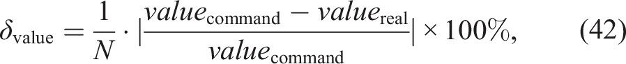

\begin{matrix} δ_{value} = \frac{1}{N} \cdot | \frac{v a l u e_{command} - v a l u e_{real}}{v a l u e_{command}} | \times 100 %, \end{matrix}

(42)

where N denotes the number of cycles of a motion mode, value_command denotes a command value, and value_real denotes a real value.

In Task 1, the HIT-MRII utilized the WRM mode, with a specified forward velocity of 25 mm/s, as shown in Figure 12(a). The command moving time is set to 153.82 s, and the real moving time is 182.92 s. Furthermore, the error in the motion time of the robot, denoted as δ_time, is calculated to be 18.92% using equation (42) (with parameter N = 1). This result demonstrates a considerable level of wheel slippage on sandy and loose terrains, resulting in a substantial decrease in the overall motion efficiency. Moreover, the WRM is a regular mode that does not require kinematic constraints to ensure motion safety, since it involves no self-reconfiguration actions.

Figure 12.

Multimode locomotion of HIT-MRII robot. WRM and WCM are wheel-only modes, and RCLM, RCM, SWLM, and DWLM involve suspension rocker-arm reconfiguration.

In Task 2, the robot encountered a brick wall during its forward motion (named period A, the WRM mode is active). All wheels performed an in-place clockwise rotation of 90°, followed by driving the wheels until the robot’s body cleared the bricks. Subsequently, the wheels rotated counterclockwise by 90° (named period B, the WCM mode is active), allowing the robot to move in a straight line until it encountered the other obstacles (named period C, the WRM mode is active). All wheels then rotated counterclockwise by 90°, driving the wheels until the robot cleared the rocks. Finally, with all wheels rotating clockwise by 90° (named period D, the WCM mode is active), the robot continued to drive the wheels until reaching the destination (named period E, the WRM mode is active), as shown in Figure 12(b).

Moreover, in periods A, C, and E, the command moving distance of the summed movements is 6422.75 mm, and the corresponding real distance is 4727.74 mm. The error in the motion distance, denoted as δ_distance, is calculated to be 26.39% using equation (42) (with parameter N = 1). Moreover, in periods B and D, the command moving distance of the summed movements is 1363.75 mm, and the corresponding real distance is 978.18 mm. The error in the motion distance is calculated to be 28.27% using equation (42) (with parameter N = 1). Furthermore, the WCM mode is capable of changing the forward direction of the body to any degree (without the terrain space cost of changing toward a degree in regular steering). Consequently, the traverse ability of HIT-MRII can be enhanced by utilizing WCM in narrow environments or on terrain with densely distributed obstacles. In addition, as with the WRM mode, the WCM mode does not require kinematic constraints to ensure motion safety.

In Task 3, as shown in Figure 12(c), the initial ground clearance of the HIT-MRII robot chassis is set to 250 mm. While moving straight in the WRM process, the robot comes to a stop when it encounters a pile of stones at a height of 300 mm in front of the robot. RCLM mode is then utilized, and the chassis is lifted to 330 mm before the robot continues to move in WRM. In sequence, facing a pile of rocks at a height of 450 mm in the forward direction, the body continues moving. Simultaneously, the RCLM is employed to lift the chassis height to 480 mm, allowing the robot to traverse the obstacle using WRM. Finally, the RCLM is utilized to lower the ground clearance back to the initial 250 mm after the robot moves away from the obstacles.

Moreover, based on the defined Motion Constraint (MC) #2, the variation of velocities of the front wheels was generated to coordinate the angular velocities of the active rocker–bogies. In this task, the velocity of the robot chassis is set at 3.6 mm/s during the lifting processes of RCLM. The variation of the velocities of the front wheels is set to −5.3 mm/s, within the desired range of velocities −7.2 ∼ −4.9 mm/s. On the other hand, the front wheels are set to 5.3 mm/s in the motion process of descending the robot chassis, within the desired range of −7.0 ∼ 4.4 mm/s. The generation velocities of the wheels are shown in Figure 13(a). Referring to the calculating method of wheel slip by observing the wheel imprint (Li et al., 2020), the wheel slip is close to zero, resulting from the introduced MC #2, as shown in the Experimental video (Appendix C section).

Figure 13.

Results of the Motion Constraints in Task 3. *The time point for switching between different actions is represented by the red triangle symbols.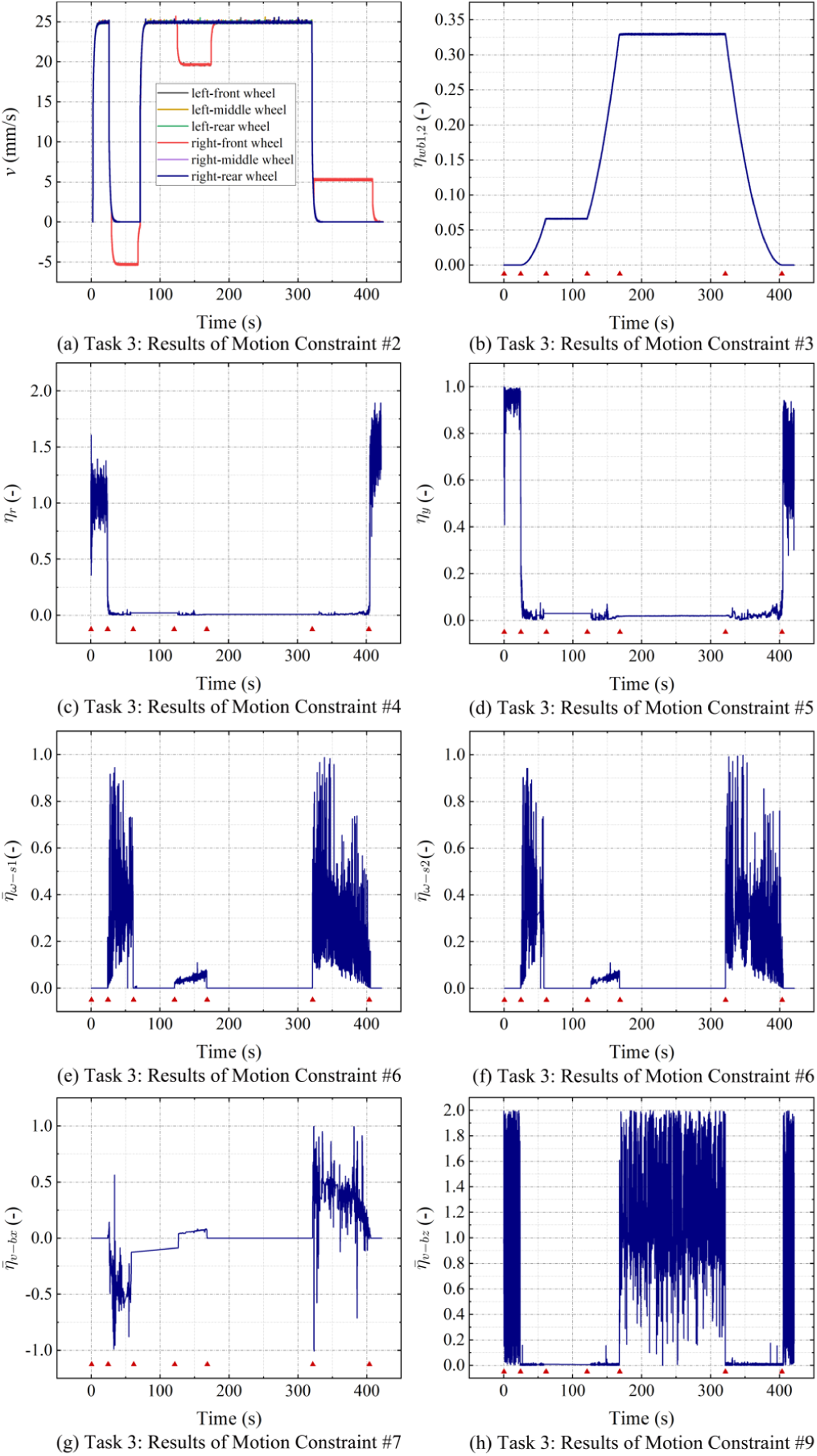

Note 2

The MC #2 has been utilized in tracking complex motion trajectories in another work (Qi et al., 2025b), and its effectiveness in coordinating the velocity between the active rockers and driving wheels has been more thoroughly validated.

Furthermore, the result of η_wb1,2 in MC #3 is shown in Figure 13(b). The maximum value of η_wb1,2 is 0.326, which is lower than the preset threshold ${\bar{η}}_{wb1,2}$ = 0.7, proving the motion process without the risk of wheel collision in this task. As shown in Figure 13(c) and (d), the results of η_r and η_y in MCs #4 and #5, remain around zero besides the begin and end periods of RCLM, which is lower than the preset thresholds, ${\bar{η}}_{r}$ = 2 and ${\bar{η}}_{y}$ = 0.7. It indicates a low risk of rollover in this task, while the value has a large changing range from 1 to 1.75 in the WRM mode. According to the designed motion process for this task, the combination of control in WRM and RCLM is only utilized in the second chassis-lifting process. Consequently, the results of the first and third chassis-lifting processes are accomplished without the involvement of MC #6, whose values are close to the threshold ${\bar{η}}_{ω - s 1, s 2} = 1$ . As shown in Figures 13(e) and (f), the values of η_ω−s1 and η_ω−s2 are around 0.05 in the second chassis-lifting process, which indicates that there is a low risk that the combined velocity of the wheels on each side of the body would reach zero. Furthermore, the result η_v−bx of MC #7 proves that the change in forward motion velocity of the robot caused by suspension movement is small in the case of the combination control of WRM and RCLM modes, and lower than the preset threshold value ${\bar{η}}_{v - b x}$ = 0.7. In contrast, the η_v−bx value is large in the case of RCLM control, which indicates that the suspension motion has a substantial effect on the velocity of the robot. Finally, the result η_v−bz of MC #9 is small in the motion period of RCLM and the combined WRM and RCLM (it is lower than the threshold ${\bar{η}}_{v - b z}$ = 0.7), but it is more significant in the motion period of WRM. Consequently, the risk of rollover in RCLM motion can be neglected in such a motion.

In Task 4, as shown in Figure 12(d), when all wheels are totally sunk in sandy soil, the RCM mode is utilized by HIT-MRII for escaping the wheels from sinking. Within the control of RCM, the RCLM is repeatedly executed in a sequence. In this task, the RCM is utilized by HIT-MRII, and RCLM is activated five times in order to successfully traverse out of the challenging terrain. To further explore the effect of wheel sinking conditions on movements, the error sequences between command and actual time spent in the lifting and descending phases of this mode are recorded as {0.12, 0.07, 0.75, 1.24, 0.43} seconds, and {0.22, 0.51, 0.21, 0.27, 0.69} seconds, respectively. It shows no significant motion resistance due to the soil to the suspension system. Moreover, the error sequence between the commanded and the actually lifted height of the chassis for the five cycles is recorded as {14.03, 32.7, 31.21, 23.37, 26.76} mm. The irregular variation of the values is caused by the complex wheel–terrain contact conditions during the robot’s process of escaping from sinking, since the soil mounds created around different wheels during their extrication will resist the escaping from sinking of other wheels or their movement. The errors of execution time and lifted height of RCM mode control are 0.89 % and 17.74 %, respectively, calculated by equation (42) (with parameter N = 10). These results demonstrate that the wheel–terrain interaction condition has a small effect on execution time, but a large effect on the control of the height of the robot chassis.

Moreover, MC #2 is utilized in this task, and the velocities of the middle and rear wheels are set to 7.0 mm/s within the desired range of 6.8 ∼ 7.1 mm/s when the command velocity of the robot chassis is 3.6 mm/s. In consequence, the velocities of the front wheels are set to 7.0 mm/s, under the same range of the command velocity. Figure 14(a) shows the maximum value η_wb1,2 of MCs #3 is 0.15, which is lower than the corresponding threshold ${\bar{η}}_{wb1,2} =$ 0.7, and indicates the low risk of the collision of wheels in this task.

Figure 14.

Results of the Motion Constraints in Tasks 4 and 5. *The time point for switching between different actions is represented by the red triangle symbols.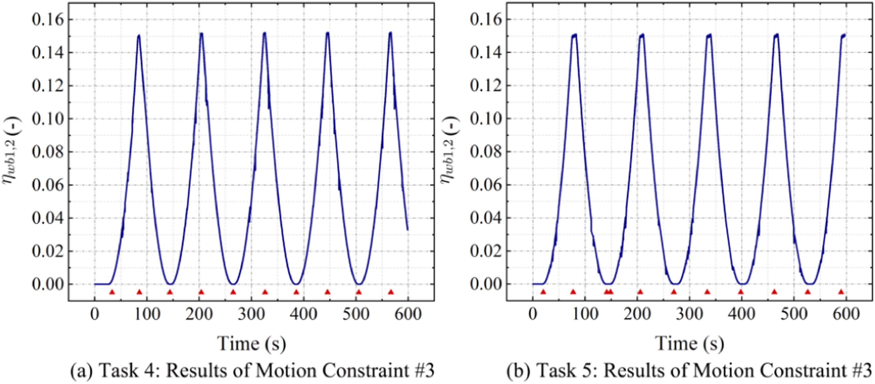

In Task 5, the RCM is utilized by HIT-MRII to climb upslope sandy terrain with 10°, as shown in Figure 12(e). Due to the configuration of the terrain and characteristics of Mars soil simulant, the WRM mode cannot provide enough driving force to move along the slope. The control design of RCM is the same as the one used in Task 4. The WRM mode is initially utilized by HIT-MRII to move on the slope until the climbing efficiency falls below the predetermined threshold (10%). Next, the RCM mode is activated, and within it, the RCLM is repetitively executed four times. Moreover, in the period of WRM control, the command moving time is 17.47 s, and the real moving time is 18.21 s. Consequently, the percentage of the time when wheels are blocked equals 4.24%. This is due to the resistance of the terrain regarding wheel rotation and it is calculated by equation (42) (with parameter N = 1). Moreover, the command moving distance of WRM is 437.75 mm, and the traveled distance is 43.65 mm. In consequence, the distance error is 90.03 %, calculated by equation (42) (with parameter N = 1). In the lifting and descending phases of RCM control, the error sequences between command and actual spent time are {0.84, 0.09, 0.02, 1.05, 0.46} seconds and {0.92, 1.59, 0.19, 0.35} seconds, respectively. The corresponding error sequences between command and real moving distances are {51.34, 49.22, 53.71, 56.51, 59.81} mm and {43.83, 44.88, 50.54, 57.29} mm, respectively. In consequence, the blocked time is 1.07%, due to the resistance from the sandy terrain to the rotation of the active rocker–bogies. The distance error of the RCM is 24.36%, calculated by equation (42) (with parameter N = 9). In this task, the total climbed height of the robot is 187.15 mm, and the corresponding forward distance is 168.90 mm. Compared to the result of WRM, the climbing ability of HIT-MRII with RCM mode is increased by 72.94 %. Moreover, the results η_wb1,2 of MC #3 is shown in Figure 14(b), and the threshold setting and the consequent analysis of MCs #2 and #3 are the same as that of Task 4.

In Task 6, the SWLM mode is utilized by HIT-MRII to lift the right wheels in sequence to overcome a pile of bricks with a height of 150 mm, as shown in Figure 12(f). Initially, the robot’s chassis is lifted to align the CoM at the rear part of the robot body in the motion plane. Then, after the right-side clutch between the actively and passively articulated suspensions is engaged, the angle of active suspension rocker–bogies, denoted as θ_s2 = 180^◦ − θ_s21 − θ_s22, is controlled to reduce and consequently lift the front wheel 180 mm above the ground. The robot moves forward to make the front wheel traverse the brick using the WRM mode. Then, reversing these steps restores the robot to its initial state. Furthermore, to lift the right and middle wheel, after the right-side clutch is engaged, the θ_s2 is controlled to reduce and consequently lift the middle wheel 180 mm. The WRM mode is utilized for forward movements, allowing the middle wheel to traverse the bricks. Then, reversing these steps returns the robot to its initial state. Next, for the rear wheel, the ground clearance of the robot is decreased to align the CoM at the front part of the robot body in the motion plane. The right-side clutch is engaged, and then the θ_s2 is increased to lift the rear wheel 15 mm above the ground. After the robot moves forward to traverse the brick using the WRM mode, the control process is reversed to return to the initial state.

MC #1 has been taken into account in the design process of Task 6, where N_w = 1. In addition, with the consideration of MC #2, the front wheel variation is set to 7 mm/s, falling within the constraint range of −7.1 ∼ −6.6 mm/s when the lifting velocity of the robot chassis is set to 3.6 mm/s. During the front-wheel lifting phase, the velocities of the middle and rear wheels are set to 6.8 mm/s, aligning with the desired range of 6.6 ∼ 6.9 mm/s, corresponding to a chassis-lifting velocity of 6.8 mm/s. Similarly, during the lowering process, the velocities of the wheels and suspensions are maintained at the same values as in the lifting process. Furthermore, in the lifting action of middle wheels, the variation velocities of the front and rear wheels are set to −2.3 mm/s and 4.8 mm/s, respectively, within the constraint range of summed velocities ranging from 6.7 to 7.1 mm/s. In contrast, during the middle wheel lowering action, the velocity variations for the front and rear wheels are 2.9 mm/s and −3.8 mm/s, respectively, falling within the constraint velocity range 6.7 ∼ 6.8 mm/s. In the rear wheel lifting action, the front wheel velocity variation is set to 3.1 mm/s, and that of the middle and rear wheels is −3.9 mm/s. The sum of their absolute values falls within the constraint value of 7.1 mm/s. Correspondingly, the velocities of the wheels and suspensions are maintained at the same values during the corresponding lowering process as those set in the lifting process. Moreover, as shown in Figure 15(a), where the time point for switching between different actions is represented by the red triangle symbols, the maximum of η_wb2 is around 0.26 smaller than its threshold ${\bar{η}}_{wb2} =$ 0.7, and the consequent risk of wheel collision (MC #3) is low. However, the risks of the robot rollover and its additional yaw angle are higher than in other tasks, resulting in asymmetric motion on both sides of the robot suspensions, as shown in Figures 15(b) and (c), respectively. According to the sensor data, the major risks occur in the WRM mode after the actions of the SWLM mode. In the control process, the parameters set for this task are almost at their maximum values, such as the lifting height of the wheel in such terrain and the moving velocity in WRM after the actions of the SWLM mode, contributing to the defined motion range of multi-joints in MCs. In addition, the results η_r and η_y of MCs #4 and #5 are large but within their thresholds of ${\bar{η}}_{r} = 2$ and ${\bar{η}}_{y} = 1$ .

Figure 15.

Results of the Motion Constraints in Tasks 6 and 7.

Furthermore, as shown in Figures 15(d) and (e), the value of η_ω−s1 for MC #6 almost remains unchanged in this task, and η_ω−s2 is available since only the wheels on the right side of the body were lifted. According to the data, the value of η_ω−s2 is large during motion (but it is lower than its threshold ${\bar{η}}_{ω - s 2}$ = 1), as the robot is in the in-situ state most of the time, resulting in the SWLM and WRM not being compounded in the control process. Moreover, the additional velocity of the robot caused by the motion of the suspension in the forward direction is large in the SWLM control. This is the result of η_v−bx of MC #7 that is similar to that of Task 3, as shown in Figure 15(f). Furthermore, the additional roll angular velocity η_v−bz of MC #9 is large in the control process of SWLM, which is close to the thresholds ${\bar{η}}_{v - b z} =$ 2, as shown in Figure 15(g). The reason is the same as one discussed in the analysis of MC #4 in this task.

Moreover, for the interaction between the wheels and the terrain, the average wheel load was measured to be approximately 380 N when the robot was in its initial nominal state. During Task 6, the maximum lifted heights of the wheels were achieved. The majority of the wheel load was supported by the middle wheels when the front or rear wheel was lifted, while the rear or front wheels were nearly suspended in the air, respectively. Additionally, the maximum differences in wheel load among the wheels, denoted as W_diff, were measured as 826 N and 1050 N for the two respective states. Furthermore, the front and rear wheels almost equally shared the additional wheel loads when the middle wheel was lifted, resulting in a W_diff average value of approximately 250 N. The variation trend of W_diff is observed to be similar to the maximum difference, W_fmr, between multiple wheels’ loads and their average values. However, the value of W_fmr is significantly smaller than that of W_diff in cases where some wheels were lifted off the terrain, as illustrated in Figure 15(h). Furthermore, in the scenario where the right front wheel is lifted, the average difference between W_diff and W_fmr is 294 N, whereas during the subsequent preparation for lifting the middle wheel, the average difference value decreases to 61 N. This indicates that the variation relation between W_diff and W_fmr is non-proportional. Additionally, a significant value of W_diff corresponds to situations where some wheels are nearly suspended in the air, particularly under a high level of the value in W_fmr. As a result, W_fmr is more critical for assessing the safety of the robot’s motion under non-wheel-lifting operations in the conducted experiments, while W_diff becomes particularly significant during partial wheel-lifting operations. To ensure the safety of the SWLM motion, thresholds of MCs #10 and #11 were set for W_fmr and W_diff. Specifically, the value of η_Wdiff1 was set to 1100 N for cases where the robot had actively lifted wheels, and that of η_Wavg1 was set to 700 N.

In Task 7, to climb a staircase terrain, the wheels at the same positions on both sides of the robot are lifted in sequence, as shown in Figure 12(g). The design process of the control in DWLM mode is the same as that of SWLM mode. In addition, the MC #1 is set to N_w = 2, and the set of MC #2 is the same as in Task 6. Moreover, the result η_wb1,2 of MC #3 demonstrates no risk of collision of wheels (the corresponding threshold is ${\bar{η}}_{wb1,2} =$ 0.7), as shown in Figure 15(i). The velocities on both sides of the robot box are close to zero in DWLM, which is the same as that of SWLM. Consequently, the results η_ω−s1 and η_ω−s2 of MC #6 are large in control phases of DWLM, but under the corresponding threshold ${\bar{η}}_{ω - s 1, s 2} = 2$ , as shown in Figures 15(j) and (k). The result η_v−bx of MC #7 is larger than in other tasks, due to the fact that the simultaneous motion of the suspensions on both sides of the robot has a large effect on the velocities of the robot in the forward-moving direction. The value ∣η_v−bx∣ is closed to the preset threshold ${\bar{η}}_{v - b x} = 1$ , while it has dramatic changes in the control phases of the DWLM mode, as shown in Figure 15(l). In addition, the absolute value of η_v−bx larger than one indicates a backward movement in the CoM position of the robot body. The maximum motion ability for DWLM in the HIT-MRII robot is presented by this constraint. Finally, for the result in the roll angular velocity of the robot body η_v−bz, MC #9 has a similar changing trend as that of Task 6. The η_v−bz value is under the preset threshold ${\bar{η}}_{v - b z} = 2$ , as shown in Figure 15(m). Furthermore, the large roll angular velocity is caused by the asynchronous control of the suspensions on both sides of the robot, resulting in differences in the equipped suspensions’ mechanisms and the unstable interaction states of the wheel–terrain on both sides of the robot.

Moreover, regarding the variation of W_fmr and W_diff values, the DWLM showed a similar trend to the SWLM. It is noteworthy that the DWLM experiment was conducted on hard, stair, and wood terrains, whereas the SWLM was conducted on wooden boards covered with loose soil. During Task 7, the maximum lifted heights of the wheels were also achieved. The initial nominal values of W_fmr and W_diff for the robot were approximately 100 N and 200 N, respectively. When the rear wheels were lifted, the value of W_diff (approximately 1189 N) was significantly larger than that of W_fmr (approximately 612 N). In contrast, during the preparation for lifting the rear wheels, the value of W_diff (approximately 241 N) exceeded W_fmr (approximately 132 N) by a smaller margin. Compared to Task 6, the difference between W_diff and W_fmr nearly doubled during the wheel-lifting period. Additionally, when the rear wheels were lifted, the fluctuation range of the W_fmr value of DWLM was significantly smaller than that of SWLM, remaining stable within a range of 40 N. This observation indicates that the additional wheel load on the rear wheels was more evenly distributed between the front and middle wheels in DWLM compared to SWLM. This difference can be partly attributed to the terrain setup, with the rear wheel being positioned on a lower step, while the other wheels were located on an upper step. A similar result was observed when the front wheels were lifted. The variation in W_diff (approximately 1300 N, which is close to the setting safety margin value) was observed to be significantly larger than that of W_fmr (approximately 640 N). Furthermore, when the middle wheels were lifted, the values of W_diff and W_fmr were approximately 100 N, indicating optimal stability of the robot during DWLM. To ensure the safety of the DWLM motion, MCs #10 and #11’s thresholds were determined by η_Wdiff2 = 1300 N and η_Wavg2 = 700 N. Notably, the value settings for η_Wavg1 and η_Wavg2 are the same, but those for η_Wdiff1 and η_Wdiff2 differ in Tasks 6 and 7. In addition, under the supervisory control of the proposed MCs, the complex and challenging movements of SWLM and DWLM are achieved safely and with stability.

Remark 6

The primary objective of experimental Tasks 1−7 is to demonstrate the robot’s capability to perform motions with multiple modes, as a result of using the developed 3D kinematic model and proposed MCs. Consequently, the applicability of the developed IKC method to achieve the multimode motions of HIT-MRII robot is further shown in an experimental video in Appendix C section.

In terms of slip ratio s_b of the robot, the characteristics in the RCLM can be inferred through the analysis of the RCM, whereas those in the SWLM and DWLM are deemed insignificant for achieving discrete actions. Consequently, the variations of s_b, as represented by the WRM (that in Task 1), WCM (that in Task 2), and RCM (that in Tasks 4 and 5), are further analyzed and shown in Figure 16. In Task 1, the changes in s_b for the WRM range from 0.3 to 0.65 and from 0.0 to 0.4 on two types of terrain: very loose and loose soil, are shown in Figure 16(a). This indicates that the Mars soil simulant is difficult to traverse fast, due to the interaction between the wheels and the terrain. In Task 2, the s_b values for the WRM and WCM were both observed to be around 0.4 on loose soil terrain, as shown in Figure 16(b). Furthermore, a significant decrease in the s_b value, approaching 0.2, was noted during the second working period of the RCM when a block of small loose terrain was encountered. In Task 4, the s_b value for the RCM decreased gradually to approximately 0.95, indicating an escape from sinking on very loose soil terrain, as shown in Figure 16(c). Subsequently, a significant reduction in the s_b value from 0.95 to 0.45 was recorded, which results from the mode-switching from RCM to WRM. Consistent with the findings in the study of Cao et al. (2023a), the larger traction generated by the high s_b in the RCM is necessary to propel the body box over loose soil terrain, as shown in Figure 16(d). However, backward sliding of the robot was observed when a loose, sloping terrain with a 10° incline was climbed in Task 5. In this scenario, the actual velocity of the robot was in the opposite direction of the commanded velocity. In the stage that the robot moved forward with RCM, the s_b value was approximately 0.93.

Figure 16.

Results of the slip ratio s_b of the robot body.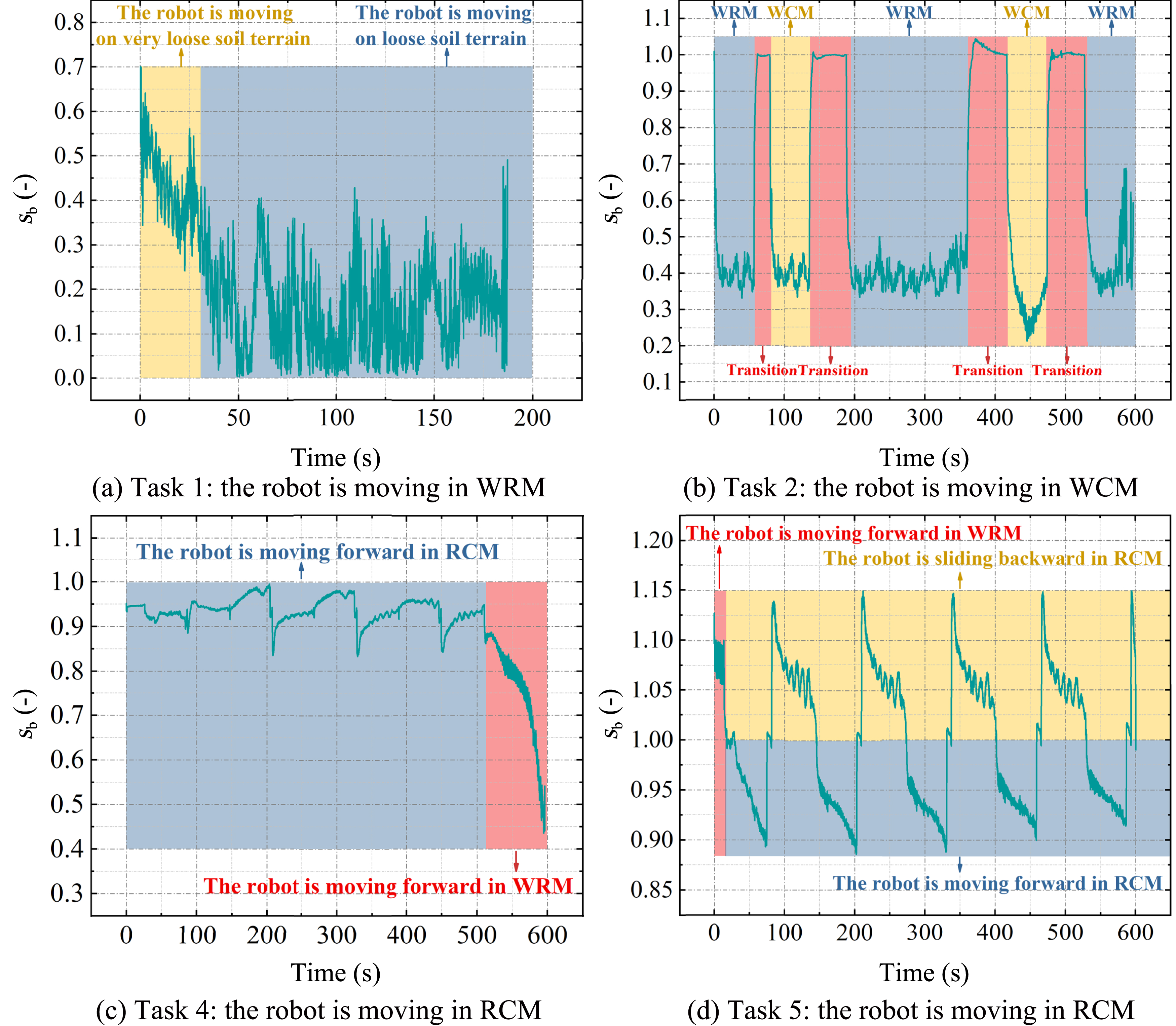

Above all, compared to the WRM, the defined WCM and RCLM are capable of efficiently avoiding obstacles at close range. The defined RCM is capable of escaping from robot sinking and climbing large slopes that the WRM cannot surmount. The defined SWLM and DWLM are capable of dealing with certain special obstacles located ahead of the wheels and climbing the upper surfaces of obstacles.

Remark 7

Different degrees of looseness can be set by the soil with the same terrain mechanical properties. For instance, freshly turned soil and compacted soil will present different wheel–terrain interaction states to the robot. In this study, the freshly turned sandy loam is defined as “very loose soil,” while the compacted soil is defined as “loose soil.”

8.5. Results of enhanced mobility achieved by the robot through multimode motion capabilities

The operational mobility of the robot on soil terrain with various obstacles was validated through multimode motion in experimental Tasks 1−7. To support the effective application of multimode control, the motion efficiency indices (s_b, traction efficiency PE, traction coefficient PC) and energy efficiency metrics (driving power P of the robot and its energy consumption E_C) were utilized to analyze the experimental results of Tasks 8−13. The analysis involved a comparison of maximum body traction, minimum slip ratio, and minimum obstacle traversal/avoidance time across six defined motion modes.

In Task 8, the robot was controlled to follow a straight-line path at three different velocities (5, 15, 25 mm/s), with time-series changes, while maintaining equal travel time (60 s) for each constant velocity. The used terrain consisted of loose soil that was approximately flat but featured an uneven distribution of sandy loam texture. As the traveling velocity v_b increased from 5 mm/s to 15 mm/s and then from 15 mm/s to 25 mm/s, the s_b value increased from 0.32 to 0.41 and from 0.02 to 0.31, respectively, as shown in Figure 17(a). The transition time for different velocity changes was approximately 4 s during experiments with v_b controlled at 15 mm/s and 25 mm/s. In these movements, the rapid increase in s_b was mainly due to the terrain rutting caused by the robot’s acceleration, during which the wheels momentarily moved both forward and downward at an angle, resulting in a small incline. This phenomenon was primarily caused by the heavy weight of the robot (225 kg), the structure of the wheel spur, the slow movement velocity, and the loose soil characteristics. Conversely, when v_b decreased from 25 mm/s to 15 mm/s and then from 15 mm/s to 5 mm/s, s_b decreased from 0.22 to 0.05 and from 0.25 to −0.25, respectively, with an observed forward sliding motion. In addition, s_b fluctuated within a range of 0.18 to 0.32 during constant-velocity motion across different velocities. As a result, when v_b is increased, the variation range of s_b is significantly enlarged, while when v_b is decreased, it is noticeably reduced. Once a constant v_b is maintained, the s_b values at various velocities are similar, varying within the range of 0.18 to 0.32. It is demonstrated that differences in the constant value v_b do not significantly affect s_b variation.

Figure 17.

Slip ratio, traction, driving power, energy consumption analysis of the robot with WRM in Task 8.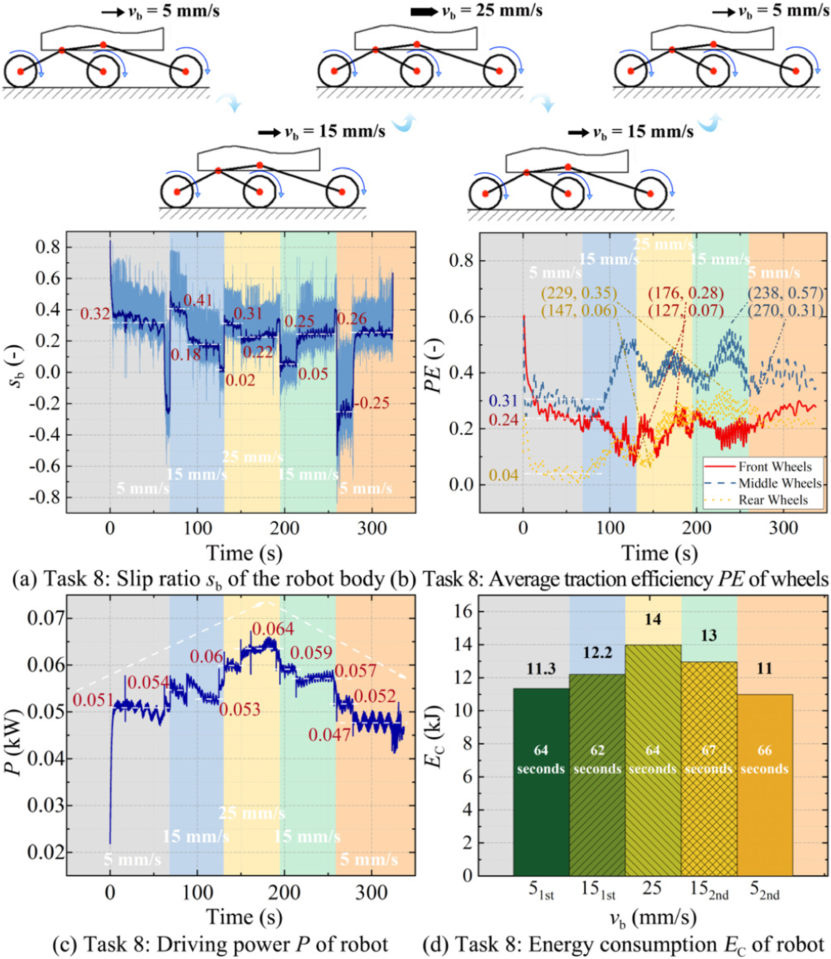

Furthermore, the PE in a robot was calculated using equation (43), and shown in Figure 17(b).

P E = \frac{1}{n} \sum_{m = 1}^{n} \frac{F_{DP, m} \cdot r_{s}}{T_{m}}

(43)

where F_DP,m denotes the drawbar pull on the m-th wheel, and T_m denotes the corresponding driving torque; in addition, n is determined by the expression n = 6 − c, and c is used to denote the number of lifted wheels.

Four motion tasks of the robot were drawn to verify the control system’s performance. During the velocity transition of 15-25-15 mm/s, the average PE of the middle and rear wheels was not significantly affected by velocity changes, remaining stable within ranges of 0.61–1.02 and 0.54−0.93, respectively. However, a monotonic increase in the average PE was shown by the front wheels. At the initial low-speed movement of 5 mm/s, the front wheel’s PE (0.62) was lower than that of the middle (0.92) and rear (0.78) wheels. As the v_b increased, the front wheels’ PE gradually increased, up to 1.02. Meanwhile, the PE of the middle and rear wheels stabilized in a certain range to support the forward motion. This trend in PE variations was mainly attributed to terrain features and the suspension structure: the front wheels traversed relatively flat loose surfaces while connected to a locked active-rocker arm, minimizing vertical velocity. In contrast, the middle and rear wheels encountered more compact soil terrain caused by ruts created by the front wheels. Compared to rear wheels, the forward traction transferred from the front and middle to the body is larger during relatively high-speed motion. Moreover, as v_b increased from 5 mm/s to 25 mm/s, the P value increased from 0.051 kW to 0.064 kW. In contrast, as v_b decreased from 25 mm/s to 5 mm/s, P decreased from 0.064 kW to 0.047 kW, closely matching the trends of v_b variations, as shown in Figure 17(c). The E_C at different velocities, depicted in Figure 17(d), showed values of 11.3 kJ, 12.2 kJ, 14 kJ, 13 kJ, and 11 kJ for velocities of the first 5, the first 15, 25, the second 15, and the second 5 mm/s, respectively. Higher E_C was observed during acceleration, while lower E_C occurred during deceleration, resulting in consistent trends between E_C and P.

To ensure effective mobility while minimizing the risk of sinking into the terrain across diverse environments, an adaptive velocity control strategy for WRM is concluded as follows: the fewer the v_b levels with incremental steps, the less the staged increase in s_b. During transitions or when higher motion efficiency is required on flat terrain, a moderate v_b value should be utilized, with close monitoring of the robot’s E_C and PE.

In Task 9, the improvement in steering performance achieved by the WCM was validated by comparing it to the WRM that uses the Ackermann steering model in an obstacle avoidance scenario, leading to the same end position. As shown in Figure 18(a), the s_b ranges for WRM (Ackermann) and WCM were (0.27, 0.5) and (0.13, 0.37), respectively. Their corresponding average s_b values were 0.41 and 0.31, indicating that a smaller variation was maintained by the WCM, resulting in a reduction in the risk of wheel sinking. Additionally, running times of 289 s and 271 s were recorded for WRM (Ackermann) and WCM, respectively, with the WCM reducing the time by 6.2%. As depicted in Figure 18(b), the PE of WRM (Ackermann) and WCM vary within 0.18–0.69 and 0.15–0.52, respectively, both showing a monotonically increasing trend. It is worth noting that the initial PE value of the WCM was negative, which was caused by the in-situ rotation of the wheel to a certain angle. During this period, the F_DP value was changed by the terrain deformation while the wheels remained stationary in the forward direction.

Figure 18.

Slip ratio, traction, driving power, energy consumption analysis of the robot with WCM in Task 9.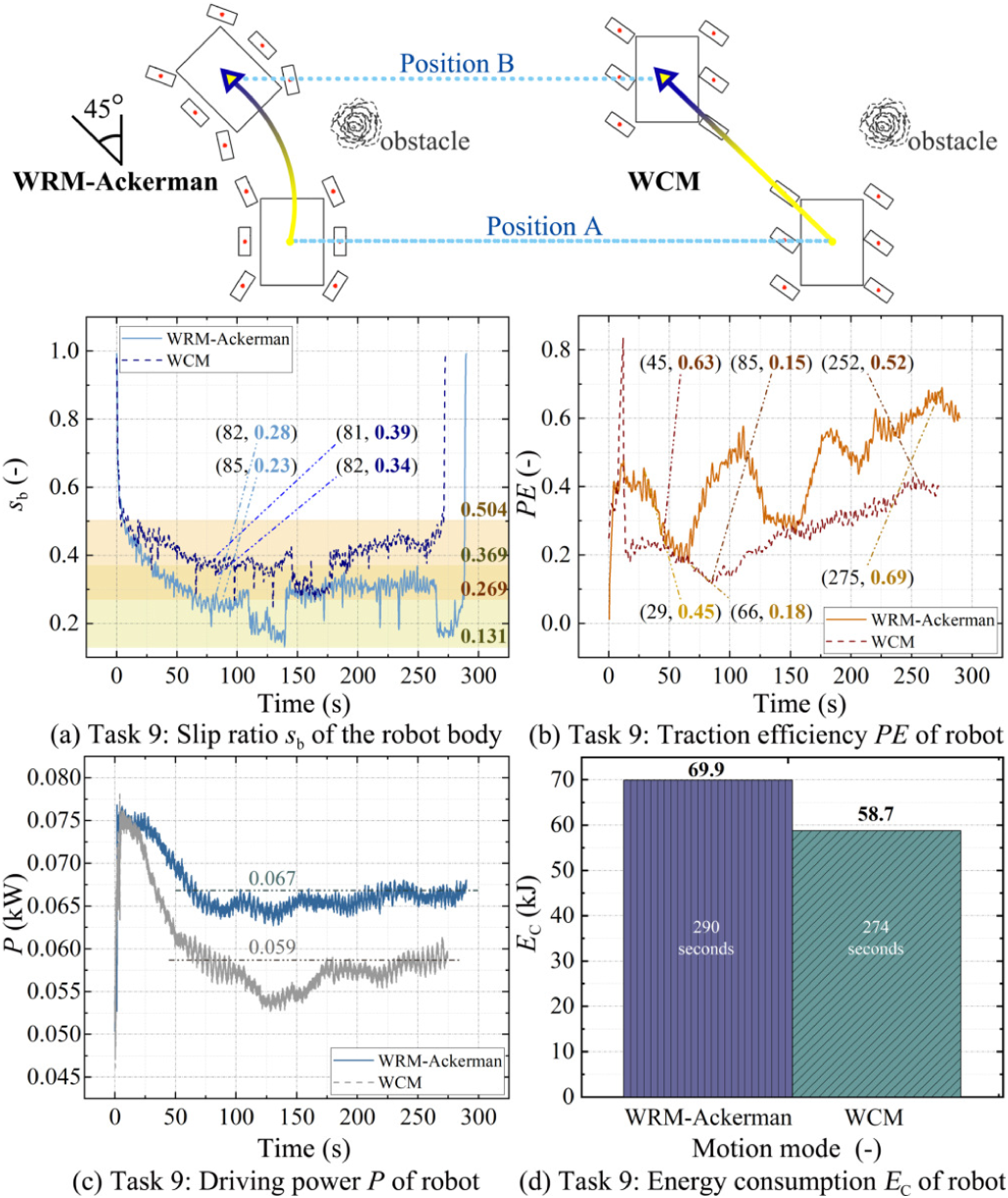

According to Figure 18(b), a larger amplitude of PE fluctuation was observed for the WCM during the initial phase of motion compared with the WRM (Ackermann). This was attributed to a small climbing process, where a 3.5 cm vertical height change of the body box occurred. In contrast, under similar terrain conditions, a 0.17 cm vertical height difference was experienced by the robot using the WRM (Ackermann).

As shown in Figure 18(c), the P of the robot when using the WCM (with an average value of 0.059 kW) was lower than that of the WRM (Ackermann) (with an average value of 0.067 kW). The variation trends of P were consistent with those of PE. In Figure 18(d), the E_C of 58.7 kJ was recorded by the WCM, representing a 15.9% reduction compared with the HIT-MRII robot employing the WRM (Ackermann) (69.9 kJ), while still avoiding the same obstacle and reaching the same target position.

To optimize motion control using WCM in a robot, through real-time wheel reorientation and coordinated steering control, the robot is capable of maintaining a lower risk of wheel sinking, improving motion time, and achieving more efficient power consumption. Consequently, incorporating the WCM into the path planning of the robot’s control system and its steering modules enables more robust obstacle avoidance, and fast curved locomotion compared to a conventional Ackermann-based configuration. In multi-obstacle scenarios, according to the variation in safe distance between the robot and obstacle, crucial advantages in maneuverability were demonstrated by the WCM, particularly when the steering curvature achievable by WRM (Ackermann) was insufficient.

In Task 10, the robot chassis height was sequentially changed by the RCLM at four different heights—250, 450, 150, and 550 mm—while a straight-line path on loose soil terrain was followed. To minimize the number of variables, the wheel velocity distribution was coordinated through the defined MC #2, ensuring that the commanded s_b (15 mm/s) remained constant throughout the experiment. During movements at chassis heights of 250 mm, 250–450 mm, 450 mm, 450–150 mm, 150–550 mm, and 550-250 mm, the value of v_b was observed to remain between 0 and 0.44, as shown in Figure 19(a).

Figure 19.

Slip ratio, traction, driving power, energy consumption analysis of the RCLM in Task 10.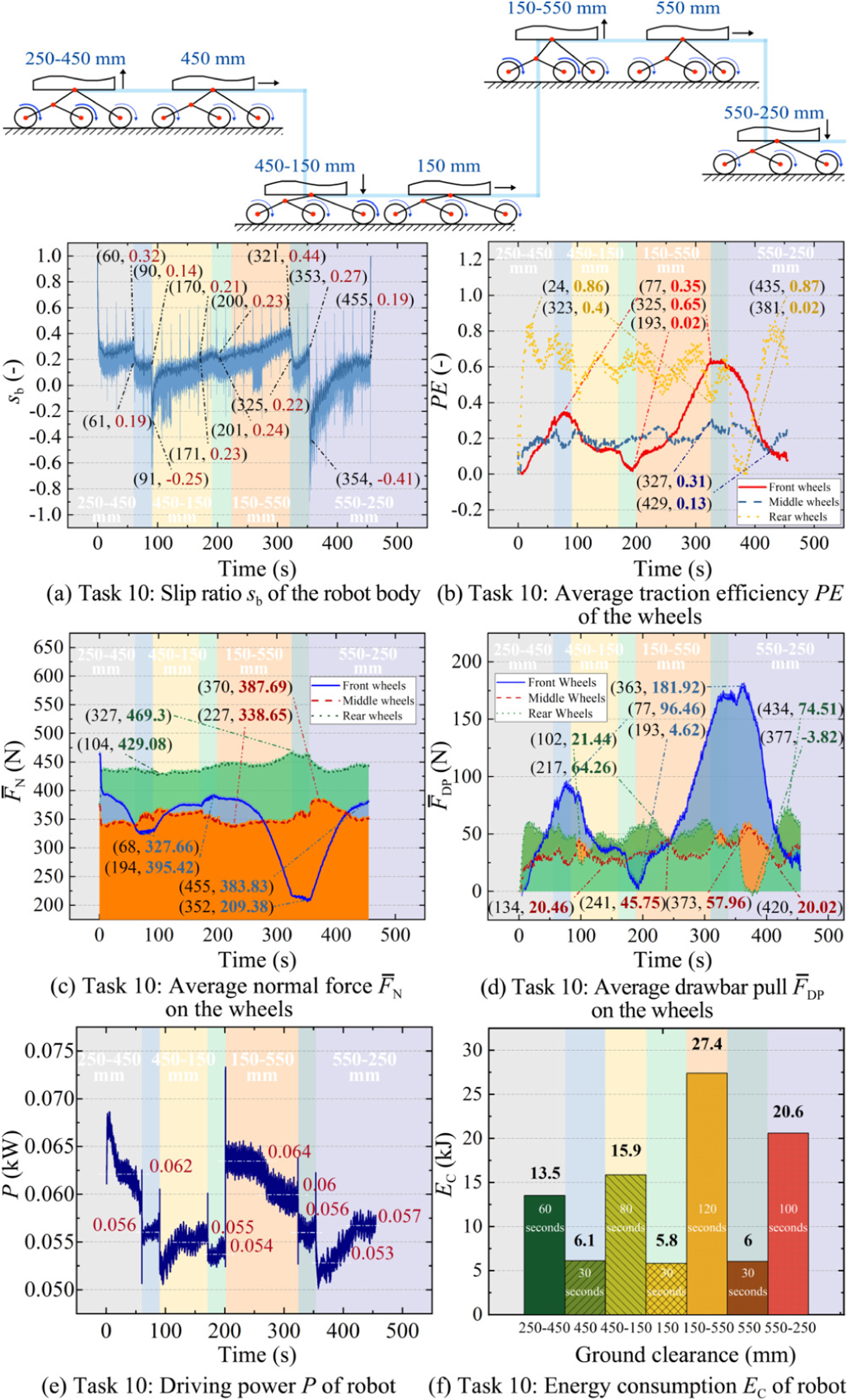

In the initial phase, when the chassis height was lowered from 450 mm to 150 mm, v_b increased abruptly, causing s_b to become negative. However, during the transition from 150 mm to 550 mm, s_b was observed to change smoothly. This difference was attributed to the distinct effects exerted by the movement of front and middle/rear wheels on the position of the robot’s CoM. Specifically, variations in the front-wheel velocity were transferred more directly to the CoM through the active suspension rockers, whereas part of the velocity variation from the middle/rear wheels was decreased by the passive suspension. In the final stage of chassis height adjustment (from 550 mm to 250 mm), the v_b changed rapidly due to the acceleration of the front wheels, causing s_b to vary suddenly. Furthermore, when the front wheels moved closer to the middle wheels (i.e., when the wheelbase was shortened), the v_b velocity first increased, and then maintained a similar proportional relation.

Remark 8

The v_b value was determined based on the movement of the CoM position, and was subsequently utilized in the calculation of s_b. In the coordination of wheel velocity settings, the chassis is raised by accelerating the middle and rear wheels, while it is lowered by accelerating the front wheels.

Moreover, the average PE of the middle wheels remained within a stable and narrow range—0.13 to 0.31—as illustrated in Figure 19(b). This finding indicates that the middle wheels’ PE were minimally influenced by changes in chassis height. In contrast, the average PE of the rear wheels varied significantly, ranging from 0.4 to 0.86 as the chassis height was increased from 250 mm to 550 mm. When the chassis height was subsequently decreased from 550 mm to 250 mm, the rear wheels’ PE dropped sharply to 0.02 before recovering to 0.87. This phenomenon was primarily caused by the counterclockwise rotation of the rear rocker in the active suspension while the chassis height was being lowered. The rear wheel, which was moving forward, experienced an intensified backward thrust force, leading to a sudden decrease in its F_DP and a consequent decrease in PE. As the robot continued moving, the posture shift in the passive suspension allowed the rear wheel to return to normal motion. Meanwhile, the average PE of the front wheels showed a two-phase trend. When the chassis height was adjusted from 250 mm to 450 mm, then to 150 mm, and finally to 550 mm, the PE remained stable (0.02 to 0.33). Upon reaching 550 mm, the PE peaked at 0.65. As the chassis was lowered from 550 mm back to 250 mm, the PE returned to its initial range.

These abrupt changes in the PE of the front and rear wheels were observed to coincide with significant variations in their F_N and F_DP. The average F_N of the front wheels was found to fluctuate initially between 327.66 N and 395.42 N, and subsequently between 209.38 N and 383.83 N, while the average F_DP varied between 4.62 N and 94.46 N and later between 20.10 N and 181.92 N. These results indicate that the degree of variation in F_DP is larger than that of F_N. As shown in Figures 19(c) and (d), the magnitude of these force variations was observed to increase significantly during the raising and lowering of the chassis, while more moderate changes occurred when the chassis height remained stable. In contrast, the average F_N of the rear wheels showed relatively stable changes, but significant fluctuations in the average F_DP were recorded across two phases, ranging from 21.44 N to 64.26 N and from −3.82 N to 74.51 N. The short occurrence of negative F_DP values was indicative of the forward sliding of the robot during these phases.

When the chassis height was maintained at a constant level, minimal differences in the P value were observed. For instance, at chassis heights of 150 mm, 450 mm, and 550 mm, P was measured at 0.054 kW, 0.056 kW, and 0.057 kW, respectively (Figure 19(e)). In terms of overall variation, P was found to decrease as the chassis height was raised and to increase as the chassis height was lowered. Additionally, a two-phase variation pattern in P was observed during each height adjustment: an approximately linear change with time in the first phase, followed by nearly constant values in the second phase. These observations indicate that the robot’s dynamic mechanical properties are segmented during suspension movement.

Regarding E_C, values of 5.8 kJ, 6.1 kJ, and 6.0 kJ were recorded when the chassis height was maintained at 150 mm, 450 mm, and 550 mm, respectively (Figure 19(f)). Upon raising the chassis by 200 mm, E_C rose to 13.5 kJ, averaging 6.8 kJ per 100 mm. For a 400 mm lifting height, E_C increased further to 27.5 kJ, corresponding to an average of 6.9 kJ per 100 mm. In contrast, when the chassis height was lowered by 300 mm, E_C was recorded at 15.9 kJ and 20.6 kJ, averaging 5.3 kJ per 100 mm and 6.9 kJ per 100 mm, respectively. Although the E_C for the two upward adjustments was nearly identical, a larger difference was observed for the two downward adjustments. It was noted that higher initial chassis heights led to less stability in the robot’s subsequent joint motions. As a result, to enhance the motion stability of the robot posture, in the cases where the chassis was lowered from high altitudes, the control parameters should be adaptively optimized based on the wheel–terrain interaction state.

To optimize motion control in a robot, the RCLM is capable of effectively maintaining optimal PE by automatically adjusting the distribution of wheels’ velocity and torque in real-time, accompanied by corresponding variations in chassis height. In order to keep a consistent v_b—particularly on uneven or loose terrains—while also improving E_C, the coordination of chassis height and suspension settings can be achieved by the RCLM utilization. This coordination ensures that the variations in F_N and F_DP remain stable within a certain range, which also contributes to the reduction of s_b.

In Task 11, the robot was controlled in two motion modes, RCM and WRM, to transition from flat, loose soil terrain to a 15° slope. During the RCM trial, the robot was initially driven in WRM mode on the flat terrain until the front wheels moved onto the slope. Meanwhile, the value of s_b was observed to rapidly increase to 0.98, as shown in Figure 20(a). At that point, the RCM mode was activated to keep moving forward, and then stabilize s_b with fluctuations around 0.44. By 3030 s, all wheels had successfully reached the slope. In the WRM trial, s_b linearly increased from the start of the movement, reaching 0.8. After the front wheels moved onto the slope surface, s_b decreased to 0.72. As the middle wheels arrived at the bottom of the slope, s_b continued to rise, eventually reaching 0.96. Subsequently, the health management protection system was triggered, causing the robot to halt. At this time, the robot had been running for 64 s, yet the middle wheels had not fully ascended the slope. These findings indicate that, compared to RCM, the WRM was unable to provide sufficient traction to facilitate an effective transition from flat terrain onto a loose soil slope.

Figure 20.

Slip ratio, traction, driving power, energy consumption analysis of the robot with RCM in Task 11.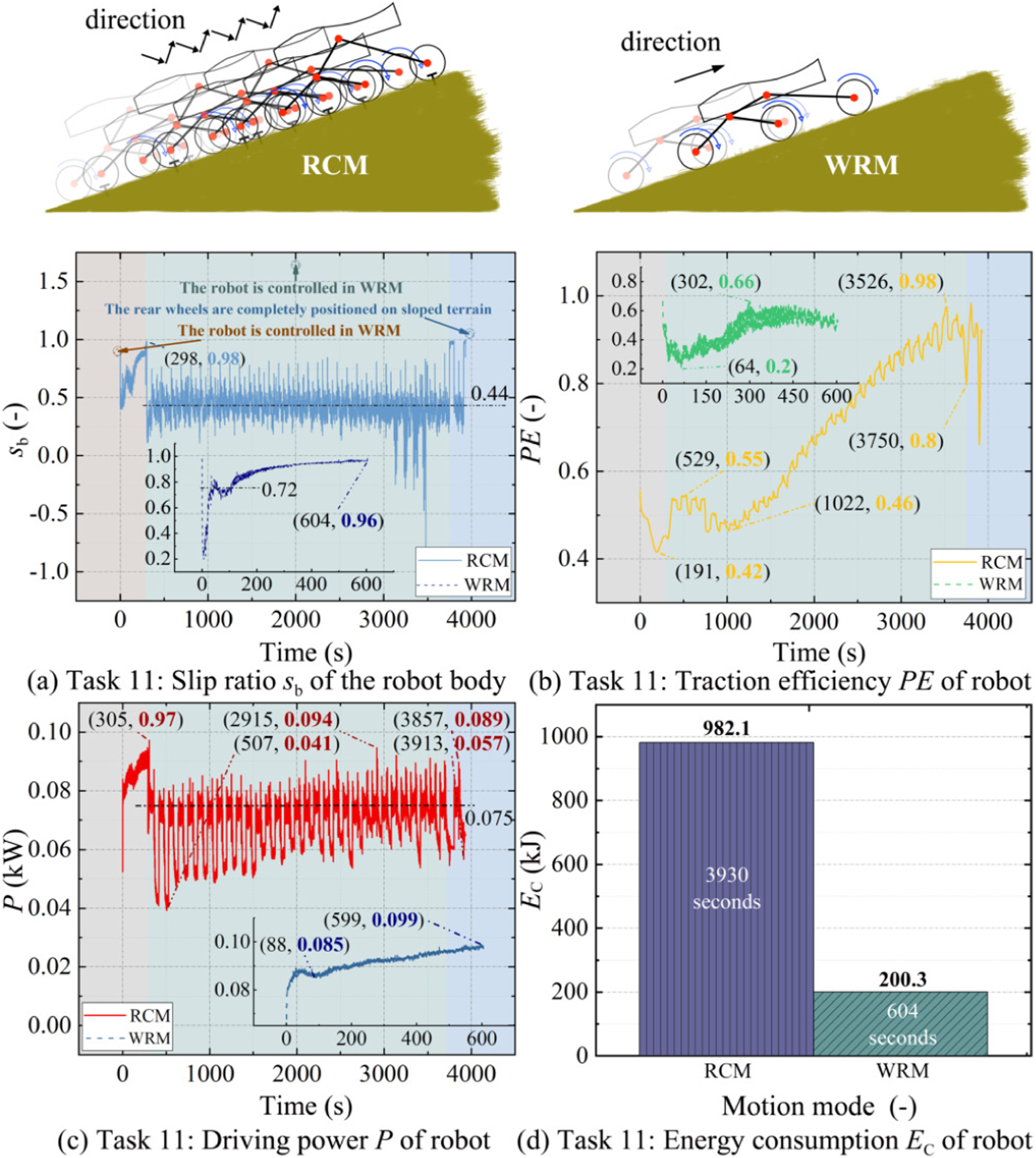

Remark 9

Although the WRM was utilized in both trials, differences in the observed s_b were attributed to the similar yet distinct terrain configurations. The soil loam texture was not set identically in the conducted experiments.

To PE variation, when the robot was controlled under RCM, the initial WRM movement caused a monotonic decrease, dropping to 0.42, as shown in Figure 20(b). Taking into account the avoidance of further declines, the motion mode was switched to RCM, after which PE rose to 0.55. As the middle wheels fully entered the slope, PE shortly dropped to 0.46 but then recovered to 0.98. Once the rear wheels were positioned on the slope, the PE value stabilized, showing only slight fluctuations with no significant drops. Under WRM control, the main trend of PE variation mirrored that of s_b; however, as s_b continued to increase, PE showed a downward trend. This result was consistent with the single-wheel test results Ding et al. (2011). Moreover, the P showed similar trends to s_b, as shown in Figure 20(c). In the RCM trial, P fluctuated between 0.041 kW and 0.094 kW. In the WRM trial, P monotonically increased, eventually reaching 0.099 kW. Regarding E_C, a total of 982.1 kJ was expended in the RCM trial, corresponding to an average of 0.25 kJ/s, whereas 200.3 kJ was consumed in the WRM trial, with an average of 0.33 kJ/s, as shown in Figure 20(d). Compared to WRM, RCM not only achieved the movement objective by allowing the robot to ascend the slope but also reduced average energy consumption by approximately 24.7%.

Remark 10

In the RCM calculation of E_C, the initial movement phase of the WRM was included, which implies that the actual energy efficiency improvement achieved by a single RCM exceeds the shown value of 24.7%.

To optimize motion control with the RCM in a robot, PE needs to be adjusted in real-time, preventing severe s_b and P spikes that frequently arise under WRM. In addition, the RCM should be activated as soon as undesirable trends in s_b and E_C are detected in certain movements, enabling the robot to traverse slopes more efficiently and reliably.

In Task 12, the robot’s mobility at various lifted heights from the ground with SWLM and DWLM was validated through a series of experimental trials. First, the front-right wheel was lifted to heights of 100 mm, 150 mm, and 200 mm on a loose soil surface covered with wooden planks, then moved forward for 900 mm at a v_b of 25 mm/s, and finally lowered to the ground. Next, both front wheels were raised to the same heights, moved forward over the same distance, and subsequently lowered to the ground. The experimental results are depicted in Figure 21, where triangular symbols denote sequential time markers. These symbols divide the suspension-wheel action stages during the lifting process, in accordance with Tasks 6 and 7.

Figure 21.

Slip ratio, traction, driving power, energy consumption analysis of SWLM and DWLM with different lifting heights of wheels in Task 12.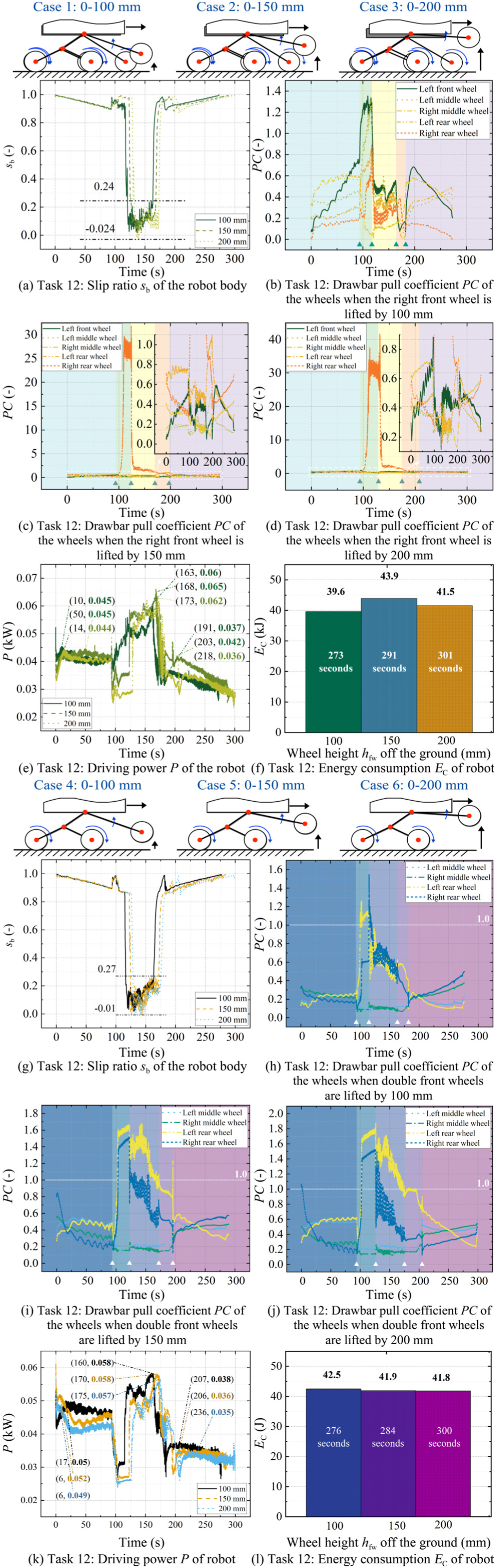

In the trials where the single front-right wheel was lifted, the s_b remained within 0.01–0.24, and did not show a marked overall change. A slight negative slip (s_b = −0.024) was observed when the wheel was lifted to 200 mm, as illustrated in Figure 21(a). To evaluate the traction performance per wheel load of the wheels, the PC is calculated by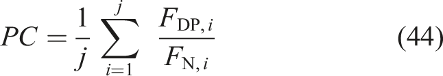

P C = \frac{1}{j} \sum_{i = 1}^{j} \frac{F_{DP, i}}{F_{N, i}}

(44)

where F_N,i indicates the normal force exerted on the i-th wheel, and j represents the total number of remaining wheels, excluding the lifted wheels.

Accordingly, these trials highlight the following findings:

• At 100 mm lifting height, the left front and left middle wheels showed PC values exceeding 1, indicating a disproportionate increase of F_DP than that of F_N (i.e., F_DP > F_N), as shown in Figure 21(b). The initial F_DP and F_N values before the lifting motion about 250 N and 380 N, respectively. The PC value of the other wheels followed the order: right middle wheel $>$ left rear wheel $>$ right rear wheel;

• At 150 mm lifting height, the F_DP and F_N on the lifted wheel are shown in Figure 22(a). The PC value of the right rear wheel exceeded 1, reaching 27.5, as shown in Figure 21(c). This excessive rise was due to a drop in F_N to 10 N, such that F_DP ≫ F_N. At this moment, the right rear wheel approached a suspended state, during which F_N was slightly increased from 10 N to 150 N in forward motion but remained below its nominal value of about 400 N. The F_DP was averaged around 210 N during the forward motion, as shown in Figure 22(b), of which the value is close to the initial. For other wheels, PC ranked as left rear wheel $>$ left front wheel $>$ right middle wheel $>$ left middle wheel;

• At 200 mm lifting height, the PC value of both rear wheels reached 32.5, as shown in Figure 21(d), and their F_N decreased to 8 N at the same time. With an increase in the height of the front-right wheel lift, a gradual rise in the maximum anomaly value of the rear wheel’s PE is observed, indicating a continuous intensification in the degree of hanging-on for the rear wheel. The PC sequence for the other wheels matched that at 150 mm lifting height.

Figure 22.

Drawbar pull and normal force of right front and rear wheels in SWLM in Task 12.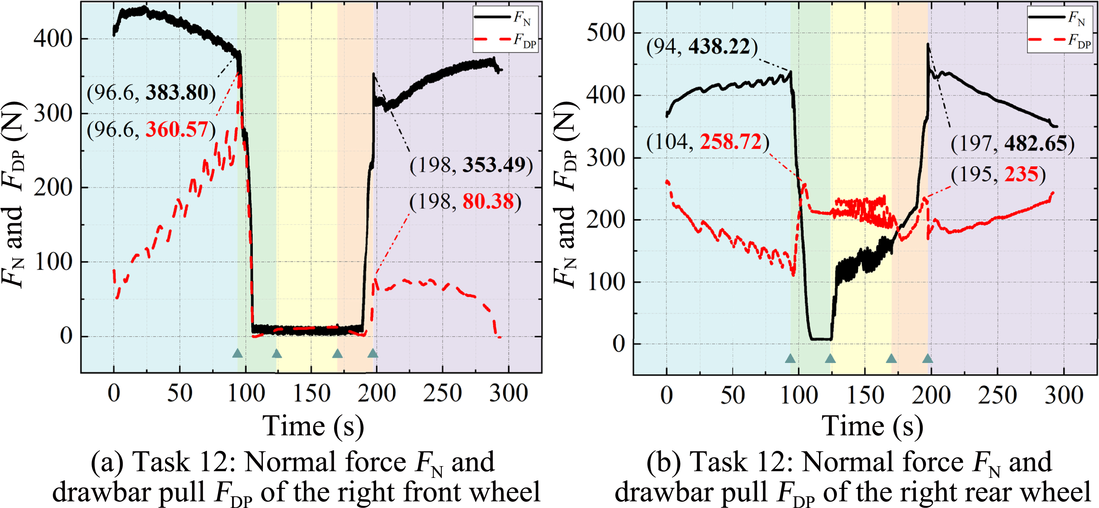

Regarding P variation, an average rise of approximately 0.03 kW was recorded as the lifting height increased from 100 mm to 150 mm, as shown in Figure 21(e). However, no further increase in P was noted at 200 mm, where the trend fell between the 100 mm and 150 mm results. Specifically, the E_C values were 39.6 kJ, 43.9 kJ, and 41.5 kJ, with average consumption rates of 6.9 kJ/s, 6.6 kJ/s, and 7.3 kJ/s, respectively, as indicated in Figure 21(f). These results demonstrate that the relation between P and lifting height does not follow a linear pattern, likely due to shifts in the body’s CoM and the resulting redistribution of wheel–terrain contact forces.

When both front wheels were lifted, the s_b ranged from −0.01 to 0.27 as the lifting height increased, as demonstrated in Figure 21(g). The recorded negative values of s_b were found to induce fluctuations in v_b and relative chassis slip, which were mainly caused by motion inertia on the loose soil terrain. Furthermore, the analysis of PC variation provides the following insights:

• At 100 mm lifting height, the PC of both middle wheels was considerably lower during the wheel lifting phrase, at around 0.1, as shown in Figure 21(h). In contrast, PC values for the rear wheels were initially observed to exceed 1, aligning with the findings of the SWLM, and subsequently stabilized around 0.6.

• At 150 mm and 200 mm lifting heights, the PC values appeared almost identical at both heights, indicating a small effect of increased lifting height on PC. The PC of the middle and rear wheels followed patterns similar to those at 100 mm, though with slightly larger values, as shown in Figures 21(i) and (j).

In terms of P value, a downward trend was generally noted as lifting height increased, contrary to the outcome from SWLM. The average difference of P was measured to be approximately 0.004 kW between the 100 mm test and the 150 mm test, while a difference of less than 0.002 kW was observed between the 150 mm test and the 200 mm test, as presented in Figure 21(k). In addition, the E_C values were 42.5 kJ, 41.9 kJ, and 41.8 kJ, corresponding to consumption rates of 0.154 kJ/s, 0.148 kJ/s, and 0.139 kJ/s, respectively, as shown in Figure 21(l). In comparison with the SWLM trial, the DWLM trial led to a slight decrease in average E_C with increasing height, demonstrating the nonlinear relation between lifting height, P, and E_C.

A comprehensive single-wheel lifting control experiment was performed for various heights. The lifting height should be constrained within a range suitable for terrain adaptations. Significant shifts in the body’s CoM position will be generated by excessive wheel lifts, resulting in a pronounced nonlinear variation in the distribution of wheel–terrain contact forces. To stabilize s_b and achieve optimal E_C, real-time monitoring of F_DP and F_N variations is essential for dynamically adjusting P. Effective coordination of wheel load distribution and drive control is required to balance PC and E_C during wheel lifting operations.

In Task 13, to evaluate the impact of lifting wheels in different positions on the robot’s mobility, experiments were conducted in which either a single wheel or the front, middle, and rear pairs of wheels were lifted to a height of 200 mm. The robot was subsequently directed to travel 900 mm along a straight path before the wheels were returned to the ground. The same experimental setup as in Task 12 was employed.

When a single front, middle, or rear wheel was lifted, minimal changes in s_b were observed, with values of (−0.1, 0.14), (−0.16, 0.1), and (−0.02, 0.21), respectively, as shown in Figure 23(a). Short instances of forward slippage were recorded, with the most significant slippage occurring when the right rear wheel was lifted, and the least when the right front wheel was lifted. This outcome indicates that the rear wheels exert the largest influence on the robot’s CoM position, while the front wheels exert the least.

Figure 23.

Slip ratio, traction, driving power, energy consumption analysis of SWLM and DWLM with different position distribution of wheels in Task 13.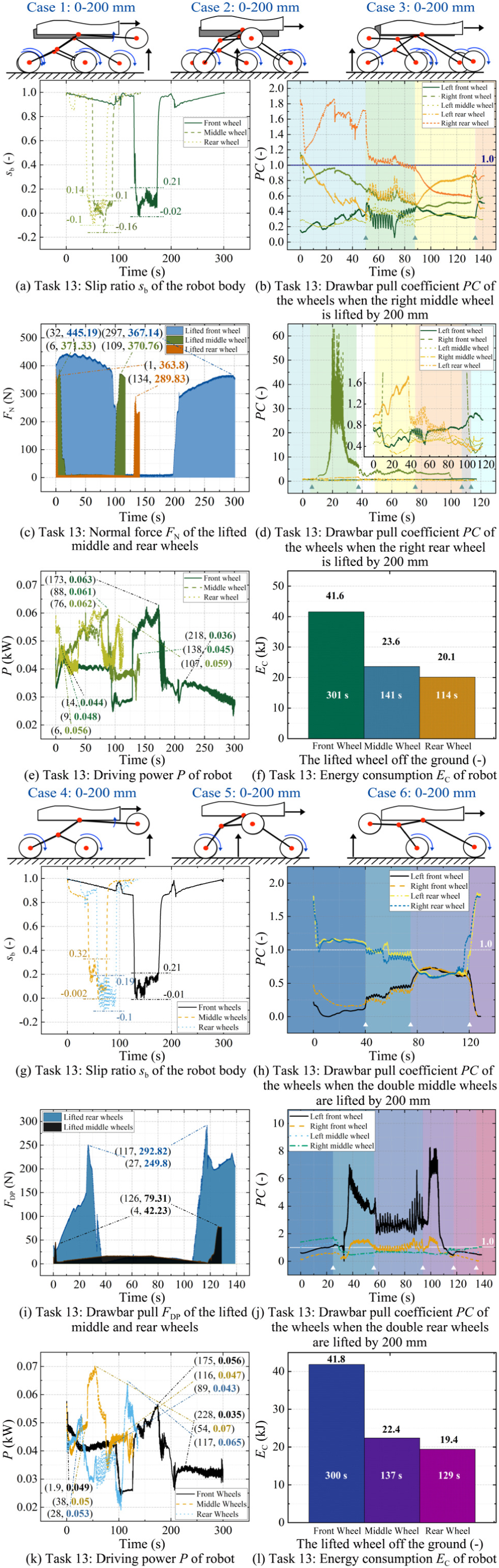

In terms of PC, lifting the right middle wheel caused PC to exceed 1 for the right rear wheel. Meanwhile, the PC values for the right front and left rear wheels were approximately 0.6, and those for the left front and middle wheels were about 0.3, as illustrated in Figure 23(b). In this case, approximately 370 N of F_N on the lifted right middle wheel was required to be redistributed and borne by the remaining wheels, as shown in Figure 23(c). When the right rear wheel was lifted, the PC of the left front wheel showed the largest variation, with an average of 35 and a peak exceeding 60, as shown in Figure 23(d). This large value can be explained by the “seesaw principle,” since the left front wheel opposed the lifted right rear wheel, and experienced a significant decrease in F_N. The left rear wheel reached a PC of 1.6, whereas the PC values of the other wheels remained between 0.4 and 0.7, redistributing approximately F_N = 300 N from the lifted right rear to the remaining wheels, as depicted in Figure 23(c). Moreover, during forward motion, the P peak for single-wheel lifting was similar across the front, middle, and rear wheels, at approximately 0.063, 0.061, and 0.062 kW, respectively, as shown in Figure 23(e). Total E_C was 41.6 kJ, 23.6 kJ, and 20.1 kJ for lifting front, middle, and rear wheels, respectively, as depicted in Figure 23(f), and the corresponding consumption rates are 0.138 kJ/s, 0.167 kJ/s, and 0.176 kJ/s. Although the lowest E_C per unit time was achieved by lifting the single front wheel, its total E_C was nearly double that of the middle and rear wheels.

For DWLM trials, the s_b trends were consistent with those from single-wheel lifting, as shown in Figure 23(g). Lifting the middle wheels resulted in an s_b peak of 0.32, over three times that of a single middle wheel, while forward sliding was negligible. Compared to single rear-wheel lifting, the frequency of the body’s forward sliding is increased in the case of lifting the rear wheels, with a peak of −0.1. Negligible slippage was observed in the trial of lifting the front wheels, as indicated by an s_b range of (−0.01, 0.21), which is comparable to the range observed for a single front wheel. As illustrated in Figure 23(h), the rear wheels were caused to exceed a PC value of 1 due to the double middle-wheel lifting, while remaining below 1.25. Simultaneously, the front wheel’s PC was incrementally increased from 0.2 to 0.7, redistributing approximately 60 N of F_DP from the lifted wheel onto the remaining wheels, as shown in Figure 23(i). The PC of the middle wheels was caused to exceed 1 during the double rear-wheel lifting but dropped below 1 afterward, as shown in Figure 23(j). During forward motion, the left front wheel exhibited substantial PC variations, peaking at 8 with an average surpassing 3, while the right front wheel’s PC exceeded 1. Meanwhile, approximately 270 N of F_DP was redistributed to the wheels on the ground, as shown in Figure 23(i). Large differences in PC were induced by simultaneous lifting of the two front wheels, which was likely caused by uneven terrain, as asymmetric tilting of the sand–soil base was observed.

The P value during double front- and middle-wheel lifting remained similar to that of corresponding single-wheel lifting, as shown in Figure 23(k). However, compared to the trial of single rear-wheel lifting, double rear-wheel lifting led to an approximately 50% reduction in P. The E_C values for double front-, middle-, and rear-wheel lifting were 41.8 kJ, 22.4 kJ, and 19.4 kJ, respectively, as shown in Figure 23(l). These values correspond to an increase of 0.6%, a decrease of 5.4%, and a decrease of 3.4% compared to single-wheel lifting, demonstrating that DWLM does not necessarily consume more energy than SWLM.

In motion control of a robot, both SWLM and DWLM can be utilized to traverse obstacles, and optimize wheel–terrain interaction as well as E_C in rough-terrain driving. SWLM is particularly suited for fine-tuning load distribution when minor s_b compensation or moderate PC adjustments are required. DWLM can be applied to achieve more substantial wheel load redistribution without necessarily increasing total E_C. Rear-wheel lifting results in the most significant impact on the robot’s CoM. Consequently, SWLM or DWLM (front, middle, or rear) should be chosen based on the specific task objectives among slip mitigation, traction redistribution, and energy efficiency. The enhanced mobility and key findings from the above six experiments of multimode traversal comparisons are listed in Table 5.

Table 5.

Overview of HIT-MRII multimode traversal across soil terrain and wooden ground, summarizing key application strategies and control insights in Tasks 8–13.

Task	Motion mode	Key application strategy	Control insights
Task 8	WRM	Lower frequency of v_b step-over increase is conducive to decrease s_b, and consequently enhance motion safety. Larger v_b is recommended for higher movement efficiency on flat terrain, with E_C and PE monitored	Minimized risk in terrain sinking by adaptive velocity control of WRM while ensuring high traction efficiency across diverse flat terrains
Task 9	WCM	Real-time wheel reorientation and steering can be utilized to lower the risk of sinking, reduce motion time, and improve power efficiency	WCM can be integrated into trajectory planning and steering modules. Robust obstacle avoidance and reduced running time in multi-obstacle scenarios
Task 10	RCLM	Velocity and torque of the wheels and suspension rockers are coordinately adjusted in real-time to maintain a large PE. Chassis height can be dynamically changed to stabilize the F_N and F_DP of the wheels within a controlled range	A consistent robot’s traveling velocity for efficient traversal on uneven terrains can be ensured by the RCLM, which enhances energy efficiency and reduces body slip
Task 11	RCM	PE can be adjusted by changing wheelbase length at a certain frequency to mitigate undesirable trends in s_b variations and P spikes, leading to the prevention of a surge in E_C	Efficient and reliable slope traversal can be achieved through the RCM, which overcomes the limitations of the WRM in traction-deficient conditions
Task 12	SWLM & DWLM with varying wheel lifting heights	Lifting height can be confined within terrain-adaptive ranges to prevent shifts in the body’s CoM and inefficiencies. The forces F_DP and F_N on the wheels can be dynamically adjusted by varying the lifting heights to stabilize s_b and optimize E_C	In SWLM and DWLM, balanced traction and energy efficiency can be achieved through effective wheel load distribution, which is managed by adjusting the lifting heights of the wheels
Task 13	SWLM & DWLM with various lifted-wheel positions	Significant variations in the position of the body’s CoM are influenced by the lifting height of rear wheels, while considerable increases in E_C result from the lifting height of front wheels	SWLM can be used for fine load distribution and moderate PC adjustments, while DWLM can be utilized for substantial load redistribution without increasing total E_C

Note 3

In experimental Tasks 8–13, to simplify the description, the motion control parameters not explicitly mentioned were configured identically to those specified for the corresponding motion modes in Tasks 1–7.

To support the multimode mobility summary in Table 5 with a comparative evaluation, Task 14 was designed as a representative obstacle-traversal scenario on loose soil. According to the movability limit of WRM, a medium-sized obstacle (150 × 550 × 190 mm), defined as not directly traversable in WRM, was placed on the nominal straight-line path. Under identical start/end conditions and a fixed commanded body speed (v_b = 15 mm/s), WRM (Ackermann), WCM, RCLM, and SWLM were executed and evaluated in terms of travel distance, elapsed time, and energy consumption. The obstacle scenario and motion paths are shown in Figure 24, and the corresponding performance metrics are summarized in Table 6. For reference, the HIT-MRII dimensions are 2200 mm (length), 1700 mm (width), and an initial wheelbase of 1900 mm.

Figure 24.

Obstacle scenario and motion paths of WRM (Ackermann), WCM, RCLM, and SWLM in Task 14.

Table 6.

Comparison results of WRM (Ackermann), WCM, RCLM, and SWLM using travel distance, running time, and energy consumption in Task 14.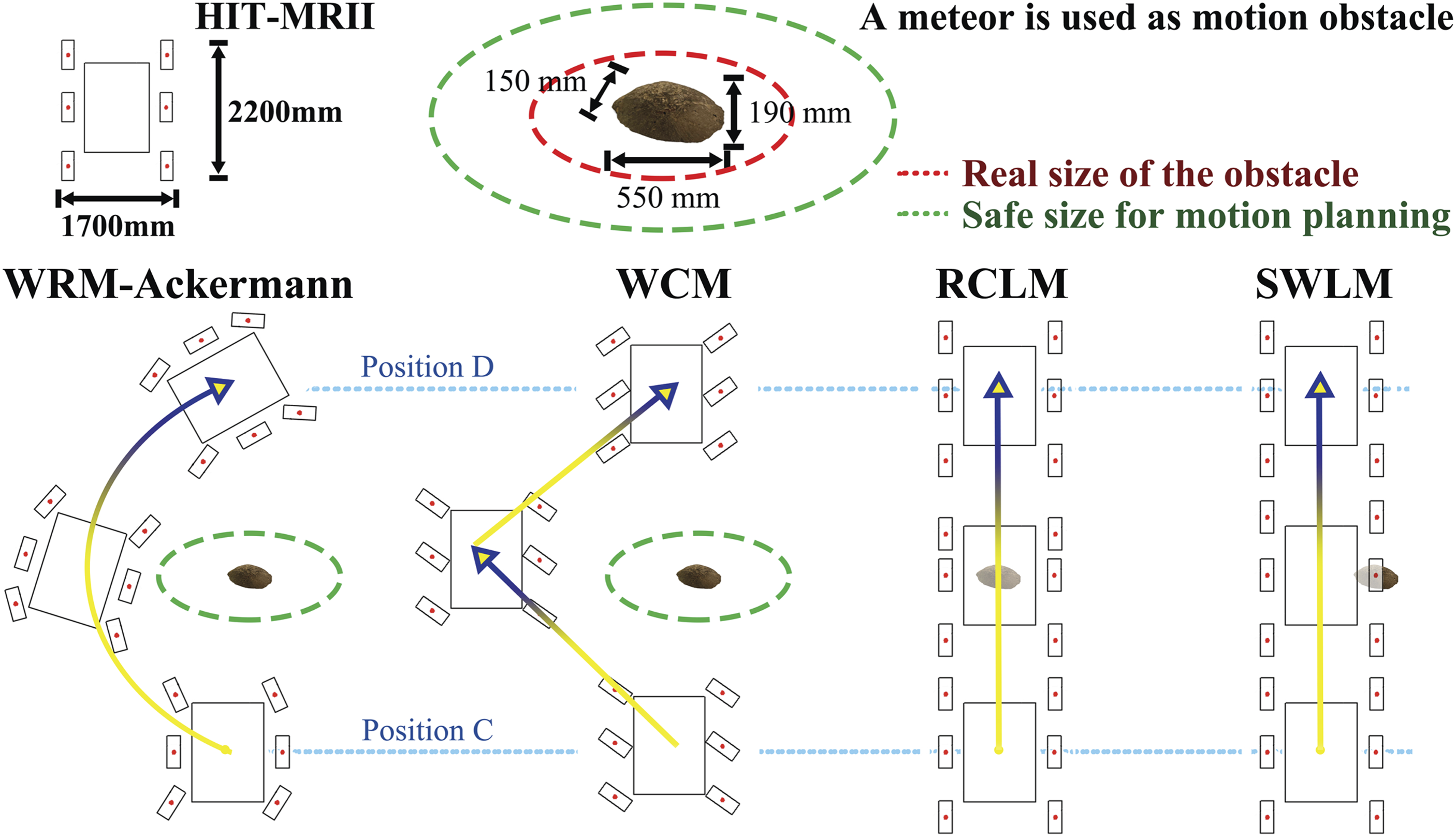

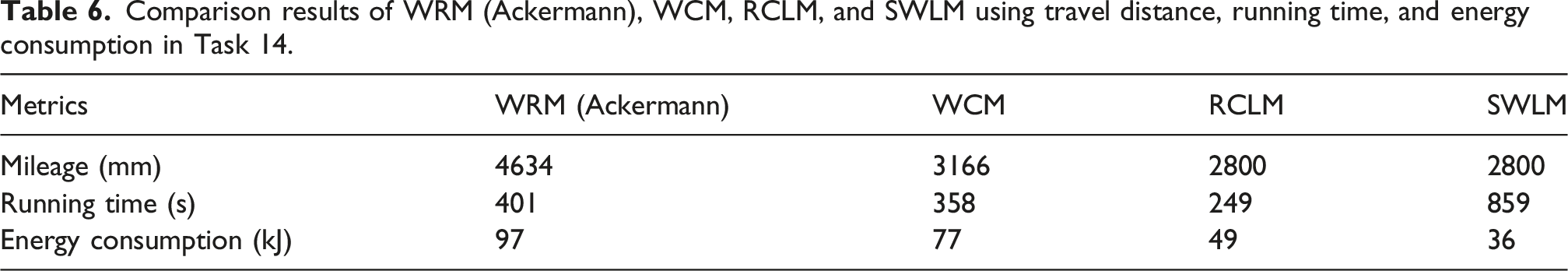
Metrics	WRM (Ackermann)	WCM	RCLM	SWLM
Mileage (mm)	4634	3166	2800	2800
Running time (s)	401	358	249	859
Energy consumption (kJ)	97	77	49	36

For obstacle avoidance, the starting point is set to the outer edge of the robot’s front wheels facing the obstacle at a distance of 300 mm, and the endpoint is set to the outer edge of the robot’s rear wheels facing the obstacle, also at a distance of 300 mm. Moreover, in the design of trajectory planning, a safe distance must be maintained along the avoidance trajectory using the WRM (Ackermann) and WCM. To ensure that a 300 mm safety margin is preserved while the obstacle is navigated around, the obstacle’s dimensions are expanded to calculate the trajectory of the robot’s central path. The expanded obstacle dimensions are 750 mm in the length direction (150 mm + 2 × 300 mm) and 1150 mm in the width direction (550 mm + 2 × 300 mm). In consequence, the size of the “expanded obstacle” that is circumvented by the robot’s center is 750 mm by 1150 mm. The command v_b is set to 15 mm/s in these trials.

According to the experimental results in Table 6, the WRM (Ackermann) moved the highest mileage, covering a distance of 4634 mm, which significantly exceeded the distances recorded by other modes. It indicates that longer travel paths can be achieved with the WRM when navigating around obstacles. The WCM was found to have the second-highest mileage at 3166 mm, while both the RCLM and SWLM recorded the shortest distances, each at 2800 mm. In terms of running time, the SWLM was noted as the slowest, taking 859 s to complete the task. By contrast, the RCLM was observed to be the fastest, completing the task in just 249 s, followed by the WCM and WRM (Ackermann) at 358 s and 401 s, respectively. E_C data revealed that the SWLM was the most energy-efficient, consuming a minimum of 36 kJ, followed by the RCLM at 49 kJ and the WCM at 77 kJ. The WRM (Ackermann) showed the highest E_C, recorded at 97 kJ.

The differences observed in the experimental results demonstrate that each mode possesses specific advantages and is suited for distinct obstacle-related applications on soil terrain conditions. The WRM (Ackermann) is particularly effective when obstacles need to be avoided over longer travel distances, as smooth and continuous path tracking is ensured. However, its higher energy consumption and relatively longer running time should be taken into account in such applications. Similarly, the WCM mode is well-suited for avoiding obstacles while achieving a balance between mileage and energy efficiency, as it can maneuver effectively around obstacles in short-distance scenarios. In comparison to the WRM (Ackermann), the WCM is considered more suitable for use in environments where energy efficiency is regarded as a critical factor.

Conversely, the RCLM is optimized for the direct traversal of obstacles, especially in tasks requiring rapid completion and low energy consumption. This mode is particularly advantageous for ensuring the optimal stability of the robot’s body posture during obstacle crossing. However, its effectiveness is dependent on the precise alignment of the obstacle relative to the robot’s chassis, which restricts its flexibility in some situations. In contrast, the SWLM mode provides optimal flexibility during obstacle traversal due to its reduced reliance on precise obstacle positioning relative to the robot. It is particularly effective for navigating narrow terrain and unavoidable obstacles that require adaptive movement, with superior energy efficiency.

8.6. Results of the improved differential steering

The control performance of the built differential steering model was verified in Task 15 using the HIT-MRII robot. During the steering motion with two desired angular velocities ω_b of the body at 0.02 rad/s and 0.03 rad/s, the wheelbase length was increased by lowering the robot chassis. In consequence, the steering angular velocity is decreased with the increase of the wheelbase length. As shown in Figure 25(a), the angular velocity maintains mainly a stable changing trend of decreasing. On the other hand, the steering angle maintained a stable increase, while the value of corresponding angular velocity had short, and rapid fluctuation, as shown in Figure 25(b). Consequently, in the case of an increase in the wheelbase length during the robot’s motion, the results demonstrate efficient control performance to ensure stable steering in the horizontal plane. In addition, the initial ω_b of one trial is set to 0.02 rad/s, and the average ${\bar{ω}}_{b}$ is 0.003 rad/s, resulting in the robot motion with increasing wheelbase length. The robot’s motion remains consistently aligned with the desired performance on loose sandy terrain, using the developed 3D kinematic model.

Figure 25.

Task 15: Steering angle, angular velocity, and motion constraints of the robot with the built 3D differential-drive model.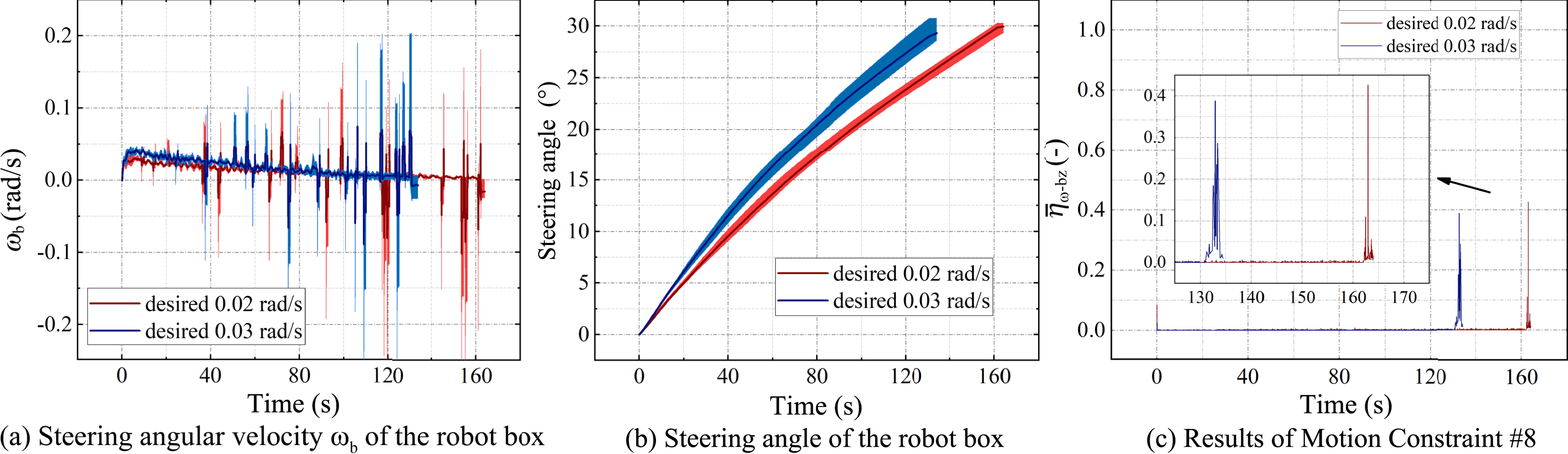

Moreover, the task involves MCs #6 and #8. A more substantial change in steering angular velocity is observed during the final phase of steering movements compared to other steering processes. However, the time and the changing frequency of the fluctuations are short and small, respectively, as shown in Figure 25(c). Accordingly, for MC #6, the control parameters of the differential model are similar to those of the lowering part of the RCLM in Task 3. The maximum values η_ω−bz for MC #8 at ω_b = 0.02 rad/s and ω_b = 0.03 rad/s are around 0.4, which are below the preset threshold of ${\bar{η}}_{ω - b z} = 0.7$ .

In the in-situ steering experiment on loose soil, the HIT-MRII robot was commanded to rotate about its vertical axis with constant desired body yaw rates ω_b,d = 0.01 rad/s and 0.02 rad/s. Over t ∈ [0, T_s], the yaw angle ψ(t) and its rate ${(ω_{b})}_{z} (t)$ were recorded, and the tracking error was defined as $e_{ω} (t) = {(ω_{b})}_{z} (t) - ω_{b, d}$ . Two trials were conducted with T_s = 282 s and 146 s, and Δψ = ψ(T_s) − ψ(0) was 0.61 rad in both trials. The mean achieved yaw rates, ${\bar{ω}}_{b} = Δ ψ / T_{s}$ , were approximately 2.16 × 10⁻³ and 4.18 × 10⁻³ rad/s, which were substantially lower than the commanded values on loose soil. Tracking was quantified by the RMS error $e_{ω, R M S} = \sqrt{T_{s}^{- 1} \int_{0}^{T_{s}} e_{ω}^{2} (t) d t}$ , resulting in 9.57 × 10⁻³ rad/s and 1.92 × 10⁻² rad/s. Turn-in-place quality was quantified by the planar drift Δp = ‖p(T_s) − p(0)‖₂, giving 6.02 × 10⁻² m and 5.09 × 10⁻² m, and by the rotation-normalized drift δ_p = Δp/(|Δψ| + ɛ), giving 9.87 × 10⁻² m/rad and 8.33 × 10⁻² m/rad. Peak values of 1.0 and 0.97 of MC #8 were obtained, with the larger deviation observed at ω_b,d = 0.01 rad/s. Since MC #8 targets uncommanded yaw motion, its threshold was used for monitoring only during in-situ steering. Wheel–terrain interaction demand was characterized by the normalized shear index $μ^{*} (t) = \max_{i} \sqrt{F_{x, i}^{2} (t) + F_{y, i}^{2} (t)} / (|F_{z, i} (t)| + ε)$ , with peak values $μ_{\max}^{*} = 2.01 \times 1 0^{2}$ and 1.99 × 10². The similar peaks indicated comparable shear utilization on loose soil.

The obtained experimental results show that the robot can execute turn-in-place commands while monitoring steering-related indices, but yaw-rate tracking on loose soil remains limited. The measured yaw rates were approximately one-fifth of the commanded values, indicating that the conversion of wheel motion into body yaw was reduced by wheel slip and soil shear deformation. Accordingly, these results demonstrate feasible steering execution under loose soil conditions rather than high-accuracy yaw-rate tracking.

9. Conclusion and discussion

A constraint-based inverse kinematics control (IKC) method is developed for a self-reconfigurable wheeled mobile robot with actively and passively articulated suspensions (SRWMR-APAS), where feasible joint commands are calculated to execute mechanism-enabled morphological changes during motion under defined safety constraints. To implement the IKC method, a 3D kinematic model is established to achieve the lifting motion of the robot chassis and its wheels. In addition, to ensure the motion safety of the vertical actions in the multimode, the motion constraints (MCs) for the multi-joints of the robot are defined to achieve hybrid control with the 3D model. For MCs, taking into account the coupled relation between the suspension and the wheels, lifted-wheel number constraints are introduced to stabilize the body posture. To address the uncoordinated velocities caused by the change in wheelbase length, velocity constraints between the active suspension rocker–bogies and coupled wheels are defined to minimize wheel slippage. For stable steering motion in the variable wheelbase length, velocity constraints for the active rocker–bogies are defined based on body velocity and posture. Furthermore, other motion constraints for the robot body are studied: to achieve posture stability in self-reconfiguration, moving constraints for the moving range of the body’s CoM are defined based on its position and velocity.

To validate the control performance of the IKC method, the 15 testing tasks are conducted in physical experiments with an SRWMR-APAS robot, HIT-MRII. The control results of the built 3D kinematic model are verified through the initial seven tasks, including various multimode movements: Wheel Rolling Mode, Wheel Crabbing Mode, Robot Chassis Lifting Mode, Robot Creeping Mode, Single Wheel Lifting Mode, and Double Wheel Lifting Mode. All modes successfully achieve their design objectives, including rapid motion, obstacle avoidance/traversal, escaping from wheel sinking, and climbing a sandy slope with a 10° incline. Furthermore, enhanced mobility is demonstrated through multimode traversal comparisons on soil terrain. Key findings highlight the optimal performance of different modes in straight-line and curved-path traversal, slope climbing, and chassis height variation. Control strategies of each mode are concluded with a focus on minimizing slip ratio, maximizing traction, and optimizing energy efficiency. Moreover, the final task validates the feasibility of the 3D kinematic models of differential velocity and its associated stability constraints, as evidenced by the small discrepancy between the actual and desired steering angles during variable wheelbase motions.

The experimental validation is limited to comparisons among motion modes on the same HIT-MRII platform, rather than direct benchmarks against previously published SRWMR control methods. Since reported SRWMR studies differ in body morphology, wheel–suspension configuration, controller architecture, and terrain type, a rigorous cross-platform comparison would require matched conditions, which remains a topic for further investigation. Future work will study intelligent and safe multimode control by extending the proposed execution-layer 3D inverse kinematics framework with data-driven methods. The obtained unified state-input interface and the associated constraint set will be employed as a safety layer and as structured priors for learning-based policies, with multimode decision-making and automatic tuning of thresholds and safety margins. Additionally, a residual term will be learned to refine the nominal IK command, while feasibility and constraint satisfaction are ensured via the saturation mechanism.

Footnotes

ORCID iD

Huanan Qi

Funding

The authors disclosed receipt of the following financial support for the research, authorship, and/or publication of this article: This work was supported by the National Natural Science Foundation of China (Grant No. 52425502, 52205011, 523B2039); the National Key R&D Program of China (2022YFB4702300); the Fundamental Research Funds for the Central Universities (FRFCU9803500621, HIT.DZJJ.2025021, HIT.OCEF.2023042); the Natural Science Foundation of Heilongjiang under Grant LH2022E054.

Declaration of conflicting interests

The authors declared no potential conflicts of interest with respect to the research, authorship, and/or publication of this article.

Appendix

References

Ahsan

Hasan

(2015) Gait generation and terrain navigation algorithm design for a self-reconfigurable robot. In: 2015 Symposium on Recent Advances in Electrical Engineering (RAEE), Islamabad, Pakistan, 19−20 October, 2015, IEEE, pp. 1–6.

Aracil

Saltarén

Reinoso

(2003) Parallel robots for autonomous climbing along tubular structures. Robotics and Autonomous Systems 42(2): 125–134. https://doi.org/10.1016/s0921-8890(02)00360-3

Beckhoff Automation GmbH & Co KG (2025) C6930 Industrial PC — Manual. Beckhoff Automation GmbH & Co. KG. EN, Version 3.7, 2025-08-13.

Campion

Bastin

Dandrea-Novel

(1996) Structural properties and classification of kinematic and dynamic models of wheeled mobile robots. IEEE Transactions on Robotics and Automation 12(1): 47–62. https://doi.org/10.1109/70.481750

Cao

Moon

Creager

, et al. (2023a) Push-pull locomotion: increasing travel velocity in loose regolith via induced wheel slip. Journal of Terramechanics 110: 87–99. https://doi.org/10.1016/j.jterra.2023.08.005

Cao

Rogg

Tardy

(2023b) Actuated suspension tuning characterization of the viper lunar rover. In: 2023 IEEE Aerospace Conference, Big Sky, MT, USA, 04−11 March, 2023, IEEE, pp. 1–11.

Caracciolo

De Luca

Iannitti

(1999) Trajectory tracking control of a four-wheel differentially driven mobile robot. In: Proceedings 1999 IEEE international conference on robotics and automation (Cat. No. 99CH36288C), volume 4, Detroit, MI, USA, 10−15 May, 1999, IEEE, pp. 2632–2638.

Chang

Wang

, et al. (2009) A kinematic modeling method for a wheeled mobile robot. In: 2009 International Conference on Mechatronics and Automation, Changchun, China, 09−12 August, 2009, IEEE, pp. 1100–1105.

Chen

Huang

Chen

, et al. (2013) Quattroped: a leg–wheel transformable robot. IEEE/ASME Transactions on Mechatronics 19(2): 730–742. https://doi.org/10.1109/tmech.2013.2253615

10.

Colaprete

(2021) Volatiles investigating polar exploration rover (viper). https://ntrs.nasa.gov/citations/20210015009

11.

Cordes

Kirchner

Babu

(2018) Design and field testing of a rover with an actively articulated suspension system in a mars analog terrain. Journal of Field Robotics 35(7): 1149–1181. https://doi.org/10.1002/rob.21808

12.

Creager

Johnson

Plant

, et al. (2015) Push–pull locomotion for vehicle extrication. Journal of Terramechanics 57: 71–80. https://doi.org/10.1016/j.jterra.2014.12.001

13.

Dalla Libera

Castaman

Ghidoni

, et al. (2020) Autonomous learning of the robot kinematic model. IEEE Transactions on Robotics 37(3): 877–892. https://doi.org/10.1109/tro.2020.3038690

14.

Ding

Gao

Deng

, et al. (2011) Experimental study and analysis on driving wheels’ performance for planetary exploration rovers moving in deformable soil. Journal of Terramechanics 48(1): 27–45. https://doi.org/10.1016/j.jterra.2010.08.001

15.

Ding

Zhou

, et al. (2022) Surface characteristics of the Zhurong Mars rover traverse at Utopia Planitia. Nature Geoscience 15(3): 171–176. https://doi.org/10.1038/s41561-022-00905-6

16.

Dong

Nikiforov

Soedarmadji

, et al. (2025) Characterizing and optimizing real-time optimal control for embedded SoCs. In: IEEE International Symposium on Workload Characterization (IISWC), Irvine, USA, 12−14 October, 2025, pp. 489–503.

17.

Iagnemma

Dubowsky

(2004a) Mobile Robots in Rough Terrain, Springer Tracts in Advanced Robotics. Springer, Vol. 12.

18.

Iagnemma

Dubowsky

(2004b) Traction control of wheeled robotic vehicles in rough terrain with application to planetary rovers. The International Journal of Robotics Research 23(10-11): 1029–1040. https://doi.org/10.1177/0278364904047392

19.

Iagnemma

Génot

Dubowsky

(1999) Rapid physics-based rough-terrain rover planning with sensor and control uncertainty. In: Proceedings 1999 IEEE International Conference on Robotics and Automation (Cat. No. 99CH36288C), volume 3, Detroit, MI, USA, 10−15 May, 1999, IEEE, pp. 2286–2291.

20.

Inotsume

Sutoh

Nagaoka

, et al. (2012) Slope traversability analysis of reconfigurable planetary rovers. In: 2012 IEEE/RSJ International Conference on Intelligent Robots and Systems, Vilamoura-Algarve, Portugal, 07−12 October 2012, IEEE, pp. 4470−4476. https://doi.org/10.1109/IROS.2012.6386044

21.

Inotsume

Sutoh

Nagaoka

, et al. (2013) Modeling, analysis, and control of an actively reconfigurable planetary rover for traversing slopes covered with loose soil. Journal of Field Robotics 30(6): 875–896. https://doi.org/10.1002/rob.21479

22.

Jiang

Zeng

, et al. (2019) Design and kinematic modeling of a passively-actively transformable mobile robot. Mechanism and Machine Theory 142: 103591. https://doi.org/10.1016/j.mechmachtheory.2019.103591

23.

Karamipour

Dehkordi

Korayem

(2020) Reconfigurable mobile robot with adjustable width and length: conceptual design, motion equations and simulation. Journal of Intelligent and Robotic Systems 99: 797–814. https://doi.org/10.1007/s10846-020-01163-7

24.

Khan

Malik

Raza

, et al. (2021) Comprehensive study of skid-steer wheeled mobile robots: development and challenges. Industrial Robot: The International Journal of Robotics Research and Application 48(1): 142–156. https://doi.org/10.1108/ir-04-2020-0082

25.

Gao

Ding

, et al. (2020) Research on feature extraction and segmentation of rover wheel imprint. The Journal of Supercomputing 76: 2357–2373. https://doi.org/10.1007/s11227-018-2502-7

26.

, et al. (2023) Design and control of a transformable multi-mode mobile robot. IEEE Robotics and Automation Letters 9(2): 1302–1309. https://doi.org/10.1109/lra.2023.3344352

27.

Liu

(2009) Track–stair interaction analysis and online tipover prediction for a self-reconfigurable tracked mobile robot climbing stairs. IEEE/ASME Transactions on Mechatronics 14(5): 528–538. https://doi.org/10.1109/tmech.2009.2005635

28.

(2009) Study on the mobile robot reconfiguration control methods. In: 2009 IEEE International Conference on Automation and Logistics, Shenyang, China, 05−07 August, 2009, IEEE, pp. 2045–2049.

29.

Lyu

Zhang

Yao

, et al. (2023) Modeling and analysis of a reconfigurable rover for improved traversing over soft sloped terrains. Biomimetics 8(1): 131. https://doi.org/10.3390/biomimetics8010131

30.

Matsuno

Suenaga

(2003) Control of redundant 3D snake robot based on kinematic model. In: 2003 IEEE International Conference on Robotics and Automation (Cat. No. 03CH37422), volume 2, Taipei, Taiwan, 14−19 September, 2003, IEEE, pp. 2061–2066.

31.

Moubarak

Ben-Tzvi

(2012) Modular and reconfigurable mobile robotics. Robotics and Autonomous Systems 60(12): 1648–1663. https://doi.org/10.1016/j.robot.2012.09.002

32.

Muir

Neuman

(1987) Kinematic modeling of wheeled mobile robots. Journal of Robotic Systems 4(2): 281–340. https://doi.org/10.1002/rob.4620040209

33.

Patel

Slade

Clemmet

(2010) The ExoMars rover locomotion subsystem. Journal of Terramechanics 47(4): 227–242. https://doi.org/10.1016/j.jterra.2010.02.004

34.

Ding

You

, et al. (2022) Velocity following control of a pseudo-driven wheel for reducing internal forces between wheels. IEEE Robotics and Automation Letters 7(2): 4337–4344. https://doi.org/10.1109/lra.2022.3150018

35.

Ding

Zheng

, et al. (2024) Variable wheelbase control of wheeled mobile robots with worm-inspired creeping gait strategy. IEEE Transactions on Robotics 40: 3271–3289. https://doi.org/10.1109/tro.2024.3400947

36.

Ding

Yang

, et al. (2025a) Autonomous creeping mode control for traction enhancement and energy optimization in self-reconfigurable wheeled mobile robots. IEEE Transactions on Systems, Man, and Cybernetics: Systems 55(10): 6530–6544.

37.

Ding

, et al. (2025b) Enhancing maneuverability in a variable wheelbase wheeled mobile robot through dynamic steering curvature control. Journal of Field Robotics 42(4): 1244–1270. https://doi.org/10.1002/rob.22437

38.

Seegmiller

Kelly

(2014) Enhanced 3D kinematic modeling of wheeled mobile robots. Robotics: Science and Systems 2: 1–9.

39.

Seegmiller

Kelly

(2015) Modular dynamic simulation of wheeled mobile robots. In: Field and Service Robotics: Results of the 9th International Conference. Springer, pp. 75–89.

40.

Shrivastava

Karsai

Aydin

, et al. (2020) Material remodeling and unconventional gaits facilitate locomotion of a robophysical rover over granular terrain. Science Robotics 5(42): eaba3499. https://doi.org/10.1126/scirobotics.aba3499

41.

Song

Luo

Wei

, et al. (2022) A portable six-wheeled mobile robot with reconfigurable body and self-adaptable obstacle-climbing mechanisms. Journal of Mechanisms and Robotics 14(5): 051010. https://doi.org/10.1115/1.4053529

42.

Tarokh

McDermott

(2005) Kinematics modeling and analyses of articulated rovers. IEEE Transactions on Robotics 21(4): 539–553. https://doi.org/10.1109/tro.2005.847602

43.

Tian

Zhang

Yao

, et al. (2017) A reconfigurable multi-mode mobile parallel robot. Mechanism and Machine Theory 111: 39–65. https://doi.org/10.1016/j.mechmachtheory.2017.01.003

44.

Toupet

Biesiadecki

Rankin

, et al. (2020) Terrain-adaptive wheel speed control on the curiosity mars rover: algorithm and flight results. Journal of Field Robotics 37(5): 699–728. https://doi.org/10.1002/rob.21903

45.

Yang

Ding

Gao

, et al. (2022) High-fidelity dynamic modeling and simulation of planetary rovers using single-input-multi-output joints with terrain property mapping. IEEE Transactions on Robotics 38(5): 3238–3258. https://doi.org/10.1109/tro.2022.3160018

46.

Zheng

Gao

Yuan

, et al. (2018) Design and terramechanics analysis of a mars rover utilising active suspension. Mechanism and Machine Theory 128: 125–149. https://doi.org/10.1016/j.mechmachtheory.2018.05.002

47.

Zhu

Sun

(2024) Kinematic modeling and hybrid motion planning for wheeled-legged rovers to traverse challenging terrains. Robotica 42(1): 153–178. https://doi.org/10.1017/s0263574723001406