Performance evaluation of deep learning models for image analysis: Considerations for visual assessment and statistical metrics

Abstract

Deep learning-based automated image analysis (DL-AIA) has been shown to outperform trained pathologists in tasks related to feature quantification. Related to these capabilities, the use of DL-AIA tools is currently extending from proof-of-principle studies to routine applications, including the evaluation of patient samples (diagnostic pathology), regulatory safety assessment (toxicologic pathology), and recurrent research tasks. To ensure that DL-AIA applications are safe and reliable, it is critical to conduct a thorough and objective generalization performance assessment to evaluate an algorithm’s ability to accurately predict patterns of interest and possibly evaluate model robustness (ie, the algorithm’s capacity to maintain predictive accuracy on images from different sources). In this article, we review the practices for performance assessment in veterinary pathology publications by which 2 main approaches were identified: (1) exclusive visual performance assessment (ie, eyeballing algorithmic predictions) plus validation of the model’s application utilizing secondary performance indices and (2) statistical performance assessment (alongside other methods), which requires creation of a test set with ground truth labels that is a hold-out from model development. This article compares the strengths and weaknesses of statistical and visual performance assessment methods. Furthermore, we discuss relevant considerations for rigorous statistical performance evaluation including metric selection, test data set image composition, ground truth label quality, resampling methods such as bootstrapping, statistical comparison of multiple models, and evaluation of model stability. It is our conclusion that visual and statistical evaluation have complementary strengths and a combined approach provides the greatest insight into the DL model’s performance and sources of error.

Keywords

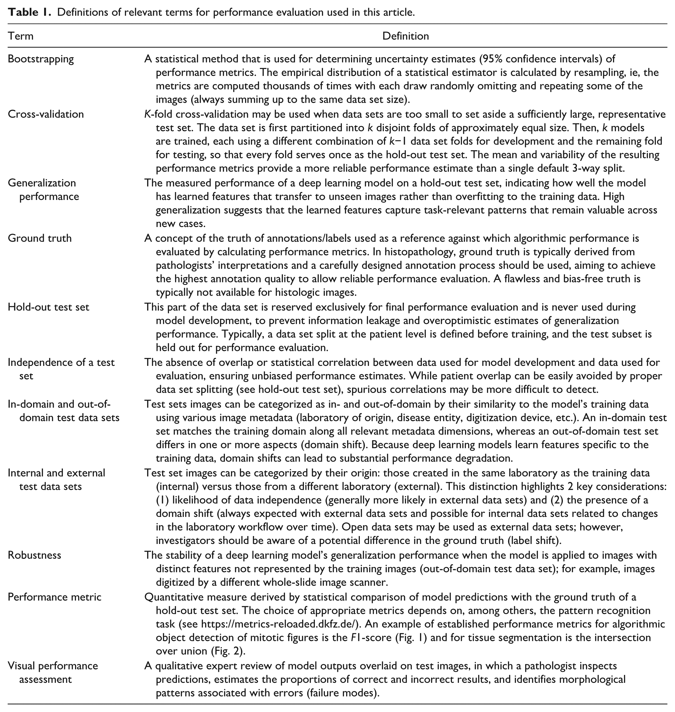
automated image analysis deep learning machine learning performance evaluation testing validation

Artificial intelligence (AI), in particular deep learning (DL), holds great promise for revolutionizing the analysis of microscopic images. Indeed several studies suggest that DL-based automated image analysis (DL-AIA) can improve the accuracy, reproducibility, and/or efficiency of histological evaluations.^8,10,26,69 While there is an increasing body of literature supporting DL-AIA, some veterinary diagnostic and toxicologic laboratories have already incorporated or are considering to implement DL-AIA algorithms into their routine workflows. Similarly, it is expected that researchers will increasingly use these DL tools at a large scale and repeatedly for multiple study populations, not only one-off applications for a standardized study population, to generate biomedical data and gain groundbreaking insights reproducibly across studies. Regardless of these use cases, it is essential to ensure that the quality of DL-AIA is noninferior to traditional methods, as established through qualified performance evaluations.^11,27,33,43 However, due to a lack of recommendations and guidelines, performance evaluation in veterinary pathology is currently conducted with highly variable rigor. As a result, many pathologists remain skeptical about algorithmic performance, are concerned about potential errors, and are uncertain about the extent to which DL-AIA can be trusted when applied beyond the initial proof-of-principle study. The objective of this commentary is to raise awareness about appropriate methods for performance evaluation and validation before its application and to compare advantages and limitations between visual assessment and statistical evaluation. Relevant terms for performance evaluation used in this article are defined in Table 1.

Table 1.

Definitions of relevant terms for performance evaluation used in this article.

Term	Definition
Bootstrapping	A statistical method that is used for determining uncertainty estimates (95% confidence intervals) of performance metrics. The empirical distribution of a statistical estimator is calculated by resampling, ie, the metrics are computed thousands of times with each draw randomly omitting and repeating some of the images (always summing up to the same data set size).
Cross-validation	K-fold cross-validation may be used when data sets are too small to set aside a sufficiently large, representative test set. The data set is first partitioned into k disjoint folds of approximately equal size. Then, k models are trained, each using a different combination of k−1 data set folds for development and the remaining fold for testing, so that every fold serves once as the hold-out test set. The mean and variability of the resulting performance metrics provide a more reliable performance estimate than a single default 3-way split.
Generalization performance	The measured performance of a deep learning model on a hold-out test set, indicating how well the model has learned features that transfer to unseen images rather than overfitting to the training data. High generalization suggests that the learned features capture task-relevant patterns that remain valuable across new cases.
Ground truth	A concept of the truth of annotations/labels used as a reference against which algorithmic performance is evaluated by calculating performance metrics. In histopathology, ground truth is typically derived from pathologists’ interpretations and a carefully designed annotation process should be used, aiming to achieve the highest annotation quality to allow reliable performance evaluation. A flawless and bias-free truth is typically not available for histologic images.
Hold-out test set	This part of the data set is reserved exclusively for final performance evaluation and is never used during model development, to prevent information leakage and overoptimistic estimates of generalization performance. Typically, a data set split at the patient level is defined before training, and the test subset is held out for performance evaluation.
Independence of a test set	The absence of overlap or statistical correlation between data used for model development and data used for evaluation, ensuring unbiased performance estimates. While patient overlap can be easily avoided by proper data set splitting (see hold-out test set), spurious correlations may be more difficult to detect.
In-domain and out-of-domain test data sets	Test sets images can be categorized as in- and out-of-domain by their similarity to the model’s training data using various image metadata (laboratory of origin, disease entity, digitization device, etc.). An in-domain test set matches the training domain along all relevant metadata dimensions, whereas an out-of-domain test set differs in one or more aspects (domain shift). Because deep learning models learn features specific to the training data, domain shifts can lead to substantial performance degradation.
Internal and external test data sets	Test set images can be categorized by their origin: those created in the same laboratory as the training data (internal) versus those from a different laboratory (external). This distinction highlights 2 key considerations: (1) likelihood of data independence (generally more likely in external data sets) and (2) the presence of a domain shift (always expected with external data sets and possible for internal data sets related to changes in the laboratory workflow over time). Open data sets may be used as external data sets; however, investigators should be aware of a potential difference in the ground truth (label shift).
Robustness	The stability of a deep learning model’s generalization performance when the model is applied to images with distinct features not represented by the training images (out-of-domain test data set); for example, images digitized by a different whole-slide image scanner.
Performance metric	Quantitative measure derived by statistical comparison of model predictions with the ground truth of a hold-out test set. The choice of appropriate metrics depends on, among others, the pattern recognition task (see https://metrics-reloaded.dkfz.de/). An example of established performance metrics for algorithmic object detection of mitotic figures is the F1-score (Fig. 1) and for tissue segmentation is the intersection over union (Fig. 2).
Visual performance assessment	A qualitative expert review of model outputs overlaid on test images, in which a pathologist inspects predictions, estimates the proportions of correct and incorrect results, and identifies morphological patterns associated with errors (failure modes).

Why are Proper Performance Evaluations and Validation Important?

When DL models are used by pathologists during routine histological examinations, they are diagnostic tests and have to be validated like any other diagnostic test would. To ensure that the initially defined goals of the DL models are met, performance evaluation is important. This typically includes an, at least, noninferior or even increased diagnostic accuracy, which can be measured and quantified through multiple parameters. High-performance parameters, derived from an extensive and carefully designed evaluation process, provide supportive evidence that the training methods and process were appropriate, and that the final model may be suitable for its intended use case. Since DL model training is an iterative process that uses data to optimize the parameters of a model, the performance of a trained algorithm is highly dependent on many factors such as the training data (including the number of images, image variability, and the quality of the ground truth), the model architecture, and the training process itself (including optimization process, data sampling strategies, and final model selection). Even if all these factors remained the same over multiple training instances, the performance may vary due to the stochastic nature of training (eg, random initialization of weights, random selection, and augmentation of images). Considering all these uncertainties of model development, it is crucial to perform rigorous performance evaluations and to determine the sources of error of the derived model.

The subsequent article will focus on performance evaluation on the level of the pattern of interest (image classification, object detection, and semantic and instance segmentation), whereas we only briefly refer to other relevant evaluation methods considering that they are not specific for automated image analysis. For example, for image classification of tumor malignancy, the question would be if the model had correctly classified all images as benign vs malignant. Performance of an exemplary object detection model for mitotic figures is evaluated by checking if the location of the predictions match with true mitotic figures (Fig. 1).⁸ Segmentation can, for example, be used to measure the size of neoplastic nuclei, and it needs to be ensured that most of the corresponding pixels are correctly predicted (Fig. 2).²⁶

Figure 1.

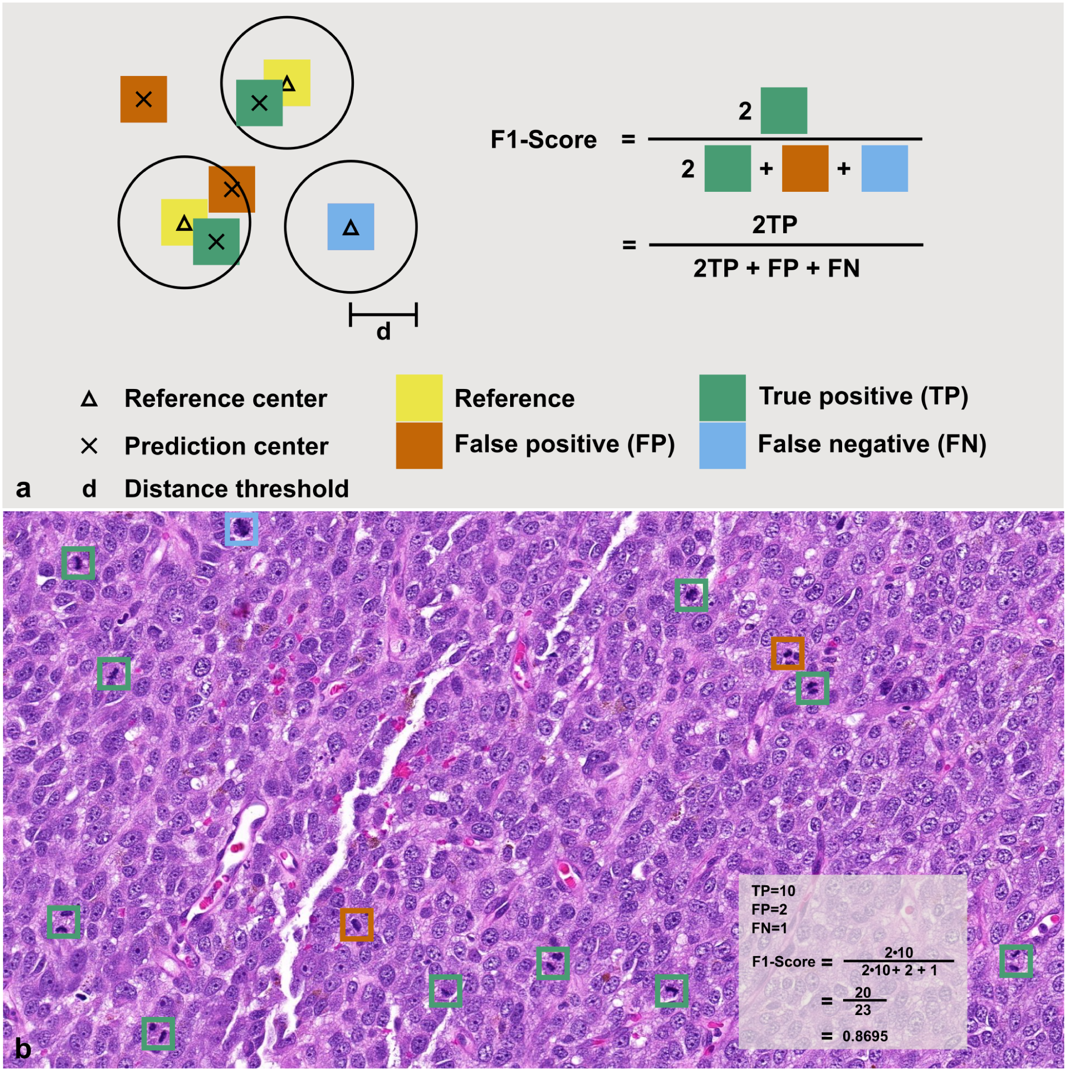
Exemplary performance metric for object detection of mitotic figures using a schematic (a) and real image of a canine oral melanoma (b). Model predictions are compared with a pathologist-provided ground truth and categorized as true positives (TP; the prediction matches a ground-truth annotation; green), false positives (FP, the model detected an object that was not considered a mitotic figure by the annotator; orange), or false negative (FN, the model has missed to detect a mitotic figure labeled by the annotator; blue). True negatives (TN) are not sensible for object detection. With the number of TP, FP, and FN, the F1-score can be calculated, with values ranging from 0 (no successful detection) to 1.0 (perfect performance).

Figure 2.

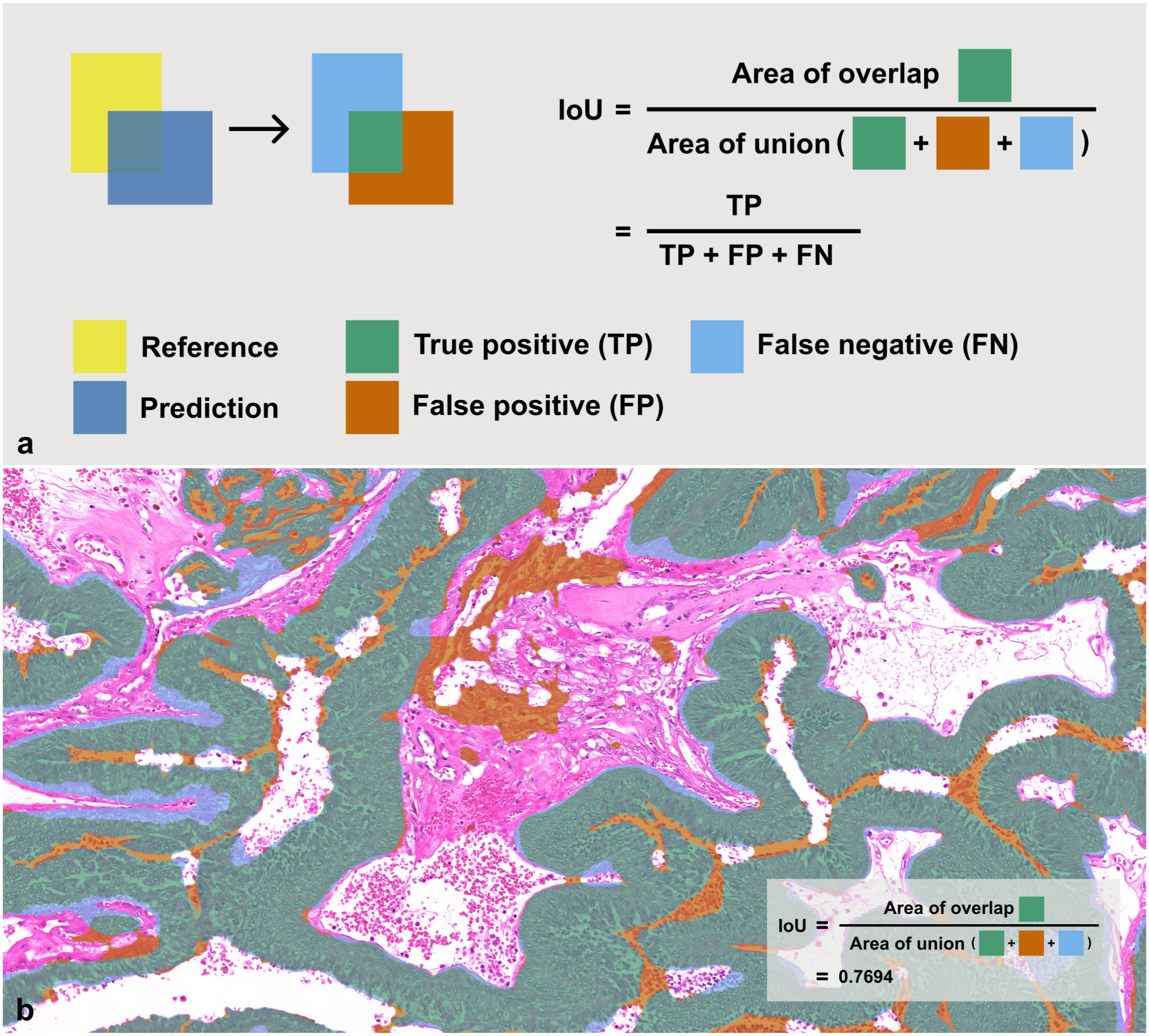
Exemplary performance metric for segmenting tissue components using a schematic (a) and a real image of a canine mammary carcinoma with predictions for neoplastic epithelium (b). Model predictions are compared with a pathologist-provided ground truth, and each pixel is categorized as true positive (TP, green), false positive (FP, orange), or false negative (FN, blue). With the number of TP, FP, and FN pixels, the intersection over union (IoU) can be calculated, with values ranging from 0 (no successful segmentation) to 1.0 (perfect performance).

The performance of a DL model on the pattern level can be evaluated through statistical methods and visual inspection (Table 2).¹¹ Visual evaluation is performed by a pathologist who reviews and interprets algorithmic predictions visualized on the test data set, estimating the proportion of correct and incorrect predictions and identifying the primary sources of error. We are not aware of any published instructions on how to conduct visual assessment. Statistical performance evaluation involves comparing ground-truth annotations (ie, the reference standard) with algorithmic predictions on the test data set, followed by the calculation of performance metrics.^27,43 There are numerous performance metrics that may be used for statistical evaluations of image analysis algorithms. The Metrics Reloaded consortium has assembled a collection of 45 different metrics along with their definitions, pitfalls, and recommendations. The choice of appropriate performance metrics depends on several factors: (1) the pattern recognition task (eg, image classification, object detection, semantic segmentation, or instance segmentation), (2) domain-specific properties (eg, whether the shape or center of an object is relevant), (3) target structure properties (eg, whether objects are of similar or variable size), (4) data set properties (eg, equal class distribution or class imbalance), and (5) algorithm output-related properties.⁴³ A decision guide to find suitable metrics for a specific task is available on the Metrics Reloaded website: https://metrics-reloaded.dkfz.de/. Whereas this article does not discuss the various metrics,⁴³ the distance-based F1-score for object detection tasks will be used in subsequent examples and is therefore explained in Fig. 1. The most commonly applied pattern recognition task is segmentation⁵² (Supplemental Table S2), and an example of a performance metric is given in Fig. 2. In addition to the pattern recognition task, the pathology task should also be considered when selecting metrics. For example, counting tumor cells in an image can be achieved through segmenting nuclei and subsequently counting the predicted objects. For this pattern recognition task, segmentation metrics, such as the intersection over union (IoU), would be the primary evaluation methods for evaluating model performance; however, it would not necessarily indicate how well the model is suitable for the pathology task. Marked under-segmentation of the nuclei (ie, detecting too few pixels of each nucleus resulting in a markedly diminished IoU) could still result in a perfect cell count, whereas slight over-segmentation (ie, connecting 2 nuclei by just a few pixels, thus still resulting in a high IoU) would lead to a reduced cell count. Therefore, evaluating the object detection performance using recall, precision, and the F1-score would be more informative for the pathology task. When using nuclear segmentation for morphometry (ie, measuring nuclear size and/or shape), the IoU might be the more relevant of the 2 metric categories, considering that accurate outlines of nuclei might be more important than overlooking a few nuclei; however, supplemental analyses using object detection metrics certainly provide added value in detecting error modes (eg, detection of false objects with distinct sizes/shapes).

Table 2.

List of different methods for performance evaluation of deep learning-based image analysis algorithms.

Type of Testing	Comparison	Type of Data Set	Main Purpose
Primary Performance Indices
Statistical evaluation	Correctness of algorithmic predictions compared with the ground truth using metrics	In-domain test images^a	Determination of generalization performance to evaluate whether the algorithm can predict the pattern of interest sufficiently well
Statistical evaluation		Out-of-domain test images^b	Evaluation of the performance robustness toward realistic changes in image features (domain shift)
Visual assessment	Pathologist inspection of predictions on test images (eyeballing)	In-domain test images^a	Identification of main sources of error
Visual assessment		Out-of-domain test images^b	Identification of main sources of error related to domain shift
Secondary Performance Indices
Measurement accuracy	Comparison/correlation with other tests (such as pathologists’ scores)	Application data set^c	Evaluation of the consistency to established tests
Biological effect or clinical utility (such as outcome analysis or comparison of treatment groups)	Discriminability of case subgroups (defined through biomedical patient characteristics) by algorithmic predictions	Application data set^c	Evaluation of the reasonableness of the algorithmic application

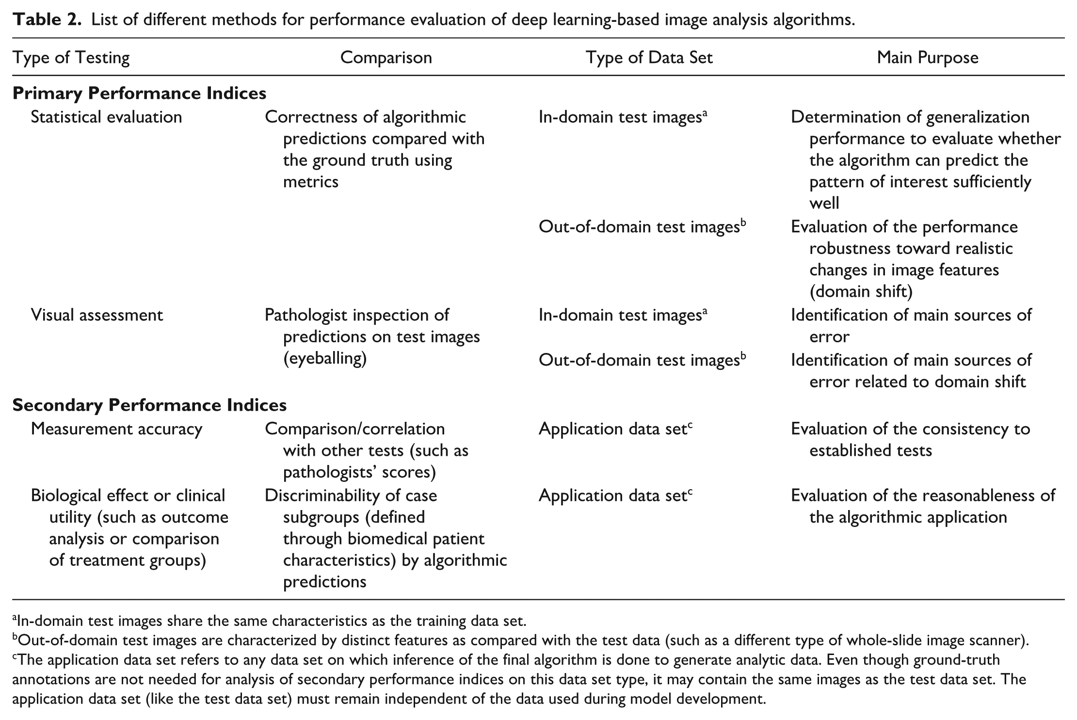
In-domain test images share the same characteristics as the training data set.

Out-of-domain test images are characterized by distinct features as compared with the test data (such as a different type of whole-slide image scanner).

The application data set refers to any data set on which inference of the final algorithm is done to generate analytic data. Even though ground-truth annotations are not needed for analysis of secondary performance indices on this data set type, it may contain the same images as the test data set. The application data set (like the test data set) must remain independent of the data used during model development.

The extent by which the DL model performance should be evaluated depends on many aspects such as the complexity of the model and pattern of interest, the degree of intended investigation (eg, proof-of-concept experiment vs in-depth scientific study), prior evaluation of the model (eg, development from scratch vs transfer to a new laboratory), and the intended application of the DL model (eg, fully automated vs computer-assisted, or one-off research vs routine diagnostics at various laboratories). For example, relatively less rigor may be appropriate for a model developed to count immunohistochemically positive cells for a one-off research application using a specific study set with highly standardized methods of slide preparation. In this case, the model would likely be designed to simulate the interpretation (positive vs negative cell) of a single study pathologist and few uncontrolled sources of error (eg, no differences in the digitization devices) would be expected. In contrast, substantially higher rigor of performance evaluation would be required for a mitotic figure object detection model that is routinely used by multiple diagnostic laboratories across a wide range of tumor types. In that scenario, it would be necessary not only to evaluate whether the DL model can handle various preanalytical variables (eg, different digitization devices), but also to ensure that various pathologists with distinct diagnostic decision thresholds (see below) understand the model’s capabilities and how to interpret its predictions. Given this wide range of required rigor for performance evaluation, we do not make specific recommendations in this article as to which method is required as a minimum standard; instead, we explore methods suitable when requirements for high-performance evaluations are imposed. These considerations are summarized in Supplemental Table S1.

For proper performance evaluation, a fundamental understanding of the concept of machine learning is critical. Investigators need to be aware that inappropriate DL techniques can create models that are remembering the data they were trained on (overfitting) or learn unintended, spurious correlations between “simple” patterns of the training images with the output (shortcut learning) instead of learning the complex decision criteria needed to perform the desired pathology task.³⁰ An example for shortcut learning of models is if it learns to identify malignant tumors by the presence of ink at surgical margins and benign tumor by the lack thereof (ie, the unintentional correlation that margin evaluation may be done more commonly in aggressive tumors), instead of recognizing the diagnosis by malignancy criteria, such as nuclear pleomorphism. A slightly more complex spurious correlation could arise for a model that was developed to classify mammary adenoma versus carcinoma in dogs and cats, whereas slides from dogs were digitized with one scanner and slides from cats with a second scanner. While cats have a higher frequency of mammary carcinoma as compared with dogs, the model may falsely learn to correlate simple features, that are characteristic of the second scanner (color representation, depth of field, etc.), with malignancy. Independent data sets used separately for training and testing, defined by the absence of overlapping cases and spurious correlations, are the only way to distinguish these effects. For this reason, it is considered mandatory to evaluate performance on independent hold-out test data sets.^11,33 Unfortunately, spurious correlations may be much more subtle than in the 2 examples above,³⁰ and may not be obvious to the human eye. Consequently, it can be challenging to ensure data independence; the least that must be done is a data set split on the patient level (ie, images from the same patient are not part of the different data subsets).

To illustrate the relevance of an independent data set split during model development, let us make a comparison to the veterinary pathology residency program. Analogous to the model development phases of (1) training, (2) validation, and (3) testing (Supplemental Figure S1, see previous publications for more details^13,39), a resident will (1) study their notes, (2) take mock exams (formative assessment), and (3) sit the final certification examination (summative assessment), respectively. In preparation for the board examination, a resident will reread study materials until they hope they have mastered the content. A mock exam reveals whether the resident is ready to take the certification exam or would benefit from further study iterations (if time allows). Passing the board examination certifies the candidate as a Diplomate of Veterinary Pathology, indicating that she/he can solve pathology tasks with high accuracy. To ensure the resident has understood and can apply principles and concepts, the board examination questions must be kept confidential and distinct from study materials (eg, it is prohibited to use mock exams or old exam questions). In other words, the test set must remain independent of the training and validation sets. If the board examination questions overlapped with the mock exams, job readiness would be overestimated. Similarly, test performance of DL models is inflated when there is any overlap (data leakage) between training, validation, and test data sets. A resident might engage in shortcut learning if, for example, a supervisor places the correct answer of multiple-choice questions in option C most of the time. While the student can readily understand the supervisor’s pattern of formulating a question, the perceived resident’s knowledge by the supervisor will be misleading. For determining the level of knowledge reliably, this unintended cue (similar to spurious correlations of data sets) must be avoided in the board examination, for instance, by randomizing the answer option order. In summary, exam and test data set construction both require high attention to avoid bias that would overinflate or underscore performance.

These independent test data sets can be further classified into “in-domain” and “out-of-domain.”^11,51 The in-domain test set has similar image characteristics to the images used for training the model, ie, it is typically produced alongside the training data set but separated as a hold-out set before initiating training. This means that the included images from the training and test set are derived by the same tissue types, disease entities, slide preparation methods (same batches), digitization devices, etc., but from an independent study population (patients). Evaluating performance on the in-domain test set allows to establish the generalization performance of the DL model to new cases, ie, whether the model learned features that are relevant to almost exclusively identify the pattern of interest or whether the features overlap with other patterns (ie, too many false positives) or are too narrow (ie, too many false negatives).⁴⁹ Generalization performance is measured by calculating the number of algorithmic predictions that are correct or incorrect, similar to the score of a pathology resident in the board examination. Testing on images from independent patients (ie, that were not used for training) will indicate whether the model learned spurious correlations or just remembered the training data. A detailed error analysis helps to identify common failure patterns, where the model missed learning discriminatory features, or mistakenly learned features that are unsuitable for discrimination of the patterns of interest.

An out-of-domain data set, on the contrary, has distinct image features compared with the training data set, which may cause a so-called “covariate domain shift” in the image representation (ie, the distribution of the model inputs shifts from training to test). Using the residency training example from above, let us imagine the resident was trained exclusively with histologic slides from mammals, and during the certification examination she/he has to evaluate a histological section from a bird for the first time. The low magnification pattern of increased nuclear density in this avian slide due to the nucleated red blood cells may lead to a false interpretation of inflammation, which would be a reasonable inference on mammalian slides but not on avian tissue. Algorithms learn much more subtle domain-specific features from the training data set, and subsequently may fail to identify the pattern of interest in test images from a distinct domain.^2,3,13 Domain changes may be related (with varying impact on model robustness) to animal species, disease conditions/entities, case inclusion/exclusion criteria, sample processing (eg, longitudinal vs transverse orientation of the organ during trimming), sectioning thickness, staining composition (batch effect or interlaboratory variability), different digitization devices (whole-slide image [WSI] scanner company and type), digitization settings, or image processing.^2,3,61 The challenge is that the learned features of a DL model do not necessarily simulate the perception of pathologists and, therefore, the relevance of the domain shift on performance is often not obvious without formal testing. For example, the difference between 2 whole-slide image scanners may be primarily interpreted by a pathologist as a variable color profile, whereas DL models typically pick up several additional scanner-specific features. Subsequently, techniques that address these color profiles, such as color augmentation during training or image normalization, do not fully restore the model’s generalization performance on an previously unseen WSI scanner.^2,3 Following this discussion, it can generally be assumed that image data sets generated by different laboratories (“external” data) exhibit a certain degree of domain shift. Changes within one’s own laboratory workflow, such as acquisition of a different WSI scanner, can also induce a relevant domain shift for “internal” image sets. To determine whether a data set is to be considered in-domain or out-of-domain, it is critical to collect and document all relevant image metadata.

Testing performance on the out-of-domain data set primarily evaluates the robustness of the model, ie, whether the learned features are also relevant to other image domains or are overly specific to the training domain. This information is critical when models are intended for widespread use in multiple laboratories or diagnostic settings. However, even if sufficient performance of a model on out-of-domain data was shown, it is worth noting that each data set only covers a part of real-world data diversity. Even if generalization in multiple domain-shift scenarios was shown, this does not guarantee robustness for every case. Thus, it is recommended that every laboratory should ensure that the DL-AIA algorithm is appropriate for their actual “real-world” data.²⁷ A second benefit of an out-of-domain data set is that it is more reliable since it is less prone for spurious correlations with the training data, and out-of-domain testing may therefore be valuable, even if the model is only intended for a narrow applications, for reinsuring sufficient generalization performance.

Besides performance measures on the level of the pattern of interest as described above (eg, the model detects 10 of 11 ground-truth mitotic figures and detects 2 nonmitotic figures resulting in an F1-score of 0.870; Fig. 1), performance can additionally be indirectly judged on higher levels that reflect the diagnostic application of the model (secondary performance indices). One example would be the measurement level; following the example above, the algorithmic mitotic count is 12, while the pathologist’s count is 11 with an absolute error of 1. Errors or consistency with traditional evaluation methods (ie, pathologists’ counts) can be further evaluated, for example, by scatterplots or correlation analysis. Another secondary indicator would be to evaluate whether the algorithmic mitotic counts can discriminate between patients with tumor-related death and those who survive (survival analysis). The type of error should also be judged in context of the clinical consequences; for example, a classification model that misclassified a benign tumor as another benign tumor type may have a minor impact on the treatment decision, whereas misclassification as a malignant tumor would markedly alter treatment.

Whereas the abovementioned primary and secondary performance measures are often conducted for the “preclinical” evaluation, which is done in conjunction with model development, DL-AIA algorithms need to be further validated when implemented into the laboratory workflow (“clinical validation”).^27,51 While these further validation steps are beyond the scope of this article, we want to highlight some additional considerations that are relevant for a reliable use of DL-AIA. These considerations include the performance on real-world data of the specific laboratory, computational efficiency of the model, suitability of user interface and model output (visualization), bias in human-computer-interaction, establishment of standard operating procedures for AIA usage, user training, and ongoing quality management.^27,51,58

Why is Performance Evaluation Challenging?

DL-AIA models are developed to overcome diagnostic challenges of the current workflow, which includes limited time availability of pathologists for quantitative measurements; shortcomings in diagnostic accuracy, for example, by only using a categorical test instead of a numerical test; and low interobserver reproducibility. For the latter 2 objectives, a superior model performance, in comparison with a pathologist’s evaluation, is intended, which can be quite difficult to demonstrate considering the challenges to establish a perfect ground truth that is used as an output during model training and as a reference standard for performance evaluation. For most patterns of interest, pathologists are considered the gold standard, but humans are prone to various biases that challenge impartial assessment.¹ Thus, inaccuracy and inconsistency in the ground-truth labels can hardly be avoided.^12,25,68 Consequently, most models are developed and tested with an imperfect ground truth while the model developers aim at outperforming this reference standard, resulting in a catch-22 situation (Fig. 3). Even if a DL model would perfectly simulate the annotator’s decision threshold, the performance evaluation would still indicate some errors, which, in reality, would be random errors in the ground truth of the test set rather than algorithmic errors. Only rarely can a truly superior gold standard be established, such as when histological images are classified based on their molecular signatures.⁵⁴

Figure 3.

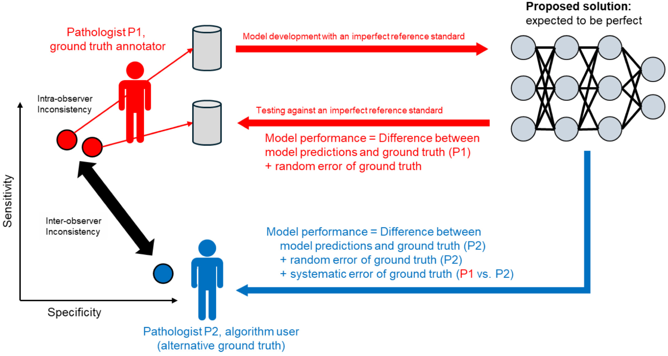
Catch-22 situation of deep learning-based model development and testing. One of the diagnostic problems that a deep learning model may be expected to overcome is the interobserver inconsistency (mainly systematic errors) and intraobserver inconsistency (mainly random error) of pathologists’ interpretations. The systematic error between 2 pathologists may lead to distinct sensitivity-specificity thresholds in their decision. For example, one pathologist may have a relatively high sensitivity and low specificity with high intraobserver consistency (two red dots); however, there are still random errors, such as overlooking an object of interest or an arbitrary decision of borderline morphologies. A second pathologist may have a low sensitivity, but high specificity (blue dot). Despite this well-known difference in pathologists’ interpretations, they are paradoxically defined as the gold standard and these types of error can be expected to be present, to a certain degree, in the established reference standard for model development and testing (ground-truth data set). An unbiased and flawless truth is typically not available for histological images. As a model is trained with imperfect data and, more importantly, is evaluated against an imperfect reference, it becomes challenging to demonstrate superiority of the model in diagnostic accuracy as compared with the pathologist. Performance of the final model (as defined by a qualified performance metric) is determined by calculating the discrepancy between algorithmic predictions and the pathologist’s ground truth, whereas even a perfect model would have less than 100% performance due to random errors in the ground truth. Based on the red pathologist’s decision thresholds, the resulting model is expected to be rather sensitive and less specific. To complicate matters further, a second pathologist (blue, in this case the more specific observer) may criticize the algorithmic performance due to a perceived low specificity of the model. However, this difference in the performance perception is primarily related to the differences between the 2 raters (ie, the systematic error of the ground truth); precisely, the issue the model was developed to address in the first place. This potential catch-22 situation emphasizes the need for high-quality data sets, thorough performance evaluation methods, and careful performance interpretation.

Another highly relevant challenge is the marked interobserver differences in pathologists’ interpretations, particularly regarding the setting of thresholds between label classes or between patterns of interest versus imposters.^{8,10,26,68,69} An algorithm is likely to reflect all biases of the training data, including the individual decision threshold applied by the data set annotator. However, if the algorithm is used by another pathologist with a differing individual decision threshold, an unjust perception of poor algorithmic performance may arise, which, mostly reflects the mismatch between the 2 pathologists (ie, a systematic difference between the model user and data set annotator) and not necessarily the incapability of the DL model (Fig. 3). In our experience, pathologists often expect perfection from DL models while remaining unaware of their own variability to other pathologists, which may not have been accounted for in the training data set’s ground truth.

To support our claims about intrarater and interrater inconsistencies, this paragraph and the next provide examples from published literature. These findings intend to show that some microscopic patterns are extremely difficult due to substantial morphological overlap with look-alikes, which is coupled with different thresholds between observers in discriminating between patterns of an object and an imposter. While numerous studies have demonstrated the challenges of reproducibility in quantitative pathology tasks, the 3 examples below also illustrate how annotation variability can influence the performance evaluation of DL models. These 3 studies, evaluating an object detection task, used the F1-score as the metrics for performance evaluation, which is the harmonic mean of precision (also known as positive predictive value) and recall (also known as sensitivity) with values ranging from 0 (no successful detection) to 1.0 (perfect performance; Fig. 1). In the first study, object detection models for mitotic figures were evaluated using the open access data set from the TUPAC16 challenge with annotations by the initial data set creators and an alternative ground truth established by a second research team.¹² A comparison of the 2 data sets revealed that both included labels for the same 1239 objects, while 313 and 760 objects, respectively, were unique to one data set. When the same DL model development approach was applied, the measured performance ranged from an F1-score = 0.549 to 0.735, solely depending on which ground-truth definition was used. The second study applied a similar mitotic figure detection model, which had been shown to have a high performance on the study population (immunohistochemistry-guided ground truth) with an F1-score of 0.83.⁸ Twenty-three study pathologists evaluated the same images and counted between 1263 and 4412 mitotic figures (ie, they differed by a factor of up to 3.5). Their performance in relation to the ground truth ranged between F1 = 0.53 and 0.79, with some being highly consistent with the DL model and others having markedly differing decision thresholds (either more sensitive or more specific). These pathologists with distinct decision thresholds are likely to be skeptical about algorithmic performance, even though the model is more consistent with the ground truth than their interpretation threshold.

The third study developed an object detection model for binucleated cells in mast cell tumors.⁹ To establish a benchmark for algorithmic performance, 6 pathologists annotated binucleated cells in a small subset of the test set. Compared with the ground truth, which was established by a different annotator with a total of 148 ground-truth annotations, the 6 pathologists additionally annotated between 56 and 542 objects. Depending on which truth was used for testing the model (majority vote of benchmark pathologists or the initial single annotator ground truth), the measured performance of the same model varied between an F1-score of 0.424 (majority vote) to 0.667 (initial ground truth). On the initial ground truth, the benchmark pathologists achieved an F1-score between 0.270 and 0.526. If the pathologists with the lower metric values evaluate the model’s performance it would be their impression that the model had overlooked numerous binucleated cells, whereas this biased interpretation would be related to the lower decision threshold (ie, higher sensitivity) of these pathologists as compared with the ground truth and DL model.

From a statistical perspective, the limitations of the reference standard can be conceptualized as 2 forms of uncertainty: aleatoric and epistemic.³⁵ Aleatoric uncertainty reflects inherent ambiguity in the data, such as genuine morphological overlap between patterns of interest and imposters, where even highly experienced pathologists may reasonably disagree. Epistemic uncertainty, in contrast, arises from incomplete knowledge or suboptimal processes, such as poorly defined diagnostic criteria, inadequate training, or inconsistent annotation protocols. Both uncertainty types are embedded in the ground truth used for DL model development and testing, and they jointly determine the “noise level” of the labels. Due to this label noise, even a conceptually perfect model may be unable to reach an apparent performance of 100% relative to the reference standard, because some fraction of apparent “errors” are in fact disagreements with inconsistent or ambiguous labels rather than genuine algorithmic failures.

Quantifying this label uncertainty is important for placing DL-AIA performance into context. Such a benchmark can be either defined by comparison of the consistency of the annotation workflow or by multi-rater studies. Consistency of the test set ground truth can be determined if the same annotation workflow is applied a second time to the test set images. The difference between the labels of the 2 data sets will be a good indication of random error/aleatoric uncertainty and thereby approximate an upper bound on achievable algorithmic performance. For example, if the agreement on the object-level between the 2 time points is F1 = 0.8, then it is unreasonable to expect a DL model applied to the same labels to substantially exceed this agreement. In such settings, a model achieving an F1-score close to the level of agreement may already represent near-optimal performance, even though the metric itself appears far from perfect. Multi-rater studies, in which several pathologists independently annotate the images of the test set and are compared with the ground truth, can be used to estimate the interrater reproducibility of the reference standard and thereby approximate the systematic erro/epistemic uncertainty. Interrater agreement statistics (eg, pairwise F1-scores, Kappa coefficients, or majority-vote comparisons) may provide an estimate of the lower performance boundary for the model to be noninferior to pathologists.

These considerations emphasize that performance metrics must always be interpreted relative to the quality and consistency of the ground truth. When reading DL-AIA studies, it is therefore essential to consider how the reference standard was created (eg, single annotator vs consensus or majority vote)¹³ and whether any estimates of interobserver or intraobserver variability are available. Ideally, studies should report both human-ground-truth and model-ground-truth agreements on the same test images, allowing the reader to judge whether the algorithm has reached, matched, or exceeded typical expert consistency for the task at hand. Without this benchmark, a performance metric such as F1-score of 0.7 remains difficult to interpret; it may indicate poor performance on a simple, highly reproducible task or, conversely, very strong performance on a task for which human agreement is intrinsically limited by high aleatoric uncertainty. A complementary approach to interpretation, if model performance is sufficiently high, is to determine the biological effect or clinical utility of its measurements (eg, whether algorithmic mitotic counts from tumor sections are capable of discriminating patient outcomes). The biological effect or clinical utility of algorithmic measurements should be evaluated in comparison with the traditional method (typically pathologists’ counts or scores), to reliably interpret the extent of the effect.

Current Practice of Performance Evaluation

Currently, there are no established guidelines in veterinary pathology regarding when and how to apply methods of statistical and visual performance assessment. Therefore, this section analyzes current practices in research articles published in selected veterinary journals. A literature search was conducted on the websites of 5 journals focusing on veterinary pathology using the following search terms: “artificial intelligence,” “machine learning,” and “deep learning.” Original articles published between 1 January 2015 and 9 March 2025 that describe the development of DL-based models for microscopic images (histology and cytology, histochemical stain, and immunohistochemistry) and/or the evaluation of such a DL model’s performance on any of the levels listed in Table 2 were included. We identified 25 articles in Toxicologic Pathology,^{5,7,17,18,20,24,29,31,34,36–38,41,46–48,50,53,55,56,59,60,65,66,70} 6 articles in Veterinary Pathology,^{8,10,23,26,54,69} and no eligible articles in the Journal of Comparative Pathology, Veterinary Clinical Pathology, and Journal of Veterinary Diagnostic Investigation. From these articles, we extracted information on (1) the type of AI utilization, as defined for the Veterinary Pathology reporting guideline;¹¹ (2) the use of different data set types for performance evaluation, as defined by a recent review article;¹³ (3) the independence of the data sets used for performance evaluation from the development data set; and (4) if visual and statistical performance evaluation was conducted (Supplemental Table S2).

Of the 31 eligible articles, most (N = 30) had developed new DL models for their studies, either for a previously unexplored use case (N = 28) or using an established development process for the use case (N = 2). Only one study validated a previously published DL model on a second test set; this study will not be further discussed here. The 30 studies that developed new models used a primary data set with ground-truth annotations for development of the DL model (N = 30) and performance testing (N = 19, 63%). In addition, performance evaluations were done on secondary test sets (data set with ground-truth annotations created independently from the primary data set) in 3 instances, 2 of which did not use a primary test data set, and an application data set (data set without ground-truth annotations, but with biomedical metadata of patients) in 15 instances. The test data sets of 4 studies are publicly available.^10,23,26,69

For the 21 studies that used a primary or secondary test data set with ground-truth annotations, the test set was considered independent in 12 instances (57%), while concerns for data leakage (ie, use of image parts from the same patient in both the development and test subsets) was raised for 9 articles (43%; Fig. 4). Visual performance assessment was reported in 18/21 studies (86%, not possible in 2 studies as image classification was used) and statistical performance metrics could be found in 18/21 studies (86%), with a benchmark of pathologists’ performance as compared with the ground truth being available in 5 studies. Secondary performance indices (determined on any data set type) were additionally provided in 15 studies (71%).

Figure 4.

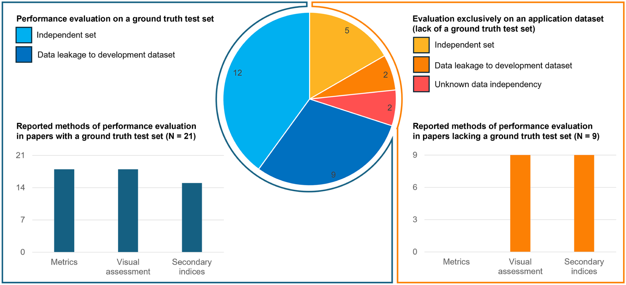
Current practice in performance evaluations across 30 studies published in the journals Veterinary Pathology and Toxicologic Pathology. The pie chart in the center shows the proportion of studies that did (blue) or did not (yellow to red) use a ground-truth test set. The bar charts summarize the performance evaluation methods reported by these 2 groups of papers.

Studies that did not utilize a test set with ground-truth annotations (N = 9/30, 30%), restricted their performance evaluations on application data sets to visual assessments (N = 9), in many cases by providing exemplary histologic images with overlays of algorithmic predictions in their articles, and secondary performance indices (N = 9). For these application data sets, concerns of data leakage were found in 2 studies, whereas 2 studies lacked information to judge data independence. Terminology used to describe the pathologists’ interpretation of the visual assessments included “satisfactory,” “adequate,” “suitable,” “frequently failed,” and “occasionally missing.” This evaluation approach was done in 9/25 (36%) of the articles published in Toxicologic Pathology, which aligns with a survey of toxicologic pathologists that revealed that 40% of respondents exclusively relied on visual performance evaluation by a single pathologist when developing DL models.⁵²

The data set creation and image inclusion methods (reported in 24/30 studies) followed 2 broad approaches: (1) a priori to model training and (2) stepwise during model training (active learning-like). An a priori data set creation had almost always (N = 14/15, 93%) resulted in a separate test data set with ground-truth annotations (Supplemental Figure S1), and 12/15 studies leveraged this test set to calculate statistical performance evaluations. One study create ground-truth annotations a priori for the development data set; however, not for the test set.¹⁸ Instead, algorithmic predictions on each image tile of the test set were presented to a pathologist, who verified if they were correct of false.¹⁸ Whereas this approach can be used to calculate performance metrics, a form of anchoring or confirmation bias of the annotator should be acknowledged.⁵⁷ Stepwise data set creation was done by 8 studies and was motivated by higher time-efficiency, since this approached relied on the minimum number of annotations needed for training sufficient performant algorithms. This approach is characterized by cycles of annotation creation, model training, preliminary model inference, and visual quality assessment (Supplemental Figures S2 and S3). In each cycle, the training data are augmented by new images and annotations (computer-assisted annotation method) with subsequent continuation of training of the preliminary models. The preliminary models’ predictions are used in guiding the developer to select particularly challenging images (active learning-like method) and are often used to speed up labeling (computer-assisted annotation method). Whereas ground-truth annotations are always needed for model training, 5/8 studies (63%) had not reported establishment of a test set with ground-truth annotations, consistent with a 2021 survey of toxicologic pathologists that found 21% of respondents did not perform data splitting into training, validation, and test sets.⁵² Possibly related to the time-efficient concept, this active learning-like workflow seems to be often associated with avoiding the creation of laborious annotations of a test set. When establishing a test set, it is important that the data set split is done from the initial data set and not included in the stepwise model / data set creation.

Comparison of Statistical and Visual Performance Evaluation

In veterinary pathology, there is currently no consistent approach to evaluate the performance of DL models. Some authors rely exclusively on visual assessment, presumably to eliminate the time investment required for test data set creation, while others provide statistical analyses (see above). In human medicine, clear recommendations exist from the College of American Pathologists, which mandate rigorous statistical performance evaluation for all DL-AIA algorithms before their implementation as diagnostic tools for patient samples.²⁷ Similarly, the Veterinary Pathology reporting guideline for research studies on AI-based AIA recommend the use of statistical evaluations in publications unless authors can provide a rational explanation for why metrics are not applicable.¹¹ This reporting guideline emphasizes that the advantages of statistical performance evaluation will, in most research projects, outweigh the time investment required for data set creation. However, detailed recommendations for ensuring sufficient performance of diagnostic DL-AIA algorithms for the various veterinary applications are currently lacking. We encourage the veterinary pathology community to engage in further discussions on this topic. To raise awareness and establish a foundation for good scientific practices in our field, this section compares the advantages and disadvantages of visual and statistical performance evaluation approaches (Table 3).

Table 3.

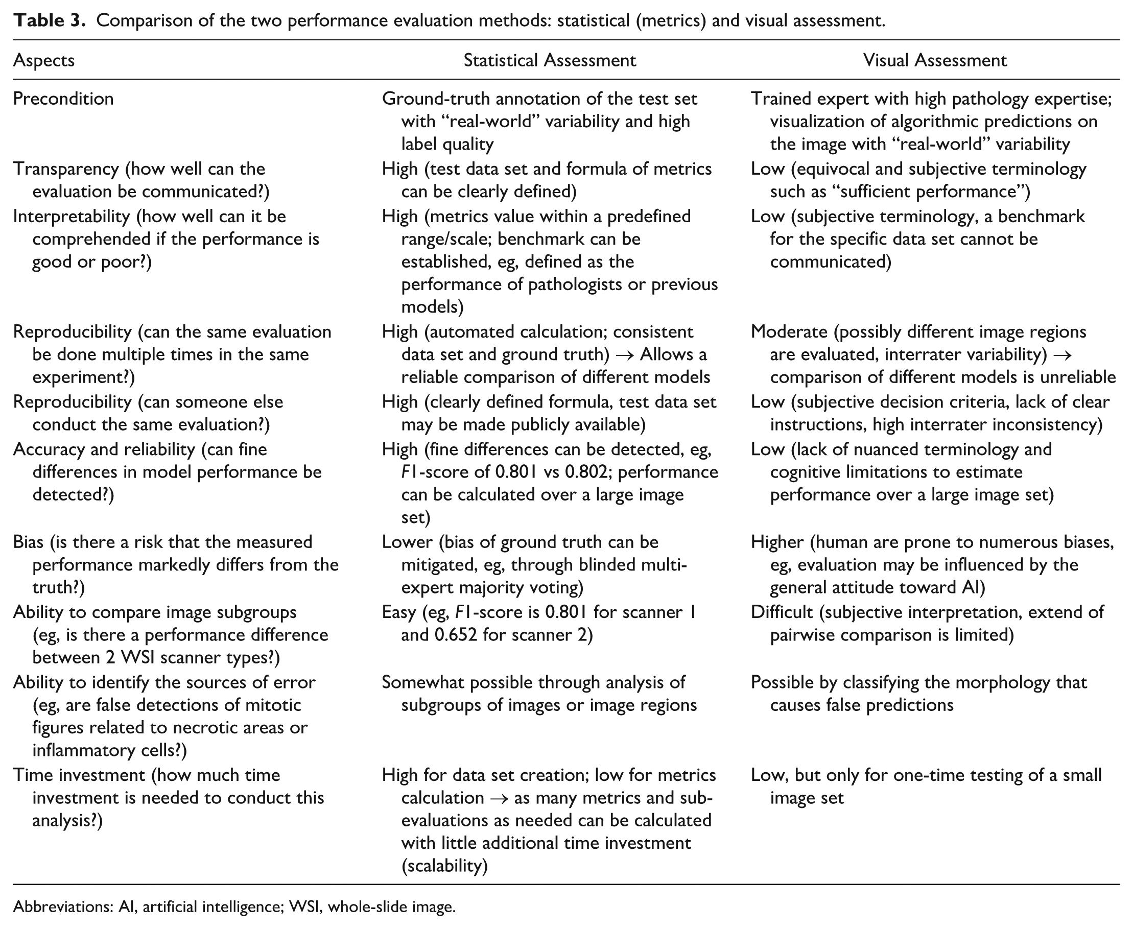
Comparison of the two performance evaluation methods: statistical (metrics) and visual assessment.

Aspects	Statistical Assessment	Visual Assessment
Precondition	Ground-truth annotation of the test set with “real-world” variability and high label quality	Trained expert with high pathology expertise; visualization of algorithmic predictions on the image with “real-world” variability
Transparency (how well can the evaluation be communicated?)	High (test data set and formula of metrics can be clearly defined)	Low (equivocal and subjective terminology such as “sufficient performance”)
Interpretability (how well can it be comprehended if the performance is good or poor?)	High (metrics value within a predefined range/scale; benchmark can be established, eg, defined as the performance of pathologists or previous models)	Low (subjective terminology, a benchmark for the specific data set cannot be communicated)
Reproducibility (can the same evaluation be done multiple times in the same experiment?)	High (automated calculation; consistent data set and ground truth) → Allows a reliable comparison of different models	Moderate (possibly different image regions are evaluated, interrater variability) → comparison of different models is unreliable
Reproducibility (can someone else conduct the same evaluation?)	High (clearly defined formula, test data set may be made publicly available)	Low (subjective decision criteria, lack of clear instructions, high interrater inconsistency)
Accuracy and reliability (can fine differences in model performance be detected?)	High (fine differences can be detected, eg, F1-score of 0.801 vs 0.802; performance can be calculated over a large image set)	Low (lack of nuanced terminology and cognitive limitations to estimate performance over a large image set)
Bias (is there a risk that the measured performance markedly differs from the truth?)	Lower (bias of ground truth can be mitigated, eg, through blinded multi-expert majority voting)	Higher (human are prone to numerous biases, eg, evaluation may be influenced by the general attitude toward AI)
Ability to compare image subgroups (eg, is there a performance difference between 2 WSI scanner types?)	Easy (eg, F1-score is 0.801 for scanner 1 and 0.652 for scanner 2)	Difficult (subjective interpretation, extend of pairwise comparison is limited)
Ability to identify the sources of error (eg, are false detections of mitotic figures related to necrotic areas or inflammatory cells?)	Somewhat possible through analysis of subgroups of images or image regions	Possible by classifying the morphology that causes false predictions
Time investment (how much time investment is needed to conduct this analysis?)	High for data set creation; low for metrics calculation → as many metrics and sub-evaluations as needed can be calculated with little additional time investment (scalability)	Low, but only for one-time testing of a small image set

Abbreviations: AI, artificial intelligence; WSI, whole-slide image.

While visual performance evaluation is only time-efficient when done nonexhaustively on a small image set for a few times, it has several limitations compared with statistical methods, primarily due to the subjectivity inherent in expert assessments. Criteria of what constitute the different performance levels for subjective visual assessment cannot be defined transparently and reproducibly. Communicating the results of visual evaluations is therefore restricted to subjective terminology, such as “sufficient” or “suboptimal.” In contrast, statistical evaluation requires a ground-truth data set, which is time-consuming to create, but it enables extensive and repeated analyses with minimal additional time investment (scalability). Statistical evaluation produces specific performance metrics, such as an F1-score (eg, F1 = 0.801), based on clearly defined formulas. Thus, these metrics are unambiguous and can be easily reproduced by other algorithm developers.

The main advantage of visual performance evaluation is its ability to identify the sources of algorithmic error by visual inspection of algorithmic predictions on the images, which is possible for object detection and segmentation tasks, but not for image classification or regression tasks. A trained pathologist can detect shared features of false predictions and rank error sources accordingly. For example, a pathologist might observe that a mitotic figure detection algorithm produces many false positives in inflamed or necrotic areas, suggesting that the training data set should be augmented with these regions or that such regions should be excluded for model application. However, statistical metrics can complement this process by narrowing down the images worth investigating visually, as they can display results on a per-image or subgroup basis. Statistical evaluation also has the potential to detect “hidden stratification” within test data sets.³³ For instance, a test data set comprising images from multiple WSI scanners may reveal, through stratified analysis, that images from a particular scanner performs poorly, making it unsuitable for use with this particular algorithm.^2,3

Both visual assessment and ground-truth annotations are prone to human bias, but the extent of bias can be minimized in ground-truth annotations using sophisticated methods, such as blinded majority voting by multiple annotators.⁶⁸ In contrast, visual assessment is more susceptible to bias, which can significantly influence performance evaluation for complex patterns of interest. For example, AI enthusiasts may unconsciously overestimate performance by ignoring errors, while AI skeptics may underestimate performance by focusing excessively on errors. In addition, the threshold for acceptable performance may decline over time as developers invest significant effort into model development, even if performance improvements are negligible. Statistical evaluation, on the contrary, is entirely reproducible when using the same test data set and ground-truth annotations. While statistical evaluation can be applied to large data sets (encompassing a real-world variability), visual assessment is often restricted to few selected image regions. This limitation introduces the risk of evaluating a nonrepresentative subset of regions. Even if large image regions or multiple images are assessed visually, it is cognitively challenging to estimate average performance across a vast number of decisions.

A significant limitation of visual assessment is its inaccuracy when comparing different models or training approaches. The low number of image regions that can be compared pairwise and the cognitive limitations of humans, such as estimating the proportion of over-segmented tissue, make such comparisons unreliable.¹ In contrast, statistical performance metrics enable a finely nuanced differentiation of model performance. However, the choice of a specific metric can influence the ranking of models. To address this, the use of multiple complementary metrics is generally recommended.^42,43 For selection of the proper performance metrics for the specific task, we refer to the Metrics Reloaded website: https://metrics-reloaded.dkfz.de/.

To properly interpret the performance of a DL-AIA algorithm, a benchmark established for the specific test images is essential. However, benchmarks can only be accurately defined using metrics (ie, when compared against the ground truth of the test set), and cannot be derived from subjective visual assessments. Without a benchmark, it is difficult to determine whether a performance metric, such as an F1-score of 0.7, is good or bad, as this depends on factors such as data set composition (eg, the proportion of difficult cases and image quality), task complexity, and ground-truth consistency. While perfection of a DL model is not expected, the goal should be to demonstrate improvement over previous tests. This improvement can be defined in 2 ways: (1) using traditional tests (eg, assessments by multiple pathologists) to set a minimum performance threshold^{8,10,23,26,69} or (2) by outperforming a state-of-the-art model through optimization of the model development process.^2,3 When test data sets and their ground-truth annotations are publicly available, the superiority of a DL model can even be compared across multiple studies. However, care must be taken when applying a model to an external public data set (ie, created by a different group), as performance differences may arise not only from a domain shift but also from differences in ground-truth definitions (label shift).^3,12,68

Requirements of the Test Data set

The precondition for performance evaluation is the availability of a data set subset reserved for testing (hold-out test set). Due to the delicacy of performance evaluation, creation of the test set has particularly high requirements for both image quantity and label quality, which are discussed in this section.

First, it is critical that the test set is not used for training or model optimization (such as hyperparameter tuning).^11,33 To ensure that the features learned by a DL model are generally useful for predicting the pattern of interest, generalization performance must be evaluated on a previously unseen hold-out test data set (ie, images from the same patient must not be distributed across data subsets).^11,33 During training, a model may overfit to the training data, possibly learning highly specific features of those images. If such an overfitted model is tested on other parts of the same images used for training (data leakage), it may exhibit seemingly high performance.¹⁶ However, this performance is misleading, as it is driven by spurious correlations in the test images and cannot be reproduced on an independent test set (ie, later model application). Concerns about data leakage were identified in some previous publications (see above). However, even with a data set split on the patient level, data dependencies cannot be fully excluded (eg, all tumor slides have inked margins while slides with nonneoplastic lesions lack ink). Risk for data bias can be reduced when training images and testing images are created in separate batches (possibly use a second test data set created by the same group at a later time point) or at different laboratories using external images. Consequently, it is advisable to evaluate models on multiple test data sets (primary and secondary) before routine usage.

Careful consideration should be given to the size of the test data set, as this directly affects the precision and reliability of the performance estimates. In many DL-AIA studies, test set size is driven primarily by data availability or annotation capacity.³³ However, even simple sample size considerations can help to avoid overinterpretation of unstable metrics. For example, a mitotic figure detection algorithm with an F1-score of 0.9 based on a small number of cases may appear excellent, yet the corresponding confidence interval could be so wide that substantially lower “true” performance cannot be excluded. In contrast, a similar point estimate derived from a sufficiently large number of independent cases will have a much narrower confidence interval and therefore provide stronger evidence that the performance is acceptable for the intended diagnostic application. From a practical perspective, test set size planning can be framed in terms of the desired precision of key metrics, rather than formal hypothesis testing or statistical power calculations. For binary outcomes of image classification tasks (ie, correct vs incorrect classification at the case level), approximate binomial methods can be used to estimate how many positive cases are required to achieve a given confidence interval width around sensitivity or specificity. For instance, if a model is expected to have sensitivity of approximately 90% for detecting a particular lesion, and the goal is to estimate with a 95% confidence interval no wider than ±0.05, this implies the need for one hundred to a few hundred positive cases in the test set, depending on the exact assumptions and method used (Fig. 5). Importantly, such calculations should be performed at the level of independent units relevant to the application (eg, animals, patients, or WSIs), rather than at the level of tiles or individual image patches, to avoid artificially inflating the effective sample size. For object detection and segmentation tasks, sample size calculation is more complex considering that a single case often has a large number of the patterns of interest, while it is important that the number of test images captures the realistic image variability (see below). Even though sample size calculations for the test images may be feasible in some instances, it is acknowledged that the size of the data set is often limited by the time required for its creation, making formal sample size targets difficult to achieve.^27,33 Nonetheless, researchers should explicitly acknowledge these constraints and interpret performance metrics with appropriate caution when test sets are small or unbalanced.

Figure 5.

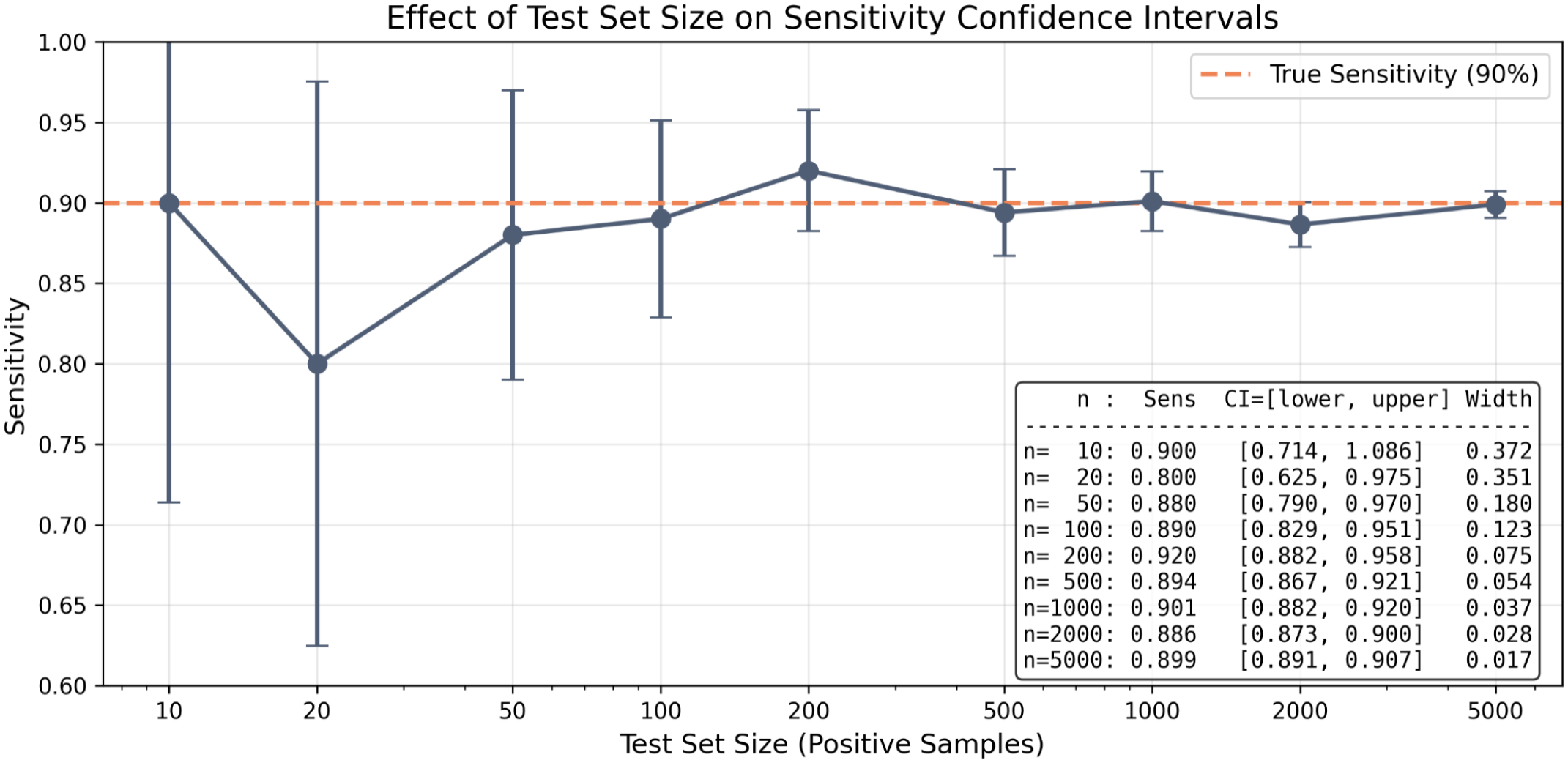
Relationship of the number of cases/images for an image classification task with its 95% confidence intervals. This simulation shows the high degree of uncertainty in the point estimate of the performance metric sensitivity when the test data set consists of too few cases. The simulation was conducted using a binomial sampling model assuming a true underlying sensitivity of 90%. For each test set size, the number of true positives was drawn from a binomial distribution (n trials, P = .90), and sensitivity was calculated as the proportion of correctly identified positive cases. This was repeated across test set sizes ranging from 10 to 5000 positive samples. Confidence intervals (95%) were computed using the normal approximation method (z = 1.96), with interval width calculated as $\pm 1.96 \sqrt{p (1 - p) / n} .$ Error bars in the figure represent these 95% confidence intervals.

When the default 3-way data set split results in a small, nonrepresentative test subset, the k-fold cross-validation approach may be used as an alternative. In this method, the data set is divided at the patient level into several (number indicated by k) subsets (folds), and each fold is used independently for training, validation, or testing across multiple iterations of model development.⁵¹ This approach enables that every image in the data set is used for testing in at least one fold, thereby increasing the variability of images tested across all folds combined. However, due to the increased computational resources required to develop multiple models, cross-validation is typically reserved for small data sets. Note that not all commercial software packages allow automation of the cross-validation process.

In addition to the sample size, test data sets must also be representative and cover a realistic variance of images. This means that the image features in the test set should reflect those of the real-world use case for which the model is intended.^27,33 For example, if a mitotic figure detection algorithm is intended to analyze entire WSIs, it must be tested on images from all regions of a WSI and not only perfect regions of interest (intraslide variability). At the same time, the use of a single WSI with thousands of annotations may be less informative than using multiple random regions of interest from numerous tumor cases, which better encompass the interslide variability. Another example is if the model is intended for use in different laboratories, it must be tested on samples prepared in various laboratories and digitized using different WSI scanners. To sufficiently encompass the intended use case, a large and diverse test data set may be required that encompasses a realistic variability in tissue quality, tissue morphology (eg, different disease subtypes), slide preparation and digitization methods (eg, staining, ink, and color representation), and artifacts (eg, tissue folds and scan artifacts). In some cases, oversampling of certain case subgroups (as compared with their actual frequency) may be favorable to include all relevant morphological subtypes and allow for stratified performance evaluation of relevant variables.⁴⁰ In contrast, active-learning based image selection and synthetic images should not be used for test data sets, since they do not ensure a realistic and real-world image representation.¹³ This discussion in test set representativeness also implies that any change in the laboratory workflow (eg, a new WSI scanner or a change of the staining process) may make this new application case out-of-domain, which may necessitates extension of the test set and reevaluation of model performance.

Previous analysis of AI articles has highlighted the importance of test set size and variability, showing that removing a single case from a small test set can significantly alter performance metrics.⁴² Statistical methods that calculate confidence intervals for performance metrics may help mitigate this effect and provide uncertainty estimates for the point estimate. The analytical derivation of confidence intervals can be challenging, particularly for complex metrics or structured data. Therefore, resampling methods such as bootstrapping are highly attractive, as they can be applied to a broad range of metrics with relatively few assumptions. In a case-level stratified bootstrap, predictions on the test data set are repeatedly resampled with replacements at the level of independent units, and the metric of interest is recalculated for each resample. The empirical distribution of these bootstrapped metric values can then be used to derive confidence intervals.²² Resampling approaches are also useful when comparing different DL models or training strategies on the same test set. In such paired settings, bootstrap methods can estimate the distribution of the difference between 2 models’ performance metrics across resamples, allowing the calculation of confidence intervals for these differences. This enables an assessment of whether an observed performance improvement is likely to be meaningful or falls within the range of random variation due to the finite and possibly heterogeneous test data set.

The quality of the ground truth is a critical consideration for test data sets.²⁸ Errors in the ground-truth labels of the test set (such as oversegmentation or undersegmentation, omission or addition of an object) have been shown to significantly bias the determined performance metrics.²⁸ As discussed above, ground-truth annotations by pathologists are inherently subject to bias, and errors in the ground truth of the test set can unjustly diminish algorithmic performance. A well-planned annotation workflow (including detailed annotation instructions with clear definitions of the label classes) and, depending on the complexity of the pattern of interest, advanced annotation methods may be necessary to reduce annotation biases.¹³ These methods may include majority voting by multiple annotators,⁶⁸ computer-assisted identification of missed candidates,¹² or decisions guided by providing additional staining through image registration.²⁵ On the contrary, algorithmically generated labels (to speed up the annotation process) may diminish label quality and careful review by experts is critical.⁴⁴

Finally, authors of articles on DL-AIA should consider making their test data sets (or entire data sets) publicly available. Open access to these data sets allows other researchers to evaluate their algorithms on external images, facilitating comparisons and providing a valuable resource for assessing algorithmic robustness.⁴⁰ However, systematic differences in the ground truth (label shift) between the in-house and external data set must be considered as potential sources for a drop in performance.¹² Considering the paucity of open data sets,¹³ a relevant limitation of current DL research is that only a few data sets are frequently used for the development of state-of-the-art DL methods.⁶³ While a continuous, slight improvement in performance may be reported in the literature over time, this may reflect hyperparameter overfitting to a specific data set rather than an actual improvement in the DL method. This consideration highlights the need for more researchers to make their data set accessible to facilitate performance evaluations of innovative DL-AIA methods.

Statistical Comparison of Deep Learning Models on the Same Test Data Set

In many DL-AIA studies, multiple model development methods are compared with identify the approach that yields the best performance, which is ideally supported by statistical comparisons. The differences in the model development may be related to different model architectures, alternative training strategies, or varied hyperparameters. These models are usually tested on the same hold-out test set. This means that for each animal, patient, or WSI in the test set, every model makes a prediction on exactly the same case. The results of 2 models are therefore not independent, they are paired case by case. This paired structure is important, because it allows more sensitive and appropriate statistical comparisons that directly examine whether the performance of 2 models is actually different. These considerations, and suitable statistical methods for exploiting such paired structures, are described in the following paragraphs.²¹

A first principle in such comparisons is to define the independent unit of analysis appropriately. In biomedical image analysis, this unit is often the patient, animal, or slide, and not necessarily the individual tile, or candidate detection, which may be nested within a higher-level unit. All inferential procedures and any resampling strategy should therefore respect the underlying clustering structure of the data.

If performance metrics are available at the level of individual independent cases, paired statistical methods are appropriate. For binary case-level outcomes, such as correct versus incorrect diagnosis per patient or slide, McNemar’s test is a widely used method for comparing 2 models on paired data.^21,45 McNemar’s test focuses on discordant pairs, that is, cases on which the 2 models disagree, and assesses whether one model is systematically more often correct than the other. For continuous or count-based case-level outcomes, such as per-slide mitotic counts, cell densities, or segmentation overlap scores, comparisons between 2 models can be performed using paired t-tests when distributional assumptions are reasonable, or Wilcoxon signed-rank tests when a less assumption-dependent alternative is preferred. More generally, permutation tests based on within-case differences provide a robust nonparametric alternative that preserves the paired design.

When several models are compared simultaneously, linear mixed models for approximately continuous case-level outcomes and generalized linear mixed models for binary case-level outcomes provide a flexible framework for analysis. In these models, model identity is treated as a fixed effect, whereas a case is included as a random effect, or equivalently as a repeated factor, to account for the fact that all models are evaluated on the same cases. This approach estimates average performance differences between model configurations while accounting for the fact that cases vary in their inherent difficulty.

For object detection tasks, performance can be summarized either as a pooled (microaveraged) metric, where performance across all objects in the data set is aggregated globally, or as a case/group-level metric, which is computed separately for each independent group, and afterwards group-level results are averaged (macroaveraging).^8,64 The choice between these approaches should be driven by the scientific or clinical question. A pooled metric gives greater weight to cases contributing many objects and reflects overall object-level detection performance. In contrast, a case-level summary gives equal weight to each independent unit and may better reflect clinically relevant variation across patients. For mitotic figure detection, a pooled F1-score is often reported because it summarizes object-level detection across all candidate mitotic figures. However, a case-level formulation may be preferable when the practical consequences of model errors depend on how those errors are distributed across slides or patients. If case-level metrics are considered most relevant, their paired structure naturally supports paired tests, permutation tests, or mixed-effects models.

If only a single pooled metric per model is of interest, such as one overall F1-score computed across the entire test set, the paired structure is no longer represented as one observation per case. In this situation, model comparison should rely on resampling or permutation procedures that preserve the paired evaluation of all models on the same test cases. A suitable approach is a paired or cluster bootstrap, in which the independent test units (eg, patients, slides, or images) are resampled with replacements, and the pooled metric is recomputed for each model within each bootstrap sample.²² Comparisons should then be based on the empirical distribution of paired performance differences, such as

Δ F 1 = F 1_{A} - F 1_{B}

from which confidence intervals and, if desired, P values can be obtained. Importantly, inference should be based on the confidence interval of the difference between models, rather than visual inspection of overlap between separate confidence intervals for each model. Overlap of two 95% confidence intervals is only a heuristic and may be misleading.^4,19 Because bootstrap replicates are resampled versions of the same test data set rather than independent observations, they should not be treated as independent response values in a mixed-effects model.

Regardless of whether case-level or pooled metrics are analyzed, hypothesis testing should be complemented by effect size estimates and confidence intervals for the difference in performance between models, such as differences in accuracy, F1-score, Dice coefficient, or area under the curve.⁶² These measures are often more informative than p-values alone because they describe both the magnitude and the uncertainty of any improvement. In bootstrap-based analyses, this is naturally achieved by examining the empirical distribution of paired performance differences across resamples. If the confidence interval for the difference excludes zero, this supports a statistically detectable difference between models. However, the practical importance of that difference should still be judged in light of the clinical or biological application.

A common pitfall in model comparisons arises when many models or configurations are tested on the same data set, leading to a multiple comparison problem. For example, if 20 different hyperparameter configurations are each compared with a baseline model using a significance threshold of P < .05, one would expect at least one “significant” result by chance alone, even if no true differences exist.⁶ This inflates the risk of falsely concluding that a particular model is superior. When multiple pairwise comparisons are conducted, appropriate corrections (eg, Bonferroni, Holm, or false discovery rate adjustments) should be applied, or the analysis should be reframed as an exploratory investigation rather than confirmatory hypothesis testing.^6,32 Alternatively, researchers may choose to prespecify a small number of key comparisons or rely primarily on effect sizes and confidence intervals, which are less prone to inflation from multiple testing and provide more interpretable evidence of practical differences.^62,67

An additional caveat applies when test data sets are very large or when performance is evaluated at the level of thousands of tiles or individual objects rather than independent cases. In such scenarios, even trivial differences in performance can yield highly significant P values, leading to overinterpretation of negligible improvements. For this reason, statistical comparison should always be anchored in clinical or biological relevance (eg, whether the observed difference in performance translates into meaningful change in diagnostic accuracy, workload reduction, or patient outcome). Visual inspection of error distributions, stratified analyses by case difficulty or image domain, and secondary performance indices, such as correlation with pathologist scores or discriminability of prognostic groups, can all help contextualize whether a statistically significant difference is also practically important.

Multiple Training Runs and Statistical Comparison of Model Stability

Due to the stochastic nature of DL model training (eg, random weight initialization, stochastic optimization, and random data augmentation), repeated training of the same architecture on the same data can yield slightly different models with different performance metrics. Consequently, a single training run may not adequately reflect the typical performance of a particular model configuration. To better characterize model stability and to avoid overinterpreting potentially optimistic or pessimistic single-run results, it is advisable to train each candidate model configuration multiple times with different random seeds and to summarize performance across these runs.^14,15

In many practical DL-AIA applications, however, computational constraints limit the number of independent runs to a relatively small number (eg, 3–5 per configuration). When only a single aggregate performance metric, such as F1-score or Dice coefficient over the entire test set, is available for each run, the resulting sample size for between-configuration comparisons is therefore very small, and the runs are not strictly independent because they are trained and evaluated on the same underlying data. While, in principle, paired statistical tests (such as a paired t-test or Wilcoxon signed-rank test) could be applied to the per-run metrics of 2 configurations, the small number of runs and the lack of true independence between runs limit the reliability and interpretability of such tests. In this context, repeated runs are best regarded primarily as a model stability and sensitivity analysis, demonstrating whether performance is broadly consistent across seeds, rather than as a basis for strong inferential claims about the superiority of one configuration over another. Large variability across runs suggests that the model is sensitive to random factors and may not be reliable in routine use, even if the best-performing run shows high metrics.¹⁵

More formal statistical comparison of model configurations benefits from having either a larger number of independent runs per configuration or the ability to resample the test data at the level of independent units (eg, animals, patients, and WSIs). In the latter case, bootstrap resampling of the test set can be combined with multiple training runs to account for both sources of variability: for each of K training runs, the test set is resampled with replacements B times (eg, B = 1000) at the case level, and the aggregate performance metric is recalculated for each bootstrap sample. This yields a distribution of performance metrics that reflects both training stochasticity (across runs) and sampling variability (across bootstrap resamples). Confidence intervals for performance metrics and for differences between configurations (Δmetrics) can then be derived from these combined distributions, providing a more nuanced and reliable assessment than single p-values.^21,22 When sufficient K × B samples are available, formal comparisons can be based on the empirical distribution of Δmetrics (eg, bootstrap confidence intervals or nonparametric paired tests), but interpretation should still focus on effect sizes and confidence intervals rather than p-values, particularly when many model configurations or hyperparameter settings are explored in parallel.^62,67 In all scenarios, emphasis should be placed on the magnitude and clinical relevance of observed differences, with repeated runs serving to demonstrate that reported performance is stable rather than the result of a single favorable training outcome.

Conclusion

In conclusion, proper performance evaluation of DL-AIA algorithms is essential before their implementation into research or diagnostic workflows to ensure their safe and effective use. Numerous challenges exist, particularly because these models are typically (with few exceptions) compared with pathologists’ decisions and therefore inherit all limitations of an imperfect reference standard, including interobserver and intraobserver variabilities and ambiguities in diagnostic thresholds. This comparison can be conducted either through visual assessment or by calculating the differences between predictions and ground-truth annotations (statistical evaluation), and both approaches are currently used in veterinary DL-AIA publications.

This article highlights that exclusive reliance on visual assessment is not sufficient for evaluating complex DL models and has substantial limitations in terms of transparency, reproducibility, and the ability to communicate performance in a manner that is comparable across studies. Statistical evaluation, although more time-intensive due to the need for high-quality ground-truth annotations and carefully designed test data sets, enables the use of clearly defined performance metrics, confidence intervals, and benchmarks, and facilitates rigorous comparisons of different models and training strategies. At the same time, visual assessment remains indispensable for understanding the morphology of false predictions, identifying systematic failure modes, and guiding data set refinement. In practice, visual and statistical evaluations provide complementary information, and a combination of both yields the most comprehensive understanding of the overall performance and specific sources of error.

Reliable statistical performance evaluation requires more than just reporting a single metric on a convenient test set. It critically depends on the availability of an independent and representative (“real-world”) test data set, created with appropriate data splitting to avoid leakage, and with sufficient size and variability to capture the intended use case. Sample size considerations at the case level, together with confidence intervals and resampling methods such as bootstrapping, help to avoid overinterpretation of unstable point estimates, particularly in small or unbalanced test sets. Furthermore, thoughtful metric selection tailored to the pathology task, along with the use of multiple complementary metrics, is necessary to ensure that the reported performance truly reflects the clinically relevant aspects of the algorithm’s behavior. Thus, evaluating the model on multiple levels (eg, pattern recognition task, pathology task, and measurement level) may be needed. When multiple models or configurations are compared, paired analyses, resampling-based confidence intervals for metric differences, and careful handling of multiple comparisons are essential to distinguish meaningful improvements from random variation or overfitting to a specific data set. Finally, given the stochastic nature of DL training, repeated runs with different random seeds are crucial to assess model stability. When feasible, combining these multiple runs with case-level resampling quantifies uncertainty from both training stochasticity and finite test sample size.

By outlining these considerations and summarizing them in Supplemental Table S1, we aim to support the development of good scientific practice in veterinary DL-AIA and to lay the groundwork for ongoing discussion within the veterinary pathology community on best practices for evaluating DL models.

Supplemental Material

sj-xlsx-1-vet-10.1177_03009858261461760 – Supplemental material for Performance evaluation of deep learning models for image analysis: Considerations for visual assessment and statistical metrics

Supplemental material, sj-xlsx-1-vet-10.1177_03009858261461760 for Performance evaluation of deep learning models for image analysis: Considerations for visual assessment and statistical metrics by Christof A. Bertram, Jonas Ammeling, Alexander Bartel, Gillian Beamer and Marc Aubreville in Veterinary Pathology

Supplemental Material

sj-pdf-1-vet-10.1177_03009858261461760 – Supplemental material for Performance evaluation of deep learning models for image analysis: Considerations for visual assessment and statistical metrics

Supplemental material, sj-pdf-1-vet-10.1177_03009858261461760 for Performance evaluation of deep learning models for image analysis: Considerations for visual assessment and statistical metrics by Christof A. Bertram, Jonas Ammeling, Alexander Bartel, Gillian Beamer and Marc Aubreville in Veterinary Pathology

Footnotes

Acknowledgements

The author(s) acknowledge the use of ChatGPT (OpenAI and GPT-4) for assistance with proofreading and improving the clarity of the manuscript. The author(s) take full responsibility for the content, accuracy, and interpretation of the work presented in this publication.

Supplemental material for this article is available online.

Author’s Contributions

CAB, JA, and MA conceived the manuscript; all authors contributed to content discussions. The manuscript was written by CB and JA with contribution from the other authors.

Declaration of Conflicting Interests

The authors declared the following potential conflicts of interest with respect to the research, authorship, and/or publication of this article: Authors Christof Bertram and Marc Aubreville are members of the Editorial Board of Veterinary Pathology and have no further conflicts to declare.

Funding

The authors disclosed receipt of the following financial support for the research, authorship, and/or publication of this article: CAB acknowledges support from the Austrian Research Fund (FWF, project number: I 6555). JA acknowledges support by the Bavarian State Ministry for Science and the Arts (project FOKUS-TML). MA acknowledges support by the Deutsche Forschungsgemeinschaft (DFG, project number: 520330054).

ORCID iDs

Christof A. Bertram

Jonas Ammeling

Alexander Bartel

Marc Aubreville

References

Aeffner

Wilson

Martin

, et al. The gold standard paradox in digital image analysis: manual versus automated scoring as ground truth. Arch Pathol Lab Med. 2017;141:1267–1275. doi:10.5858/arpa.2016-0386-RA.

Aubreville

Stathonikos

Bertram

, et al. Mitosis domain generalization in histopathology images–the MIDOG challenge. Med Image Anal. 2023;84:102699. doi:10.1016/j.media.2022.102699.

Aubreville

Stathonikos

Donovan

, et al. Domain generalization across tumor types, laboratories, and species–Insights from the 2022 edition of the mitosis domain generalization challenge. Med Image Anal. 2024;94:103155. doi:10.1016/j.media.2024.103155.

Austin

Hux

JE.

A brief note on overlapping confidence intervals. J Vasc Surg. 2002;36:194–195. doi:10.1067/mva.2002.125015.

Bédard

Westerling-Bui

Zuraw

Proof of concept for a deep learning algorithm for identification and quantification of key microscopic features in the murine model of DSS-induced colitis. Toxicol Pathol. 2021;49:897–904. doi:10.1177/0192623320987804.

Benjamini

Hochberg

Controlling the false discovery rate: a practical and powerful approach to multiple testing. J Royal Stat Soc: Series B (Methodological). 1995;57:289–300.

Bertani

Blanck

Guignard

, et al. Artificial intelligence in toxicological pathology: quantitative evaluation of compound-induced follicular cell hypertrophy in rat thyroid gland using deep learning models. Toxicol Pathol. 2022;50:23–34. doi:10.1177/01926233211052010.

Bertram

Aubreville

Donovan

, et al. Computer-assisted mitotic count using a deep learning-based algorithm improves interobserver reproducibility and accuracy. Vet Pathol. 2022;59:211–226. doi:10.1177/03009858211067478.

Bertram

Donovan

Tecilla

, et al. Dataset on bi-and multi-nucleated tumor cells in canine cutaneous mast cell tumors. In: Palm

Deserno

Handels

Maier

Maier-Hein

Tolxdorff

, eds. Bildverarbeitung für die Medizin 2021. New York: Springer Vieweg; 2021:134–139.

10.

Bertram

Marzahl

Bartel

, et al. Cytologic scoring of equine exercise-induced pulmonary hemorrhage: performance of human experts and a deep learning-based algorithm. Vet Pathol. 2023;60:75–85. doi:10.1177/03009858221137582.

11.

Bertram

Schutten

Ressel

, et al. Reporting guidelines for manuscripts that use artificial intelligence-based automated image analysis in veterinary pathology. Vet Pathol. 2025;62:615–617. doi:10.1177/03009858251344320.

12.

Bertram

Veta

Marzahl

, et al. Are pathologist-defined labels reproducible? Comparison of the TUPAC16 mitotic figure dataset with an alternative set of labels. In: Cardoso

Feragen

Glocker

, et al, eds. Interpretable and Annotation-Efficient Learning for Medical Image Computing. Lecture Notes in Computer Science. Vol. 12446. Springer; 2020:204–213.

13.

Bertram

Weiss

Ammeling

, et al. Dataset creation for supervised deep learning-based analysis of microscopic images-review of important considerations and recommendations. arXiv preprint. 2512.04564; 2025.

14.

Bouthillier

Delaunay

Bronzi

, et al. Accounting for variance in machine learning benchmarks. Proceed Mach Learn Syst. 2021;3:747–769.

15.

Bouthillier

Laurent

Vincent

Unreproducible research is reproducible. Proceedings of the International Conference on Machine Learning (ICML); June 2019; Long Beach, CA.

16.

Bussola

Marcolini

Maggio

, et al. AI slipping on tiles: data leakage in digital pathology. In: Del Bimbo

Cucchiara

Sclaroff

, et al., eds. Pattern Recognition. ICPR International Workshops and Challenges. ICPR 2021. Lecture Notes in Computer Science. Vol. 12661. Cham: Springer; 2021: 167–182.

17.

Carboni

Marxfeld

Tuoken

, et al. A workflow for the performance of the differential ovarian follicle count using deep neuronal networks. Toxicol Pathol. 2021;49:843–850. doi:10.1177/0192623320969130.

18.

Creasy

Panchal

Garg

, et al. Deep learning-based spermatogenic staging assessment for hematoxylin and eosin-stained sections of rat testes. Toxicol Pathol. 2021;49:872–887. doi:10.1177/0192623320969678.

19.

Cumming

Inference by eye: reading the overlap of independent confidence intervals. Stat Med. 2009;28:205–220. doi:10.1002/sim.3471.

20.

De Vera Mudry

Martin

Schumacher

, et al. Deep learning in toxicologic pathology: a new approach to evaluate rodent retinal atrophy. Toxicol Pathol. 2021;49:851–861. doi:10.1177/0192623320980674.

21.

Dietterich

TG.

Approximate statistical tests for comparing supervised classification learning algorithms. Neural Comput. 1998;10:1895–1923. doi:10.1162/089976698300017197.

22.

Efron

Tibshirani

RJ.

An introduction to the bootstrap. Chapman and Hall/CRC; 1994

23.

Fragoso -Garcia

Wilm

Bertram

, et al. Automated diagnosis of 7 canine skin tumors using machine learning on H&E-stained whole slide images. Vet Pathol. 2023;60:865–875. doi:10.1177/03009858231189205.

24.

Funk

Clement

Togninalli

, et al. Comparison of an attention-based Multiple Instance Learning (MIL) with a visual transformer model: two weakly supervised Deep Learning (DL) algorithms for the detection of histopathologic lesions in the rat liver to distinguish normal from abnormal. Toxicol Pathol. 2025;53:456–478. doi:10.1177/01926233251339653.

25.

Ganz

Marzahl

Ammeling

, et al. Information mismatch in PHH3-assisted mitosis annotation leads to interpretation shifts in H&E slide analysis. Sci Rep. 2024;14:26273. doi:10.1038/s41598-024-77244-6.

26.

Haghofer

Parlak

Bartel

, et al. Nuclear pleomorphism in canine cutaneous mast cell tumors: comparison of reproducibility and prognostic relevance between estimates, manual morphometry, and algorithmic morphometry. Vet Pathol. 2025;62:161–177. doi:10.1177/03009858241295399.

27.

Hanna

Olson

Zarella

, et al. Recommendations for performance evaluation of machine learning in pathology: a concept paper from the College of American Pathologists. Arch Pathol Lab Med. 2024;148:e335–e361. doi:10.5858/arpa.2023-0042-CP.

28.

Harada

Nomura

Komura

, et al. Label noise in pathological segmentation is overlooked, leading to potential overestimation of artificial intelligence. Cancer Sci. 2026;117:852–863. doi:10.1111/cas.70288.

29.

Heinemann

Lempp

Colbatzky

, et al. Quantification of hepatocellular mitoses in a toxicological study in rats using a convolutional neural network. Toxicol Pathol. 2022;50:344–352. doi:10.1177/01926233221083500.

30.

Hill

Koback

Schilling

PL.

The risk of shortcutting in deep learning algorithms for medical imaging research. Sci Rep. 2024;14:29224. doi:10.1038/s41598-024-79838-6.

31.

Hoefling

Sing

Hossain

, et al. HistoNet: a deep learning-based model of normal histology. Toxicol Pathol. 2021;49:784–797. doi:10.1177/0192623321993425.

32.

Holm

A simple sequentially rejective multiple test procedure. Scandinav J Stat. 1979;6:65–70.

33.

Homeyer

Geißler

Schwen

, et al. Recommendations on compiling test datasets for evaluating artificial intelligence solutions in pathology. Mod Pathol. 2022;35:1759–1769. doi:10.1038/s41379-022-01147-y.

34.

Schutt

Kozlowski

, et al. Ovarian toxicity assessment in histopathological images using deep learning. Toxicol Pathol. 2020;48:350–361. doi:10.1177/0192623319877871.

35.

Hüllermeier

Waegeman

Aleatoric and epistemic uncertainty in machine learning: an introduction to concepts and methods. Mach Learn. 2021;110:457–506.

36.

Hvid

Skydsgaard

Jensen

, et al. Artificial intelligence-based quantification of epithelial proliferation in mammary glands of rats and oviducts of göttingen minipigs. Toxicol Pathol. 2021;49:912–927. doi:10.1177/0192623320950633.

37.

Hwang

Kim

Park

, et al. Implementation and practice of deep learning-based instance segmentation algorithm for quantification of hepatic fibrosis at whole slide level in sprague-dawley rats. Toxicol Pathol. 2022;50:186–196. doi:10.1177/01926233211057128.

38.

Inai

Izawa

Kamei

, et al. Difference in the mechanism of iron overload-enhanced acute hepatotoxicity induced by thioacetamide and carbon tetrachloride in rats. Toxicol Pathol. 2024;52:55–66. doi:10.1177/01926233241235623.

39.

Janowczyk

Madabhushi

Deep learning for digital pathology image analysis: a comprehensive tutorial with selected use cases. J Pathol Inform. 2016;7:29. doi:10.4103/2153-3539.186902.

40.

Javed

Juyal

Shanis

, et al. Rethinking machine learning model evaluation in pathology. arXiv preprint. 2204.05205; 2022.

41.

Kuklyte

Fitzgerald

Nelissen

, et al. Evaluation of the use of single- and multi-magnification convolutional neural networks for the determination and quantitation of lesions in nonclinical pathology studies. Toxicol Pathol. 2021;49:815–842. doi:10.1177/0192623320986423.

42.

Maier-Hein

Eisenmann

Reinke

, et al. Why rankings of biomedical image analysis competitions should be interpreted with care. Nat Commun. 2018;9:5217. doi:10.1038/s41467-018-07619-7.

43.

Maier-Hein

Reinke

Godau

, et al. Metrics reloaded: recommendations for image analysis validation. Nat Methods. 2024;21:195–212. doi:10.1038/s41592-023-02151-z.

44.

Marzahl

Bertram

Aubreville

, et al. Are fast labeling methods reliable? A case study of computer-aided expert annotations on microscopy slides. In: Martel

Abolmaesumi

Stoyanov

, et al., eds. Medical Image Computing and Computer Assisted Intervention—MICCAI 2020. Lecture Notes in Computer Science. Vol 12261. Cham: Springer; 2020: 24–32.

45.

McNemar

Note on the sampling error of the difference between correlated proportions or percentages. Psychometrika. 1947;12:153–157. doi:10.1007/BF02295996.

46.

Mecklenburg

Luetjens

Romeike

, et al. Deep learning-based spermatogenic staging in tissue sections of cynomolgus macaque testes. Toxicol Pathol. 2024;52:4–12. doi:10.1177/01926233241234059.

47.

Mehrvar

Kambara

Morphologic features and deep learning-based analysis of canine spermatogenic stages. Toxicol Pathol. 2022;50:736–753. doi:10.1177/01926233221117747.

48.

Mehrvar

Maisonave

Buck

, et al. Immunohistochemistry-free enhanced histopathology of the rat spleen using deep learning. Toxicol Pathol. 2025;53:83–94. doi:10.1177/01926233241303907.

49.

Meuten

Moore

Donovan

, et al. International guidelines for veterinary tumor pathology: A call to action. Vet Pathol. 2021;58:766–794. doi:10.1177/03009858211013712.

50.

Naylor

McInnes

Alibhai

, et al. Development of a deep learning tool to support the assessment of thyroid follicular cell hypertrophy in the rat. Toxicol Pathol. 2025;53:240–250. doi:10.1177/01926233241309328.

51.

Pacholec

Flatland

Xie

, et al. Harnessing artificial intelligence for enhanced veterinary diagnostics: a look to quality assurance, Part I Model development. Vet Clin Pathol. 2024;54:S30–S42. doi:10.1111/vcp.13401.

52.

Palazzi

Barale -Thomas

Bawa

, et al. Results of the European society of toxicologic pathology survey on the use of artificial intelligence in toxicologic pathology. Toxicol Pathol. 2023;51:216–224. doi:10.1177/01926233231182115.

53.

Pischon

Mason

Lawrenz

, et al. Artificial intelligence in toxicologic pathology: quantitative evaluation of compound-induced hepatocellular hypertrophy in rats. Toxicol Pathol. 2021;49:928–937. doi:10.1177/0192623320983244.

54.

Puget

Ganz

Ostermaier

, et al. Artificial intelligence can be trained to predict c-KIT-11 mutational status of canine mast cell tumors from hematoxylin and eosin-stained histological slides. Vet Pathol. 2025;62:152–160. doi:10.1177/03009858241286806.

55.

Ramot

Deshpande

Morello

, et al. Microscope-based automated quantification of liver fibrosis in mice using a deep learning algorithm. Toxicol Pathol. 2021;49:1126–1133. doi:10.1177/01926233211003866.

56.

Ramot

Zandani

Madar

, et al. Utilization of a deep learning algorithm for microscope-based fatty vacuole quantification in a fatty liver model in mice. Toxicol Pathol. 2020;48:702–707. doi:10.1177/0192623320926478.

57.

Rosbach

Ammeling

Ganz

, et al. Stuck on suggestions: automation bias, the anchoring effect, and the factors that shape them in computational pathology. MELBA–BVM 2025 Special Issue. 2026;2026:126–147. doi:10.59275/j.melba.2026-87b1.

58.

Rosbach

Ammeling

Krügel

, et al. “When two wrongs don’t make a right”-Examining confirmation bias and the role of time pressure during human-AI collaboration in computational pathology. Proceedings of the 2025 CHI Conference on Human Factors in Computing Systems; April 2025; Yokohama, Japan.

59.

Rudmann

Albretsen

Doolan

, et al. Using deep learning artificial intelligence algorithms to verify N-Nitroso-N-Methylurea and urethane positive control proliferative changes in Tg-RasH2 mouse carcinogenicity studies. Toxicol Pathol. 2021;49:938–949. doi:10.1177/0192623320973986.

60.

Smith

Westerling -Bui

Wilcox

, et al. Screening for bone marrow cellularity changes in cynomolgus macaques in toxicology safety studies using artificial intelligence models. Toxicol Pathol. 2021;49:905–911. doi:10.1177/0192623320981560.

61.

Stacke

Eilertsen

Unger

, et al. Measuring domain shift for deep learning in histopathology. IEEE J Biomed Health Inform. 2021;25:325–336. doi:10.1109/jbhi.2020.3032060.

62.

Sullivan

Feinn

Using effect size-or why the P value is not enough. J Grad Med Educ. 2012;4:279–282. doi:10.4300/jgme-d-12-00156.1.

63.

Tafavvoghi

Bongo

Shvetsov

, et al. Publicly available datasets of breast histopathology H&E whole-slide images: a scoping review. J Pathol Inform. 2024;15:100363. doi:10.1016/j.jpi.2024.100363.

64.

Takahashi

Yamamoto

Kuchiba

, et al. Confidence interval for micro-averaged F (1) and macro-averaged F (1) scores. Appl Intell (Dordr). 2022;52:4961–4972. doi:10.1007/s10489-021-02635-5.

65.

Tokarz

Steinbach

Lokhande

, et al. Using artificial intelligence to detect, classify, and objectively score severity of rodent cardiomyopathy. Toxicol Pathol. 2021;49:888–896. doi:10.1177/0192623320972614.

66.

Vuorimaa

Kareinen

Toivanen

, et al. Deep learning-based segmentation of morphologically distinct rat hippocampal reactive astrocytes after trimethyltin exposure. Toxicol Pathol. 2022;50:754–762. doi:10.1177/01926233221124497.

67.

Wasserstein

Schirm

Lazar

NA.

Moving to a world beyond “p< 0.05.”

Am Statistic. 2019;73(suppl 1):1–19.

68.

Wilm

Bertram

Marzahl

, et al. Influence of inter-annotator variability on automatic mitotic figure assessment. In: Palm

Deserno

Handels

, et al., eds. Bildverarbeitung Für Die Medizin 2021. Informatik Aktuell. Wiesbaden: Springer Vieweg; 2021: 241–246.

69.

Wulcan

Giaretta

Fingerhood

, et al. Artificial intelligence-based quantification of lymphocytes in feline small intestinal biopsies. Vet Pathol. 2025;62:139–151. doi:10.1177/03009858241286828.

70.

Xie

Thibault

Shirai

, et al. Deep learning methodology for quantification of normal pancreas structures. Toxicol Pathol. 2025;53:554–560. doi:10.1177/01926233251341824.

Supplementary Material

Please find the following supplemental material available below.

For Open Access articles published under a Creative Commons License, all supplemental material carries the same license as the article it is associated with.

For non-Open Access articles published, all supplemental material carries a non-exclusive license, and permission requests for re-use of supplemental material or any part of supplemental material shall be sent directly to the copyright owner as specified in the copyright notice associated with the article.

0.02 MB

0.38 MB