Prediction of slab surface longitudinal crack based on resampling and the Bayesian optimisation of LightGBM

Abstract

Longitudinal crack is a typical surface defect for slab of steel. Accurate prediction of longitudinal crack is of great significance to improve slab quality. However, in actual production, the quantity distribution of normal and longitudinally cracked slabs is extremely unbalanced, which brings great challenges to the subsequent modeling and prediction. To solve the above problems, this paper proposes a prediction method for the longitudinal crack under the condition of data imbalance. Firstly, multiple sampling methods (SMOTE, BorderlineSMOTE, SMOTE-ENN and SMOTE-Tomk) were used to construct feature data sets respectively to alleviate the problem of data imbalance. Then, based on the data sets after sampling processing, the prediction models of the longitudinal crack were constructed by using Random Forest (RF), Support Vector Machine (SVM), Logistic Regression (LR), XGBoost and LightGBM as classification algorithms. The models’ hyperparameters were determined by Bayesian optimisation and the optimal classification algorithm was selected according to the evaluation metrics. Meantime, SHapley Additive exPlanations (SHAP) was used to analyse the model and verify the influence of input parameters on the model output. The results show that, compared with other models, the combined model of SMOTE sampling and LightGBM classification algorithm can better deal with the problem of imbalanced data for prediction of the longitudinal crack. The Recall of normal and longitudinally cracked slabs are 90.57% and 84.62%, respectively, false alarm rate is 9.44% and AUC is 0.93. At the same time, the training time of this model is about 0.15 s, and prediction time is less than 0.01 s. The time consumed in each stage is significantly shorter than other models. It shows obvious advantages and provides a reliable method for predicting the longitudinal crack.

Keywords

Continuous casting slab surface longitudinal crack resampling lightGBM SHAP Bayesian optimisation

Introduction

High-efficiency continuous casting with defect-free slab as the core content is not only the basis for hot charging and direct rolling, but also an important goal and direction for the development of modern continuous casting technology.¹ How to achieve defect-free slab production has always been a hot and difficult topic in the steel industry. With the development of new generation information technologies such as big data and artificial intelligence,^2,3 data-driven methods such as machine learning can efficiently mine the correlation between continuous casting process parameters and slab defects, and integrate process knowledge to establish a high-precision and fast-response slab defect prediction model, forming a positive interaction between the prediction model results and the actual continuous casting production. Therefore, it is expected to solve the problem of slab quality control in the continuous casting process and provide theoretical and technical support for defect-free slab production.

Longitudinal crack is one of the main defects affecting the quality of slabs, which is generally formed near the meniscus and further expanded under the cooling effect of the mould and secondary cooling section. In severe cases, it may cause scrap or breakout accidents, resulting in significant economic losses. So far, the research on the prediction methods of longitudinal crack on the surface of the slab by scholars at home and abroad can be attributed to mechanism models and data-driven models.

For mechanism models, it is common to construct a heat transfer/stress calculation model that describes the mould and solidified shell, coupled with the solution of the stress field distribution of the shell, and compare it with its physical and mechanical properties to establish a critical criterion for the crack, and then predict the formation of the longitudinal crack. Poltarak et al.⁴ established a thermal/mechanical coupling finite element model for round billet continuous casting to calculate the stress acting on the solidification front to assess the risk of cracks under different continuous casting parameters. Du et al.⁵ established a full-size finite element model of the slab and mould, and the simulation results showed that the crack sensitivity was the highest at 60–100 mm from the meniscus, which was consistent with the actual situation on site. Wang et al.⁶ established a two-dimensional unsteady heat transfer and solidification model based on the meshless Galerkin method, which has good accuracy and adaptability, and can predict the crack-sensitive area more effectively than the traditional finite element method. The mechanism model for predicting longitudinal cracks requires accurate stress/strain distribution obtained through simulation or theoretical calculation, which cannot adapt to the requirements of actual production conditions changes and unstable operation. Therefore, this kind of model is rarely used in practice, and more is to calculate and analyse the influence factors and action rules of the longitudinal crack off-line to guide the actual process optimisation.

For data-driven models, they can be divided into two categories depending on the source of their data: longitudinal crack prediction models driven by data of the thermocouple temperature on mould copper plate, and longitudinal crack prediction models driven by data of the main influencing factors. For the former, both domestically and internationally, it mainly focuses on the abnormal temperature change characteristics of the copper plate during the formation and propagation of the longitudinal crack in the mould. With the help of certain logical judgment algorithms or intelligent algorithms, longitudinal crack prediction is achieved by identifying these characteristics. Liu et al.⁷ proposed a visual detection method of slab surface longitudinal crack based on temperature difference thermography and computer image processing algorithm. They used the thermocouple temperature of mould copper plate to construct the thermography and extract the temperature change characteristics, geometric features, location features and propagation speed of the longitudinal crack. These characteristics can be used to judge longitudinal crack. Duan et al.⁸ combined SVM with the Principal Component Analysis (PCA) to develop a model for predicting longitudinal crack defects. PCA was used to reduce the dimension of multiple characteristics of longitudinal cracks, and SVM was used for classifying the principal components of temperature characteristics with different casting conditions. Zhang et al.⁹ used random forest to reduce the dimension of temperature characteristics in the process of longitudinal crack formation, screened out relevant features closely related to longitudinal cracks, and established a longitudinal crack detection model based on K-means clustering, which can correctly distinguish and identify longitudinal cracks and normal working condition samples. These models show high accuracy in predicting the longitudinal cracks with obvious abnormal temperature change characteristics from the thermocouples. However, due to the limited number of thermocouples arranged in the mould, many longitudinal cracks do not cause abnormal temperature changes from the thermocouples in actual production. For example, some longitudinal cracks may occur between two columns of thermocouples, and so on. Therefore, it is inevitable to affect the practical application effect of this kind of model.

About the studies on the longitudinal crack prediction models driven by data of the main influencing factors, there are numerous factors affecting the surface longitudinal cracks of slabs, and there is a non-linear relationship between these factors, making it difficult to describe them accurately with statistical models. Machine learning algorithms can effectively handle non-linearity, uncertainty and complexity, and they possess strong adaptability, self-learning capabilities, fault tolerance and robustness. Peng et al.¹⁰ established three different input feature-based principal component analysis support vector machine models, among which the model containing parameters related to heat transfer in the mould had the best prediction performance, with a prediction accuracy of 56.5% for defect samples, an improvement of 4.1% relative to the previous results, indicating a certain correlation between longitudinal cracks and comprehensive heat transfer in the mould. Sala et al.¹¹ proposed a hybrid input FCN-CNN-SE model that integrates static influencing factor data and multivariate dynamic thermocouple time series data into the model simultaneously. Compared with a single thermocouple signal prediction model, this model performs better. However, the highly imbalanced data category of longitudinally cracked slabs leads to biased prediction results. The prediction accuracy of this model for longitudinally cracked slabs is 33%, which needs to be improved. The prediction of longitudinal cracks on the surface of slabs is actually an extremely imbalanced binary classification problem with multidimensional features, which is difficult to handle. Currently, only a few researchers have conducted improvement studies on this problem. Wu et al.¹² proposed a multi-scale convolutional recurrent neural network model that uses random sampling to establish balanced datasets based on different sampling ratios. The experimental results showed that when the sampling ratio is 1:2, it can detect more longitudinally cracked slabs while ensuring the accuracy of normal slab predictions. Although the above scholars have solved the problem of class imbalance to some extent through ensemble algorithm ideas or random sampling methods, improving the prediction accuracy of longitudinally cracked slabs, there are many sampling methods for handling imbalanced data. Only a single sampling method has been studied, and the combination of different sampling methods and classification algorithms is not studied. At the same time, there are still shortcomings in the interpretability of prediction models.

In order to solve the issue of extreme imbalance in longitudinal crack samples, this paper uses SMOTE, BorderlineSMOTE, SMOTE-ENN and SMOTE-Tomek sampling algorithms to expand the training set to deal with the problem of data category imbalance. Based on the training set processed by multiple sampling algorithms, the SVM, LR, RF, XGBoost and LightGBM classification algorithms are used to establish the prediction models of the longitudinal crack. Bayesian optimisation algorithm is then used to search for the optimal hyperparameters for each model. The prediction performance of different models is compared based on evaluation metrics, and the optimal model for predicting the longitudinal crack is selected. Additionally, SHAP is used to interpret and analyse the model's prediction results to improve the interpretability of the model's predictions.

Relevant methods

Resampling

The presence of one or more classes as the dominant class and another class as the minority class in a dataset is a common problem in classification, namely data classification imbalance. Resampling is a method to address the uneven distribution of samples from the data level for imbalanced classification problems. The imbalanced data processing method based on resampling technology does not require changes to the model or algorithm, and has the characteristics of simple implementation and strong adaptability. According to different sampling strategies, resampling methods are mainly divided into three methods: undersampling, oversampling and mixed sampling.

The undersampling method achieves the purpose of balancing the samples of each class by reducing the number of samples in the majority class. However, deleting a large number of samples in the majority class will result in the loss of a large amount of information in the original data, ultimately affecting the accuracy of the classification algorithm. Common undersampling methods include random undersampling, Tomek Links and ENN (Edited Nearest Neighbours).^13–15 Random undersampling achieves the purpose of balancing classes by randomly selecting the same number of samples from the majority class as the minority class. This method is simple to operate, but randomly discarding samples from the majority class can cause the loss of key information in the data. ENN starts from the perspective of data distribution, first calculates the K nearest neighbours of each sample, and for samples in the majority class, if most or all of their nearest neighbours do not belong to their class, they are deleted. Tomeklinks is a rule-based enhancement of nearest neighbours, taking two samples belonging to different classes and having similar neighbours as a Tomek link pair. All samples belonging to the majority class in the Tomek Link pairs are removed, making the boundary between the two classes more obvious and facilitating subsequent modelling.

The oversampling method aim to balance datasets by interpolating or replicating minority class samples. SMOTE (Synthetic Minority Over-Sampling Technique) calculates the Euclidean distance between samples and randomly selects similar neighbouring samples to interpolate and synthesise new minority class samples. SMOTE¹⁶ can effectively alleviate the overfitting problem caused by oversampling, but when it generates new samples for minority class points on the boundary, the new points will also be on the class boundary, leading to a blurred classification boundary. To address the boundary blurring issue of SMOTE, Han et al.¹⁷ proposed Borderline-SMOTE, an improved SMOTE algorithm based on the boundary. It only oversamples samples between the boundaries of the majority and minority classes, unlike the existing oversampling method, which oversample all minority class samples or random subsets of the minority class.

Mixed sampling refers to the combination of different sampling methods, integrating oversampling and undersampling methods to handle imbalanced datasets, increasing the number of minority class samples while reducing the number of majority class samples. After the dataset processed by two or more resampling methods is fed into the model, the probability of overfitting and underfitting of the model is relatively reduced. Common mixed sampling methods include SMOTE-Tomek and SMOTE-ENN. The SMOTE-Tomek method combines SMOTE and Tomek links methods, using SMOTE to increase the data of minority samples and then further filtering with Tomek links method. Although mixed sampling is a good choice, how to accurately set the sampling number remains an unresolved issue.

LightGBM

LightGBM¹⁸ is an improved algorithm based on Gradient Boosting Decision Tree (GBDT). Its working principle is similar to GBDT. Using classification regression trees as the foundation, it approximates the residual value of the current decision tree using the negative gradient of the loss function, performs multiple rounds of iteration, and adds new functions to the model to continuously reduce the difference between the predicted value and the true value. It has strong fitting ability, high accuracy and fast training speed and is widely used in classification and prediction tasks in multiple fields.

Objective Function：

O b j e c t F u n c t i o n = \sum_{i = 1}^{n} L o s s (y_{i}, f (x_{i})) + \sum_{k = 1}^{T} Ω (f_{k})

(1)

Binary cross entropy loss function:

L o s s = - \frac{1}{n} \sum_{i = 1}^{n} [y_{i} \cdot \log {\hat{y}}_{i} + (1 - y_{i}) \cdot \log (1 - {\hat{y}}_{i})]

(2)

where n is the number of training samples,

y_{i}

is the true label of the sample,

{\hat{y}}_{i}

is the model prediction,

L o s s (y_{i}, f (x_{i}))

is the loss function, T is the number of decision trees,

f_{k}

is the kth decision tree,

Ω (f_{k})

is a regularisation term.

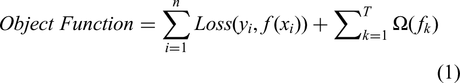
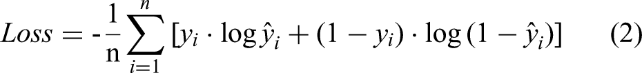
The traditional GBDT uses a depth-based splitting strategy (Level-wise) to split all leaves in the current layer simultaneously, resulting in lower computational efficiency and greater consumption of working memory. LightGBM adopts a leaf-wise splitting strategy, selecting the leaf with the greatest gain for splitting each time, maximising the depth of the tree and thus improving the model's accuracy and running speed, as shown in Figure 1. To further reduce the model's computational load and prevent overfitting, LightGBM also introduces the following improvements during the iterative solution process:

Histogram. The histogram algorithm is used to discretise continuous feature values. Based on the discretised features, a histogram is constructed to approximate the sample distribution. The split point with the largest gain is selected for splitting, which improves speed while mitigating overfitting.

Gradient-based One-Side Sampling (GOSS). The GOSS algorithm sorts the samples based on the absolute value of the gradient, retains high-gradient samples while sampling low-gradient samples, reducing redundant computations during model training and improving training speed.

Exclusive Feature Binding (EFB). By bundling features with certain correlations into exclusive feature groups, EFB can reduce the dimensionality and complexity of the model, lower the risk of overfitting and further enhance the model's generalisation ability.

Figure 1.

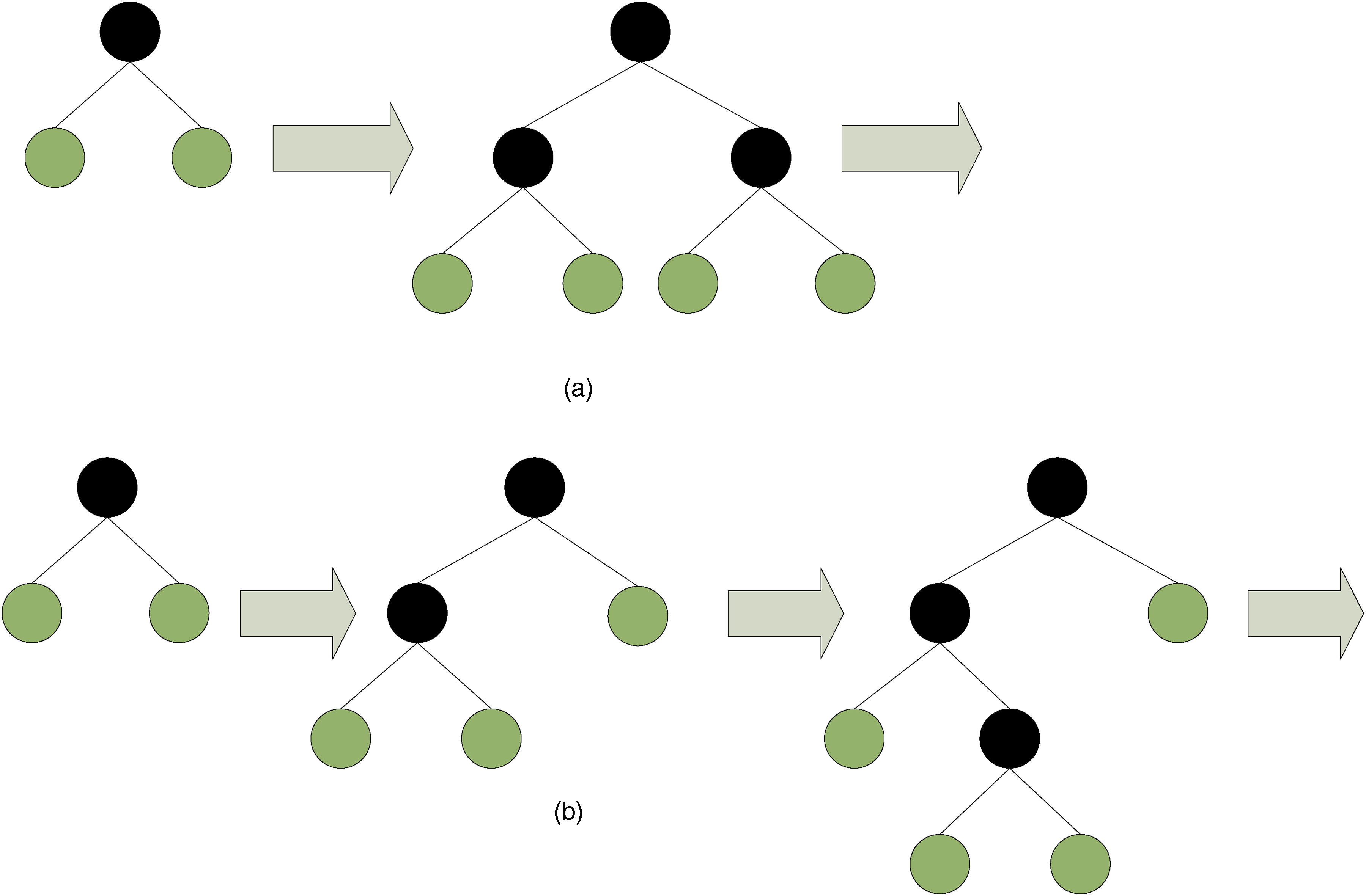
Decision tree split schematic: (a) level-wise split strategy; (b) leaf-wise split strategy.

Bayesian optimisation algorithm

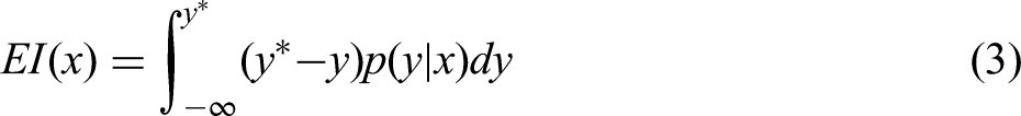
Bayesian optimisation algorithm^19–21 is a global optimisation algorithm based on probability distribution. Compared with traditional grid search or random search, Bayesian parameter optimisation can explore the parameter space more effectively and find a near-optimal parameter combination with relatively fewer attempts, thereby accelerating the training and tuning process of the model. Bayesian optimisation algorithm is mainly composed of two core parts: surrogate model and acquisition function. The surrogate model is generally divided into Gaussian process (GP) and tree-structured Parzen estimator (TPE); the acquisition function includes expected improvement (EI), probability of improvement (PI) and upper confidence bound (UCB). This paper uses the TPE algorithm provided by the Hyperopt library to estimate the relationship between parameter values and the objective function by establishing a tree-structured probability model. The probability model is dynamically adjusted and updated in each iteration, and the next more promising parameter value is selected for evaluation according to the objective function. The global optimal solution is found with as few iterations as possible, thereby reducing time and computational resources.

Expected improvement:

E I (x) = \int_{- \infty}^{y *} (y * - y) p (y | x) d y

(3)

Probability improvement:

P I (x) = \int_{- \infty}^{y *} p (y | x) d y

(4)

Confidence upper bound:

U C B (x) = μ (x) + κ σ (x)

(5)

where

y *

represents the current optimal target quantile threshold;

p (y | x)

represents the posterior probability of the current objective function;

μ (x)

represents the mean estimate of the objective function;

σ (x)

represents the variance estimate of the objective function;

κ

represents the hyperparameters that control exploration and search for equilibrium.

SHAP

Machine learning models have demonstrated impressive performance in various complex tasks, but their internal working mechanisms and decision-making processes are opaque. They typically operate as ‘black boxes.’ This ‘black box’ nature means that users cannot understand the internal decision-making process of machine learning models, the importance of feature parameters on decision outcomes, and the interactions between different feature parameters. This black box nature makes it difficult for people to understand how machine learning models make predictions or recommendations. In many fields where machine learning models are used, why such results are obtained is often as important as the results themselves.

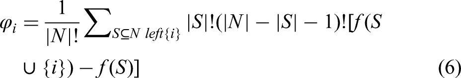
SHAP²² is an additive feature attribution model used to explain machine learning models. By calculating the SHAP values, the contribution of each feature to the model's prediction results is obtained, further quantifying the importance of each feature to the model. It is applicable to a variety of machine learning models.

Shapley values to each feature can be formulated as follows:

φ_{i} = \frac{1}{| N |!} \sum_{S \subseteq N l e f t {i}} | S |! (| N | - | S | - 1)! [f (S \cup {i}) - f (S)]

(6)

where N represents the set of features; S represents the feature subset after removing feature i;

f (S)

represents the model output of feature subset S;

f (S \cup {i}) - f (S)

represents the cumulative contribution value of feature i.

Model construction

Determination of the model input and output

The causes of the longitudinal crack are complex and mainly fall into two categories: the influence of molten steel composition and the impact of process factors. The influence of molten steel composition includes the content of carbon, phosphorus, sulphur, manganese, calcium, aluminum, micro-alloying elements and residual elements (arsenic, tin and copper) in the molten steel; the impact of process factors mainly includes the superheat degree of molten steel, casting speed, heat flow fluctuation of the mould, inlet temperature of cooling water of the mould, water flow rate of the mould, mould taper, fluctuation of mould level, electromagnetic brake of the mould, structure and insertion depth of the submerged nozzle, viscosity and alkalinity of the mould flux, thickness of the liquid slag layer, etc. In addition, operations such as protective casting, casting start, changing the tundish, changing the nozzle, changing the slag line also affect the occurrence of the longitudinal crack. This paper takes formation mechanism of the longitudinal crack on the slab surface and equipment-related factors^23,24 as the research background, combines the production process of a steel plant's continuous caster, analyses and mines historical production data, and selects 45 parameters such as the main element content in molten steel, casting speed, mould level, north taper and south taper, mould vibration frequency, negative slip time of mould vibration, mould thickness, inlet temperature of cooling water for the mould, etc. as model inputs, with the presence or absence of the longitudinal crack as model outputs.

Data preparation

Data collection and pre-processing

Using three months’ historical production data of the continuous caster in a steel plant as the original sample, all valid sample data of longitudinally cracked slabs and normal slabs were obtained by data cleaning, such as incomplete and abnormal slab sample data with variables exceeding the range were eliminated. The task of predicting longitudinal crack on the slab surface was transformed into a binary classification task in machine learning, with the relevant factors affecting the longitudinal crack as the model input and whether the slab has longitudinal crack as the model output. Here, considering that the incidence of longitudinal crack in actual production is very low, it is not graded according to its severity, and even if it is graded, its operation is relatively difficult. At present, it can only be divided into two categories according to whether longitudinal crack occur or not.

After data pre-processing, a total of 22,953 valid samples of normal slabs were labelled as class 0, and 35 valid samples of longitudinally cracked slabs were labelled as class 1, for a total of 22,988 samples. The distribution diagrams and descriptive statistics (maximum, minimum, mean, standard deviation, skewness and kurtosis) of each feature variable are shown in Figure 2. Among them, skewness is used to determine the symmetry of the data, and kurtosis is used to determine the steepness of the data distribution. When skewness is less than 0, the probability distribution is left-skewed, and when skewness is greater than 0, the probability distribution is right-skewed. When kurtosis is greater than 3, the peak is sharp, and when kurtosis is less than 3, the peak is flat. When skewness is 0 and kurtosis is 3, the feature completely follows a normal distribution.

Figure 2.

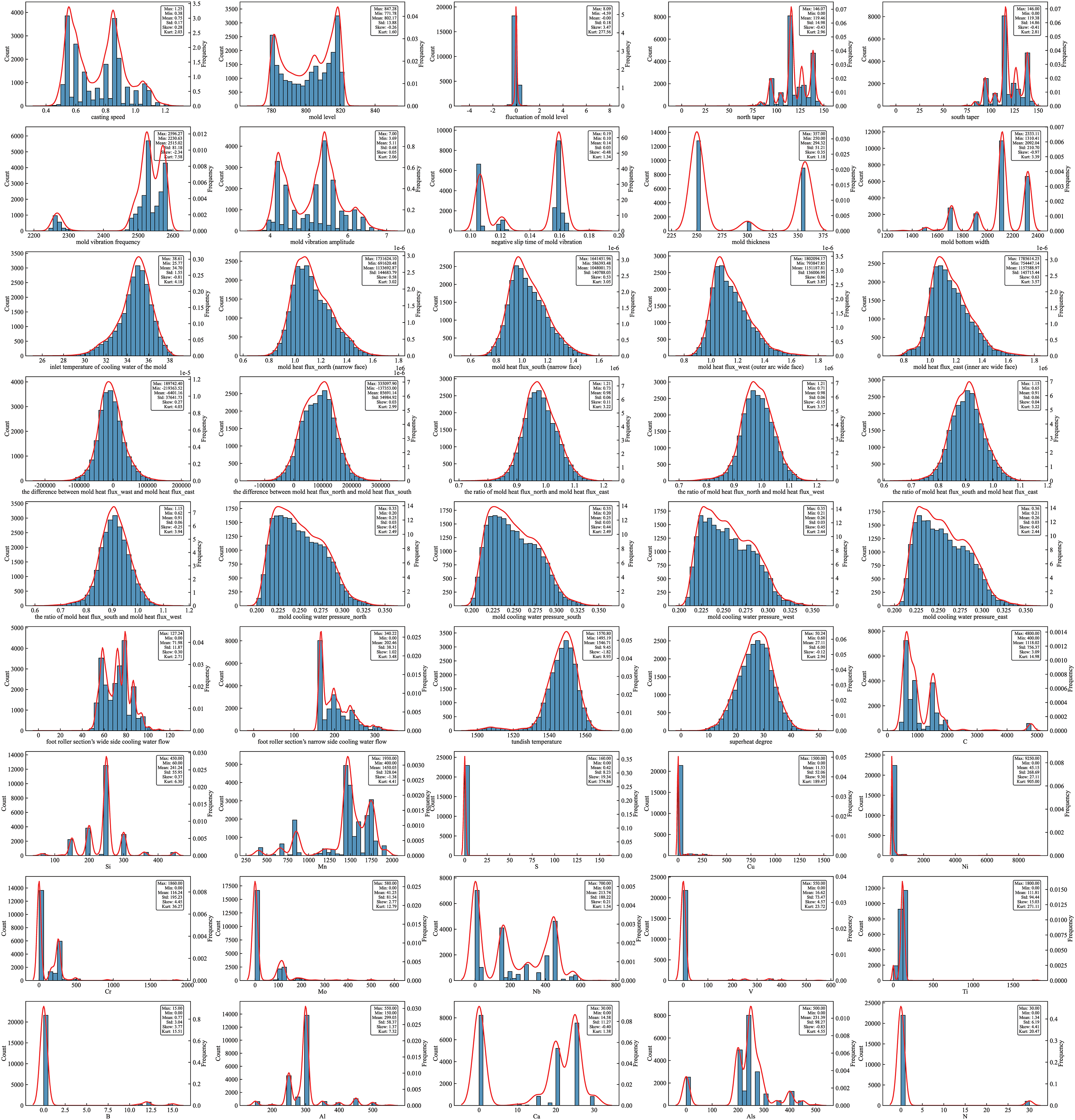
Histograms of the 45 variables in the final dataset.

As can be seen from Figure 2, some features exhibit multi-peak distribution, with multiple different values in the dataset. Some features exhibit long-tailed distribution, with most data concentrated in a smaller range and a small amount of data distributed in a larger range. In addition, only some of the remaining unimodal distribution features satisfy the normal distribution, with few features in the entire dataset that satisfy the normal distribution. Machine learning algorithms implicitly or explicitly assume that the data satisfies a normal distribution on a mathematical basis, enabling the algorithm to more accurately capture data features and thus improve model training and prediction performance. This paper uses a dataset where only a small number of features satisfy the normal distribution and the distribution of data categories is extremely imbalanced, which poses significant difficulties for subsequent modelling and prediction. At the same time, the distribution dimensions of each variable in the dataset vary greatly. If directly placed in the model for training, the excessive range difference will have a negative impact on the training and performance of the algorithm model to a certain extent.

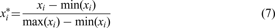
Normalise the data and convert the original data to the [−1, 1], by scaling the eigenvalues to fall within a relatively small range, improve the convergence speed of the optimisation algorithm, maintain the relative importance of different features, enhance the stability of the model and the ability to generalise, and further reduce the amount of model calculations to enhance the model accuracy, the formula is as follows:

x_{i} * = \frac{x_{i} - \min (x_{i})}{\max (x_{i}) - \min (x_{i})}

(7)

where

x_{i}

and

x_{i} *

represent data values before and after normalisation,

\max (x_{i})

and

\min (x_{i})

are the maximum and minimum values of the ith variable, respectively.

Imbalanced data processing

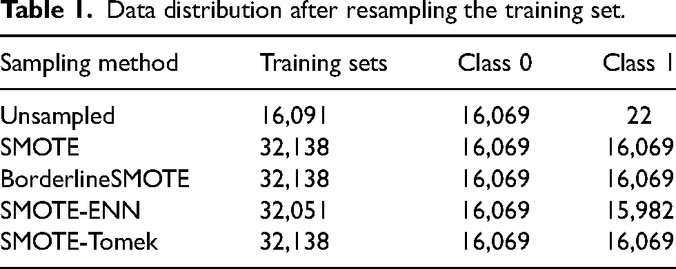
Due to the limited data of longitudinally cracked slabs in actual production and the existence of missed inspections and records, there is a serious imbalance in the effective sample data. There are a total of 22988 samples in this dataset, including 22953 effective samples of normal slabs and 35 effective samples of longitudinally cracked slabs. The ratio of effective samples of normal slabs to longitudinally cracked slabs is as high as 656:1, and the proportion of positive and negative samples is seriously imbalanced. The dataset is divided into a ratio of 7:3, with a total of 16,091 samples in the training set, including 16,069 normal slabs and 22 longitudinally cracked slabs; and a total of 6897 samples in the test set, including 6884 normal slabs and 13 longitudinally cracked slabs. The imbalance of data categories in the training set tends to interfere with the modelling process of the model, and resampling techniques are used to change the data distribution of the training set samples to achieve the purpose of balancing categories. This paper uses four sampling methods, namely SMOTE, BorderlineSMOTE, SMOTE-ENN and SMOTE-Tomek, to deal with imbalanced data, effectively eliminating the imbalance and achieving the balance of the categories. The data distribution after sampling in the training set is shown in Table 1.

Table 1.

Data distribution after resampling the training set.

Sampling method	Training sets	Class 0	Class 1
Unsampled	16,091	16,069	22
SMOTE	32,138	16,069	16,069
BorderlineSMOTE	32,138	16,069	16,069
SMOTE-ENN	32,051	16,069	15,982
SMOTE-Tomek	32,138	16,069	16,069

Modelling, training and optimisation

As shown in Figure. 3, the building process of longitudinal crack prediction model based on resampling and Bayesian optimised LightGBM consists of the following four main parts:

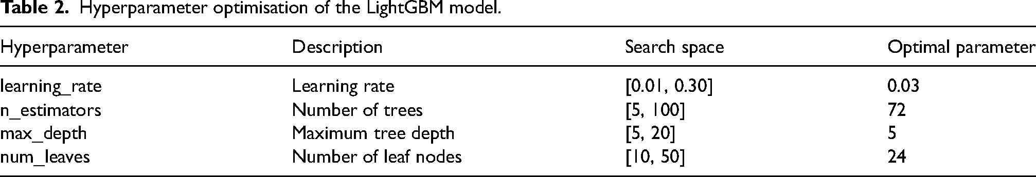
Data preparation and pre-processing. Collect and sort out massive continuous casting data on site. Then data pre-processing is carried out, including cleaning abnormal data, marking the binary classification labels, data normalisation processing, etc. And the preprocessed data is randomly divided into training set and test set.

Resampling. In order to alleviate the influence and interference of the unbalanced samples in the modelling process, two types of sampling methods, oversamping (SMOTE and BorderlineSMOTE) and mixed sampling (SMOTE-ENN and SMOTE-Tomek), are used to balance the training set and reduce the bias of the model to most categories.

Modelling and training of LightGBM. The training set after resampling is input into LightGBM for modelling and training. Based on CART regression tree, LightGBM model builds a new CART regression tree by iterating the residual of the previous tree. At the same time, the weight of leaf nodes is calculated, and the modified value of each tree is weighted to the current predicted value. Finally, the model outputs the weighted cumulative result of all CART regression trees.

Hyperparameter optimisation. The LightGBM model involves a lot of hyperparameters, and inappropriate hyperparameters will cause overfitting of the model. In this paper, Bayesian optimisation is used to optimise the hyperparameters of the model, the search range of hyperparameters is initialised, the optimal parameter combination is iteratively searched in the parameter space, and the average value of each group of hyperparameters is taken as the evaluation index by means of 5-fold cross-validation. The obtained optimal hyperparameters of the model are shown in Table 2.

Figure 3.

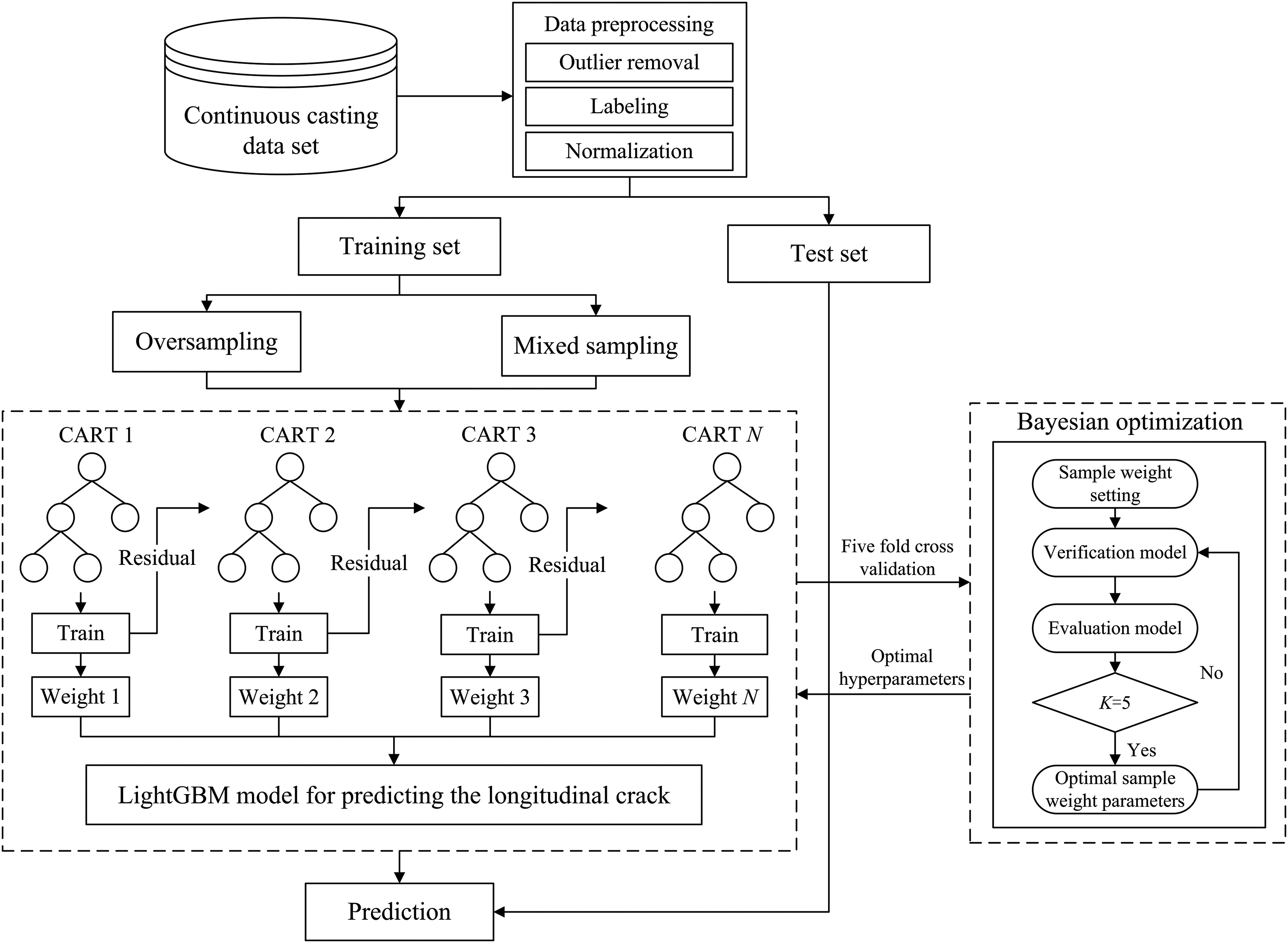
Flow of longitudinal crack prediction model based on resampling and Bayesian optimised LightGBM.

Table 2.

Hyperparameter optimisation of the LightGBM model.

Hyperparameter	Description	Search space	Optimal parameter
learning_rate	Learning rate	[0.01, 0.30]	0.03
n_estimators	Number of trees	[5, 100]	72
max_depth	Maximum tree depth	[5, 20]	5
num_leaves	Number of leaf nodes	[10, 50]	24

The prediction model of slab surface longitudinal cracks is established according to the optimal hyperparameters. The prediction experiment and comparison are carried out on the test set.

Model evaluation metrics

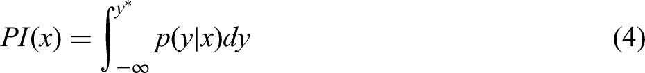
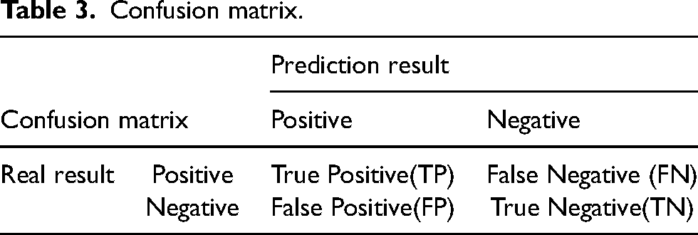
In this data set for this study, the imbalance ratio between the number of normal slab samples and the number of longitudinally cracked slab samples reached 656:1. For the binary classification problem of such unbalanced data, Accuracy alone cannot effectively and comprehensively measure the advantages and disadvantages of models. Therefore, Accuracy, Recall and False Alarm Rate (FAR) were introduced to comprehensively evaluate the prediction ability of the model, as shown in equations (8) to (11). The corresponding confusion matrix is shown in Table 3. Here, TP indicates that the reality is a positive example and the model classification result is also a positive example. FP indicates that the reality is a negative example and the model classification is a positive example. FN indicates that the reality is a positive example and the model classification is a negative example. TN indicates that the reality is a negative example and the model classification result is also a negative example. Recall_0 and Recall_1 are Recall of class 0 and class 1, respectively. The Recall actually reflects the prediction hit ratio. From equations (10) and (11), the sum of Accuracy and FAR is 1. For the prediction model of longitudinal crack, the two most concerned metrics are the prediction hit ratio of the longitudinal crack class (Recall_1) and FAR. The higher the Recall_1, the more longitudinal cracks can be detected. The higher the FAR, the higher the accuracy of the model's predictions for all classes.

Table 3.

Confusion matrix.

Confusion matrix		Prediction result
Confusion matrix		Positive	Negative
Real result	Positive	True Positive(TP)	False Negative (FN)
Real result	Negative	False Positive(FP)	True Negative(TN)

In addition, there is an evaluation metric of the model called AUC. AUC is the area under the receiver operating characteristics (ROC) curve, which quantifies a model's ability to distinguish between positive and negative samples. A higher AUC value indicates better classifier performance, whereas a value closer to 0.5 indicates poorer classifier performance. The ROC curve and AUC value are more focused on evaluating the overall performance of the model and are more suitable for assessing classifier capabilities in imbalanced datasets.

Recall_0 = \frac{T N}{T N + F P}

(8)

Recall_1 = \frac{T P}{T P + F N}

(9)

Accuracy = \frac{T P + T N}{T P + T N + F P + F N}

(10)

FAR = \frac{F P + F N}{T P + T N + F P + F N}

(11)

Simulation experiment

Experimental results and analysis

This paper uses four sampling methods, namely SMOTE, BorderlineSMOTE, SMOTE-ENN and SMOTE-Tomek, to process the original training set, and establishes slab surface longitudinal crack prediction models based on SVM, LR, RF, XGBoost and LightGBM, respectively, under the same experimental environment. The best combination of sampling method and prediction model is identified. The comparative experimental results are shown in Table 4. Here, the experimental environment used is the Windows 11 64-bit operating system, the CPU uses Inter(R) Core(TM) i7-12700H, the memory is 16G, and the graphics card is RTX-3060. The models are implemented using the Scikit-learn, LightGBM and Hyperopt libraries in Python, and the code compilation is done using Jupyter Notebook.

Table 4.

Comparison experiment results.

Model	Sampling method	Recall_0	Recall_1	Accuracy	FAR
SVM	Unsampled	100.00%	0.00%	99.81%	0.19%
	SMOTE	79.08%	84.62%	79.09%	20.91%
	BorderlineSMOTE	99.81%	23.08%	99.67%	0.33%
	SMOTE-ENN	92.02%	76.92%	92.00%	8.00%
	SMOTE-Tomek	91.98%	76.92%	91.95%	8.05%
LR	Unsampled	100.00%	0.00%	99.81%	0.19%
	SMOTE	90.67%	69.23%	90.63%	9.37%
	BorderlineSMOTE	97.82%	15.38%	97.67%	2.33%
	SMOTE-ENN	90.43%	76.92%	90.40%	9.60%
	SMOTE-Tomek	90.62%	76.92%	90.59%	9.41%
RF	Unsampled	100.00%	0.00%	99.81%	0.19%
	SMOTE	99.97%	15.38%	99.81%	0.19%
	BorderlineSMOTE	100.00%	0.00%	99.81%	0.19%
	SMOTE-ENN	99.90%	15.38%	99.74%	0.26%
	SMOTE-Tomek	99.93%	15.38%	99.77%	0.23%
XGBoost	Unsampled	100.00%	0.00%	99.81%	0.19%
	SMOTE	83.44%	69.23%	83.41%	16.59%
	BorderlineSMOTE	99.96%	0.00%	99.77%	0.23%
	SMOTE-ENN	99.87%	15.38%	99.71%	0.29%
	SMOTE-Tomek	99.83%	15.38%	99.67%	0.33%
LightGBM	Unsampled	99.97%	0.00%	99.78%	0.22%
	SMOTE	90.57%	84.62%	90.56%	9.44%
	BorderlineSMOTE	99.97%	0.00%	99.78%	0.22%
	SMOTE-ENN	99.80%	23.08%	99.65%	0.35%
	SMOTE-Tomek	98.85%	38.46%	98.74%	1.26%

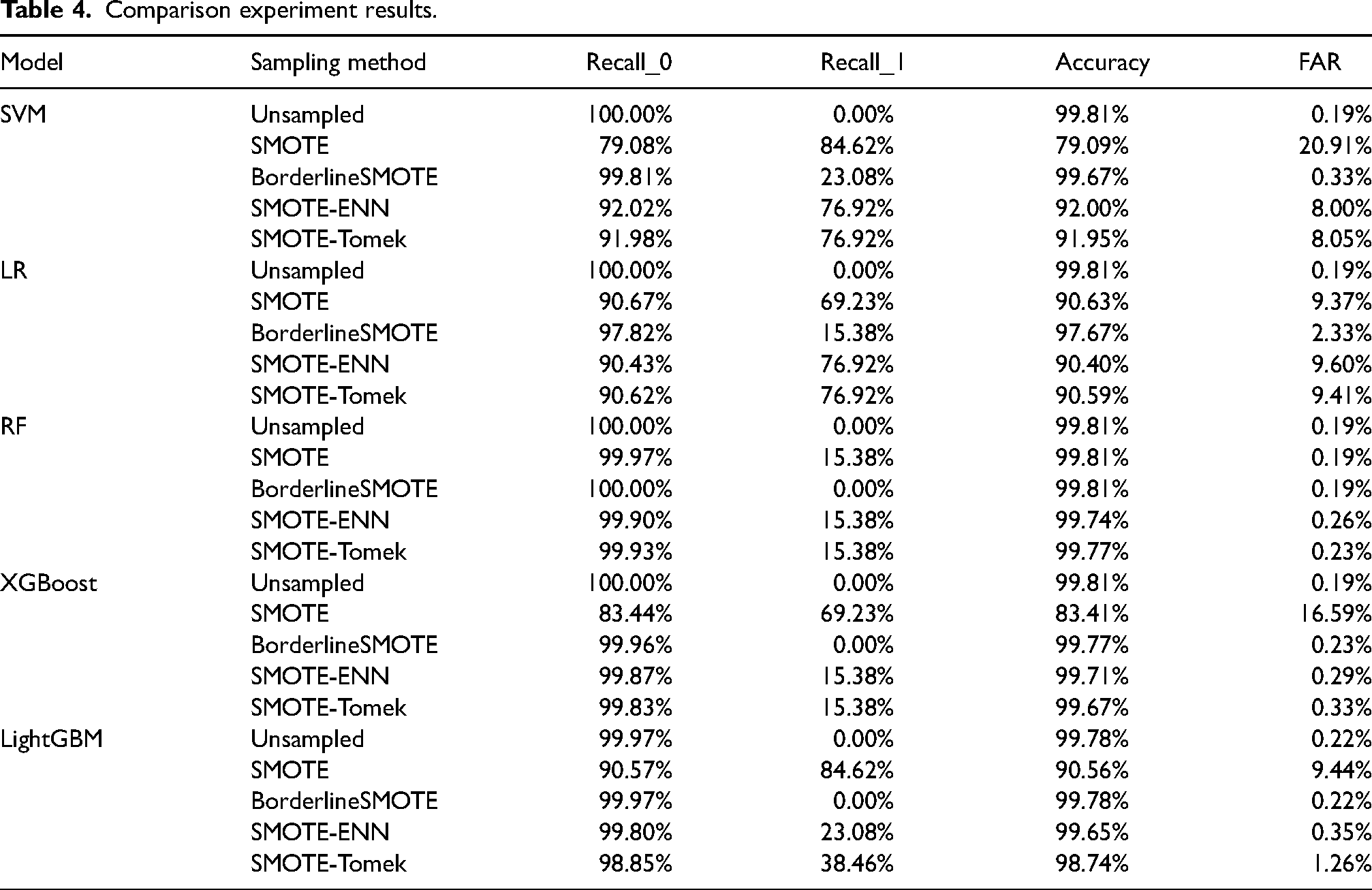
As shown in Table 4, the SVM, LR, RF, XGBoost and LightGBM models achieved an impressive Accuracy of 99.81% on the original dataset, yet their Recall_1 values were all 0, indicating an inability to accurately predict longitudinally cracked slabs. The models’ predictive capabilities for longitudinally cracked slabs significantly improved after employing resampling techniques. Among them, the LightGBM_SMOTE model demonstrated the best predictive performance post-resampling, followed by the SVM_SMOTE and LR_ SMOTE-ENN models. Their evaluation metrics are depicted in Figure 4. Both the SVM_SMOTE and LightGBM_SMOTE models achieved a prediction accuracy of 84.61% for defective slabs, while the LR_SMOTE-ENN model's prediction accuracy was 76.92%. Notably, the SVM_SMOTE model had a slightly lower prediction accuracy of 79.08% for normal slabs.

Figure 4.

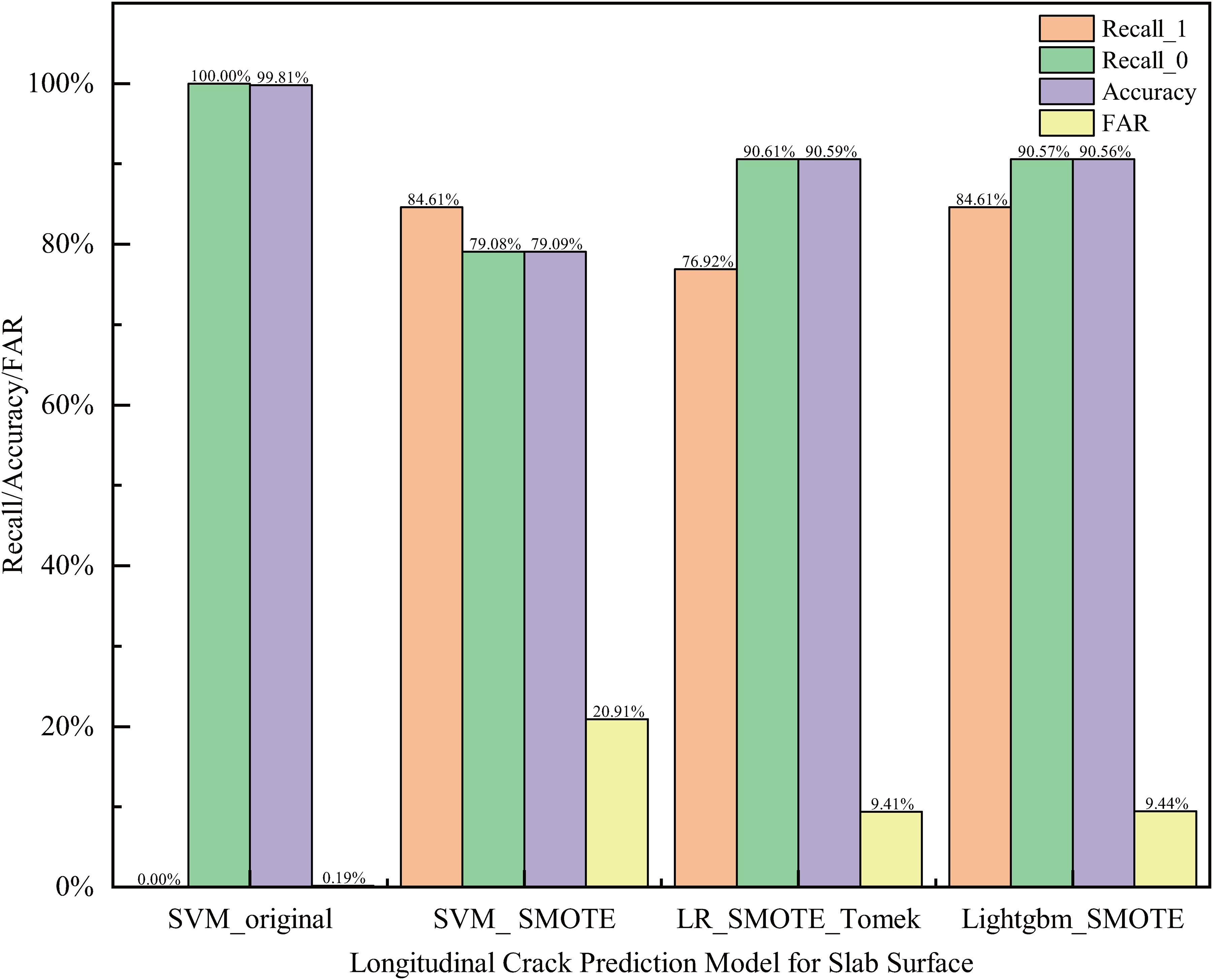
Evaluation of longitudinal crack prediction models.

The ROC curve is illustrated in Figure 5. From Figure 5, the AUC value for the SVM_SMOTE model was relatively low at 0.88, whereas the AUC value for the LR_SMOTE-ENN model was 0.90, indicating a slight improvement of 0.02 compared to the SVM_SMOTE model, suggesting that both the SVM_SMOTE and LR_SMOTE-ENN models have similar predictive capabilities. Among them, the LightGBM_SMOTE model had the highest AUC value at 0.93, capturing more complex data patterns and relationships compared to the SVM_SMOTE and LR_SMOTE-ENN models.

Figure 5.

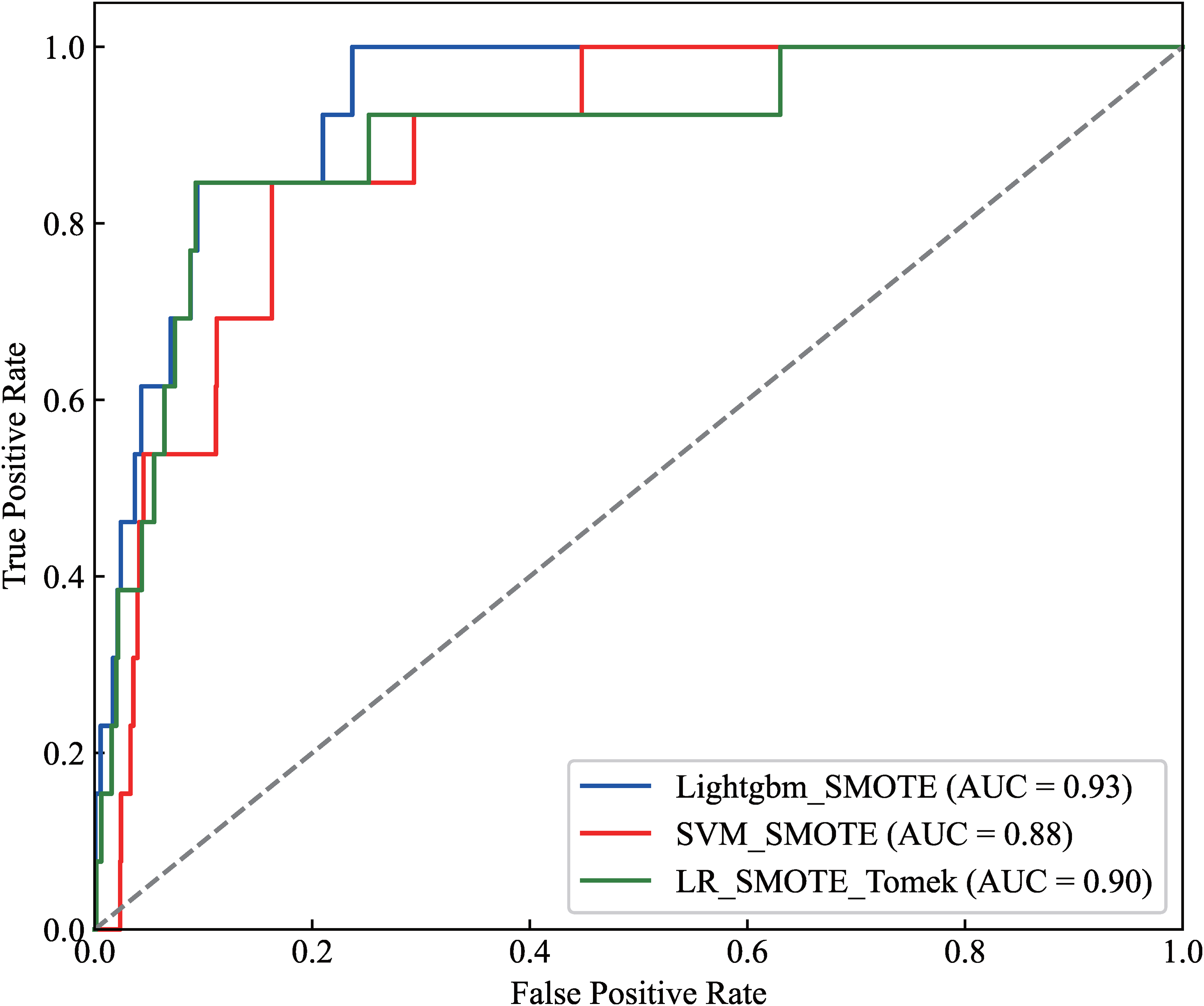
ROC curve of longitudinal crack prediction model on slab surface.

Comparing the training time and prediction time of the above-mentioned superior models, it was found that the SVM_SMOTE model took the longest training time of 23.25 s and a prediction time of 8.88 s. The LR_SMOTE_Tomek model had a training time of 0.16 s and a prediction time of 0.01 s, which was a significant improvement compared to the SVM_SMOTE model. The Lightgbm_SMOTE model adopted histogram, one-sided gradient sampling and mutually exclusive feature binding strategies, which enabled it to quickly process massive data, with faster training speed and lower memory consumption. Its training time was about 0.15 s and prediction time is less than 0.01 s. The time consumed in each stage for the Lightgbm_SMOTE model is significantly shorter than other models. As can be seen from the above analysis, the Lightgbm_SMOTE shows obvious advantages in the prediction of the longitudinal crack on the slab surface.

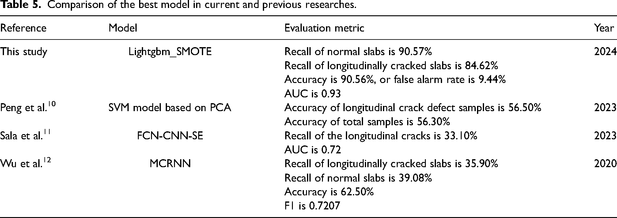
Furthermore, as for the slab surface longitudinal crack prediction models driven by data of the main influencing factors, the prediction performances of the previous researches and the best model in this study are compared, as shown in Table 5. From Table 5, the LightGBM_SMOTE model outperforms other models in prediction accuracy. Compared with other models, the Recall, Accuracy and AUC of the LightGBM_SMOTE model have been greatly improved. The improvement of the new model proposed by this study is mainly due to the full consideration of the extreme imbalance in longitudinal crack samples, and the combination optimisation of multiple resampling methods and classification algorithms. Therefore, it can capture more complex data patterns and relationships, effectively improving the prediction accuracy of longitudinally cracked slabs while maintaining the accuracy of normal slabs.

Table 5.

Comparison of the best model in current and previous researches.

Reference	Model	Evaluation metric	Year
This study	Lightgbm_SMOTE	Recall of normal slabs is 90.57%	2024
		Recall of longitudinally cracked slabs is 84.62%
		Accuracy is 90.56%, or false alarm rate is 9.44%
		AUC is 0.93
Peng et al.¹⁰	SVM model based on PCA	Accuracy of longitudinal crack defect samples is 56.50%	2023
Peng et al.¹⁰	SVM model based on PCA	Accuracy of total samples is 56.30%	2023
Sala et al.¹¹	FCN-CNN-SE	Recall of the longitudinal cracks is 33.10%	2023
Sala et al.¹¹	FCN-CNN-SE	AUC is 0.72	2023
Wu et al.¹²	MCRNN	Recall of longitudinally cracked slabs is 35.90%	2020
		Recall of normal slabs is 39.08%
		Accuracy is 62.50%
		F1 is 0.7207

Model interpretation and analysis based on SHAP values

An interpretative analysis was conducted on the LightGBM_SMOTE model based on SHAP, and the summary plot of feature importance is shown in Figure 6. The positions of sample points on the y-axis and x-axis correspond to feature values and SHAP values, respectively. The color of the points ranges from blue to red, indicating that feature values range from low to high. Positive and negative SHAP values indicate the positive and negative correlations between feature variables and output results. A positive correlation, where the SHAP value is positive, promotes the occurrence of the longitudinal crack, while a negative correlation, where the SHAP value is negative, inhibits the occurrence of the longitudinal crack. The figure shows that the inlet temperature of cooling water for the mould, the foot roller section's narrow side cooling water flow, the mould heat flux_south (narrow face), the C element content, the mould heat flux_north (narrow face), the fluctuation of mould level, the foot roller section's wide side cooling water flow and the ratio of mould heat flux_south and mould heat flux_west are the main influencing factors affecting the longitudinal crack. The quantitative analysis of the above important influencing factors and longitudinal crack defects is shown in Figure 7.

Figure 6.

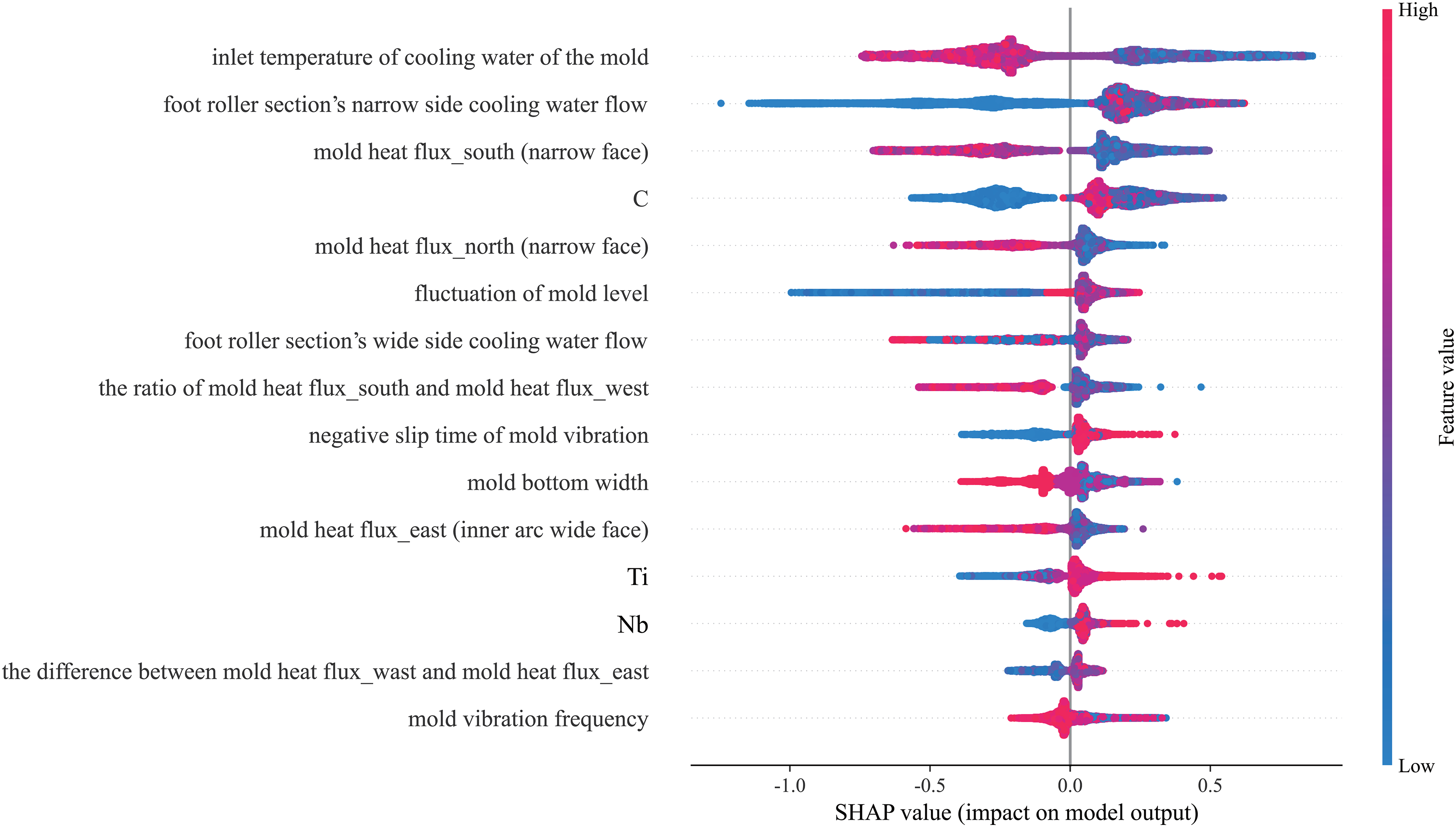
Summary chart of the importance of SHAP features.

Figure 7.

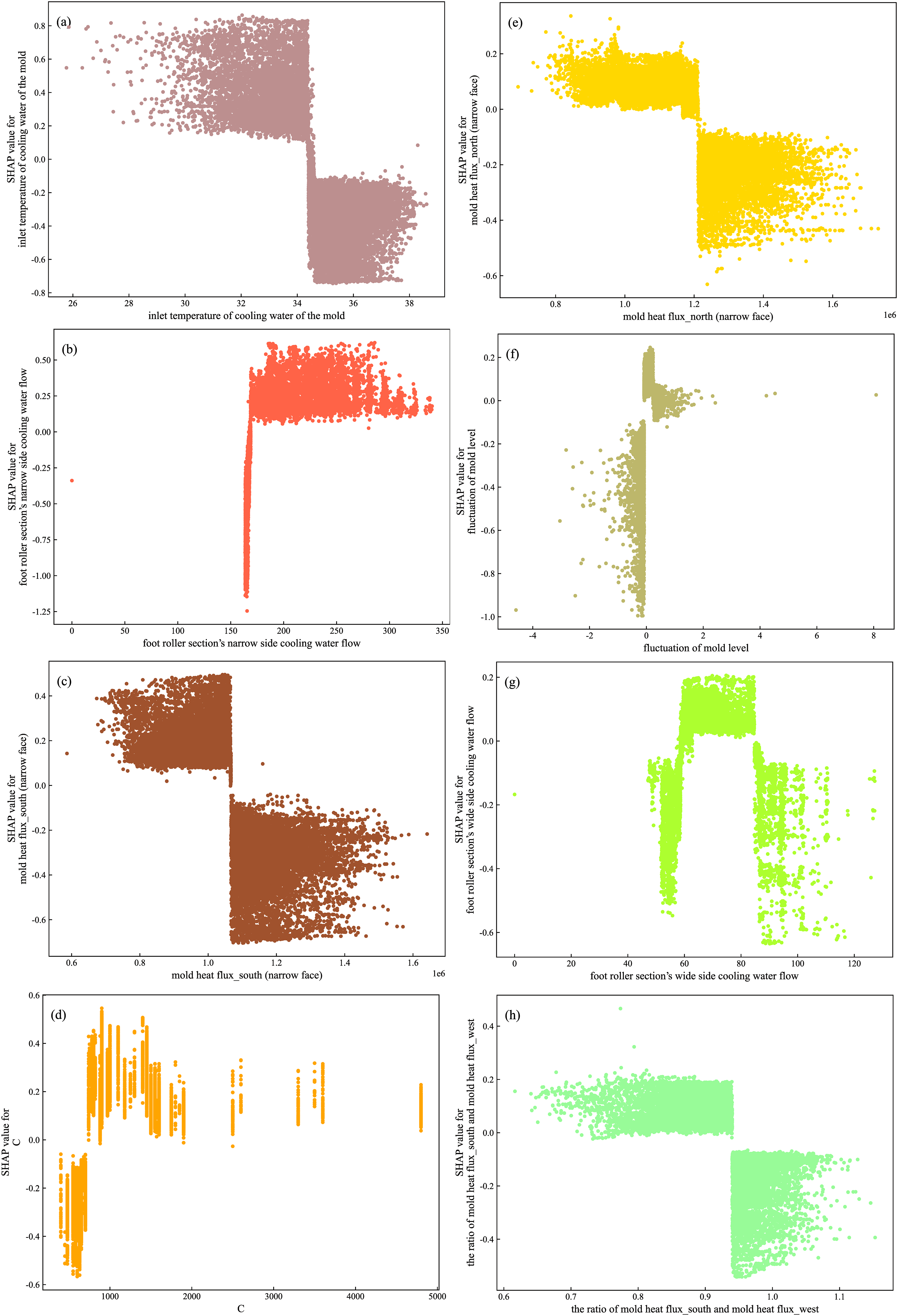
Dependency diagram of important characteristics and target characteristics.

Surface defects in slabs originate from the initial solidification stage of the molten steel, influenced by heat transfer between the molten steel and the cooling copper mould, initial solidification of the molten steel, and the physicochemical properties of the selected mould flux. In particular, the heat transfer uniformity during the initial solidification process of the molten steel and the uniform growth of the shell have a significant impact. Changes in the composition of the molten steel affect its heat transfer efficiency or solidification efficiency, as well as its high-temperature phase transformation process. Continuous casting parameters are also an important factor affecting uniform heat transfer in the mould.^23–27 The molten steel contains various elements such as C, P, S and Mn, among which the C content has a significant impact on the sensitivity of surface cracks of the slab. When the C content is between 0.09% and 0.17%, the peritectic reaction L + δ → γ during the solidification process of the molten steel is intense, leading to a significant change in the linear contraction of the solidified shell. When the linear contraction reaches a certain level, the air gap between the continuous casting slab shell and the mould becomes larger, leading to the occurrence of depressions. At the same time, the heat flow decreases, the primary shell becomes thinner, and under the action of thermal stress and other stresses, the crack will form at the bottom of the depression. The incidence of the longitudinal crack with a C content between 0.11% and 0.14% is the highest. This paper uses a dataset in which peritectic steel accounts for the majority, with a C (>0.09%) and a positive SHAP value, promoting the occurrence of the longitudinal crack. The longitudinal crack is formed in the mould and are closely related to the cooling intensity of the mould. The cooling intensity can be divided into the influence of the mould heat flux, the ratio of mould heat flux and the temperature at the mould inlet. Uneven heat flux in the meniscus region of the mould can lead to uneven growth thickness of the shell, causing uneven transverse temperature gradients and generating transverse tensile stresses, which in turn lead to longitudinal cracks. Proper control of the mould heat flux, ratio of the mould heat flux and the inlet temperature of cooling water of the mould in the continuous casting process helps to suppress the formation of the longitudinal crack. As shown in Figure 7, the larger the mould heat flux_south (narrow face) (>1.05 × 10⁶), the larger the mould heat flux_north (narrow face) (>1.2 × 10⁶), the larger the ratio of mould heat flux_south and mould heat flux_west (>0.95), and the larger the inlet temperature of cooling water of the mould (>34.50), the smaller the SHAP value, which will inhibit the occurrence of the longitudinal crack.

In addition, the fluctuation of mould level and the secondary cooling water flow rate are also the main factors affecting the occurrence of the longitudinal crack. The longitudinal crack occurs in the meniscus area in the mould. Due to the support of the mould, the cracks will not expand. However, after the solidified shell leaves the mould, the excessive cooling of the foot roller and the zero section will increase the occurrence rate of the longitudinal crack. The adjustment of the cooling water volume in the secondary cooling zone should ensure that there is no leakage of steel from the mould, and should not be too strong to cause the growth of the crack. As shown in Figure 7, the larger the foot roller section's narrow side cooling water flow (>160), the positive SHAP value will promote the occurrence of the longitudinal crack; the larger the foot roller section’s wide side cooling water flow (>90) or the smaller the foot roller section’s wide side cooling water flow (<62), the negative SHAP value will inhibit the occurrence of the longitudinal crack. The large the fluctuation of mould level will destroy the stability of the liquid slag layer, affect the melting and lubrication of the mould flux, lead to uneven heat transfer in the mould, and increase the probability of the longitudinal crack. When the fluctuation of mould level is larger (>0.10), the positive SHAP value will promote the occurrence of the longitudinal crack.

Conclusions

Aiming at the unbalance problem of data set for longitudinal crack prediction, a method based on resampling and Bayesian optimisation of LightGBM was proposed in this paper. First, four sampling methods (such as SMOTE, BorderlineSMOTE, SMOTE ENN and SMOTE Tomek) were used to construct a class-balanced training set. Then, five classification algorithms (such as SVM, LR, RF, XGBoost and LightGBM) were combined to establish the prediction model of the longitudinal crack, and the optimal algorithm combination was selected. On this basis, SHAP is used for explanatory analysis of the model, to grasp the influence of each input feature on the model prediction results, so as to improve the transparency and reliability of the model. The main conclusions were as follows:

Compared with the original data set, SMOTE, BorderlineSMOTE, SMOTE-ENN and SMOTE-Tomk have improved the classification performance of five classification algorithms on the unbalanced data set to varying degrees. Furthermore, the data set processed by SMOTE sampling method has the best effect for subsequent classification, which can improve the prediction accuracy of longitudinally cracked slabs effectively.

By comparing the model combinations of various sampling methods and classification algorithms, it is found that LightGBM_SMOTE model is significantly better than other models on the test set, and its prediction accuracy for normal slabs and longitudinally cracked slabs are 84.62% and 90.57%, respectively, and the AUC is 0.93. At the same time, the training time and prediction time of LightGBM_SMOTE model are 0.146 s and 0.006 s respectively, which indicates that the memory consumption is smaller and computational efficiency is higher. Taking many aspects into consideration, LightGBM_SMOTE shows obvious advantages in the prediction of the longitudinal crack.

The SHAP method is used to interpret the output of the model, and the influence factors of the longitudinal crack which are inputted into the model, were ranked in importance. The results show that the inlet temperature of the cooling water of the mould (>34.5), mould heat flux_south (narrow face) (>1.05 × 10⁶), mould heat flux_north (narrow face) (>1.2 × 10⁶) and the ratio of mould heat flux_south and mould heat flux_west (>0.95) were conducive to the suppression of the longitudinal crack. The results of C content (>0.09%), fluctuation of mould level (>0.1), the foot roller section's narrow side cooling water flow (>160) and foot roller section's wide side cooling water flow in the range of 62‒90 will promote the generation of the longitudinal crack, which are consistent with the theoretical and empirical knowledge, and improves the explanatory ability of the model prediction.

This paper proposes a method for predicting the longitudinal crack under the condition of unbalanced data. It uses the SMOTE sampling algorithm to alleviate the problem of sample imbalance, and then combines the LightGBM classification algorithm to establish the prediction model for the longitudinal crack. Compared with the traditional prediction method that did not consider the problem of longitudinal crack sample imbalance, the method improves the prediction accuracy of longitudinally cracked slabs while maintaining the accuracy of normal slabs. This study focuses on dealing with data imbalance problems and improving the performance of prediction model, but it is still insufficient in the generalisation of sampling algorithms and in-depth mining of feature engineering. The next step of research can focus on multi-source data fusion and dynamic feature construction. model, optimise feature engineering and sampling strategies, and carry out online testing and application verification in industrial sites.

Footnotes

Acknowledgements

The authors are grateful to the financial support for the Anhui Provincial Education Department Natural Science Research Project (Grant No. 2022AH050293) and the National Natural Science Foundation of China (Grant No. 52204330).

Author contributions

Fei He contributed to paper idea, project administration, supervision and writing–review and editing. Xinyao Wang contributed to investigation, validation and writing–original draft preparation. Yan Yu contributed to methodology, resources and supervision. Xufeng Liu contributed to formal analysis and methodology. JunQiang Cong contributed to investigation. Quanjun Wu contributed to assistance in the experiment. Yingjie Song contributed to assistance in the experiment. All the authors contributed to the final manuscript.

Declaration of conflicting interests

The authors declared no potential conflicts of interest with respect to the research, authorship and/or publication of this article.

Funding

The authors disclosed receipt of the following financial support for the research, authorship and/or publication of this article: This work was supported by the Anhui Provincial Education Department Natural Science Research Project (2022AH050293), National Natural Science Foundation of China (52204330).

ORCID iD

Fei He

References

Zhou

Luo

. Some considerations for digitization development of high-efficiency continuous casting. Metall Ind Autom 2023; 47: 68–85.

Jin

. Predictions of steel price indices through machine learning for the regional northeast Chinese market. Neural Comput Appl 2024; 36: 20863–20882.

Zhang

. Price forecasts of ten steel products using Gaussian process regressions. Eng Appl of Artif Intell 2023; 126: 106870.

Poltarak

Ferro

Cicutti

. Estimation of internal cracking risk in the continuous casting of round bars. Steel Res Int 2017; 88: 1600223.

Wang

Liu

, et al. Prediction of longitudinal cracks based on a full-scale finite-element model coupled inverse algorithm for a continuously cast slab. Steel Res Int 2017; 88: 1700013.

Wang

Cai

, et al. Calculation of continuous casting billet solidification based on element-free Galerkin method. Chin J Eng 2020; 42: 186–193.

Liu

Wang

Sun

, et al. Research on a new detection method of slab surface crack in mould during continuous casting. Metall Res Technol 2018; 115: 1–6.

Duan

Wei

, et al. Longitudinal crack detection approach based on principal component analysis and support vector machine for slab continuous casting. Steel Res Int 2021; 92: 2100168.

Zhang

Duan

Wang

, et al. Longitudinal crack predition method of continuous cast slab based on random forest and clustering. Continuous Casting 2022; 6: 21–28.

10.

Peng

Hou

, et al. Correlation between longitudinal crack occurrence and mold heat transfer in continuous casting based on process data mining. J Iron Steel Res Int 2024; 31: 1139–1152.

11.

Sala

Van Yperen-De Deyne

Mannens

, et al. Hybrid-input FCN-CNN-SE for industrial applications: classification of longitudinal cracks during continuous casting. Metals 2023; 13: 1699.

12.

Jin

, et al. Multiscale convolutional and recurrent neural network for quality prediction of continuous casting slabs. Processes 2020; 9: 33.

13.

Gong

Kim

. RHSBoost: improving classification performance in imbalance data. Comput Stat Data Anal 2017; 111: 1–13.

14.

Devi

Biswas

Purkayastha

. Redundancy-driven modified Tomek-link based undersampling: a solution to class imbalance. Pattern Recog Lett 2017; 93: 3–12.

15.

Shen

Nie

, et al. A hybrid sampling algorithm combining M-SMOTE and ENN based on random forest for medical imbalanced data. J of Biomed Inf 2020; 107: 103465.

16.

Chawla

Bowyer

Hall

, et al. SMOTE: synthetic minority over-sampling technique. J Artif Intell Res 2002; 16: 321–357.

17.

Al Majzoub

Elgedawy

Akaydın

, et al. HCAB-SMOTE: a hybrid clustered affinitive borderline SMOTE approach for imbalanced data binary classification. Arabian J Sci Eng 2020; 45: 3205–3222.

18.

Zeng

Yang

Zhang

, et al. A LightGBM-based EEG analysis method for driver mental states classification. Comput Intell Neurosci 2019; 2019: 1–11.

19.

Wang

Zhang

, et al. Prediction of final cooling temperature for hot rolled plate based on Bayesian optimized LightGBM. Metall Ind Autom 2024; 48: 54–64.

20.

Sultana

Hossain

SMZ

Abusaad

, et al. Prediction of biodiesel production from microalgal oil using Bayesian optimization algorithm-based machine learning approaches. Fuel 2022; 309: 122184.

21.

Deng

Zhu

, et al. Forecasting carbon price trends based on an interpretable light gradient boosting machine and Bayesian optimization. Expert Syst Appl 2024; 242: 122502.

22.

Scott

Su-In

. A unified approach to interpreting model predictions. Adv Neural Inf Process Syst 2017; 30: 4765–4774.

23.

Zhang

Chen

Zhang

, et al. Dynamic spray cooling control model based on the tracking of velocity and superheat for the continuous casting steel. J of Mater Process Technol 2016; 229: 651–658.

24.

Wang

Zhu

Zhou

. Initial solidification and its related heat transfer phenomena in the continuous casting mold. Steel Res Int 2017; 88: 1600488.

25.

Liu

Cheng

. Study of crack sensitivity of peritectic steels. Coatings 2021; 12: 15.

26.

Wang

Gao

, et al. Thin slab casting and direct rolling technology: current status and prospects. Chin J of Eng 2022; 44: 534–545.

27.

Wang

Zeng

, et al. Research status of the formation and control of surface longitudinal cracks during continuous casting. Continuous Casting 2024; 43: 1–7.