Research on key indicators prediction of steel process adapting to operating condition deviation

Abstract

This study developed an indicator prediction model for steel processes adapting to dynamic operating condition deviations. By combining just-in-time learning, ensemble learning techniques, and target similarity extraction, the model improves prediction accuracy and robustness. Validated on industrial rolling and sintering data, the model achieves up to 18% improvement over traditional models. Utilizing multi-dimensional parameters, the 6% error margin hit rates for yield and tensile strength reached 86% and 99% in rolling data, while the Al₂O₃ hit rate reached 96% in sintering. Notably, for boundary samples (top/bottom 25% quantiles), the model achieved a 56% relative improvement in hit rate. Furthermore, the model significantly enhances prediction robustness under dynamic operating deviations, reducing the accuracy fluctuation across time segments from 12% to 5%.

Keywords

Steel,operating condition deviation indicator prediction ensemble just-in-time learning boundary samples target

Introduction

The stage or end-point target variables involved in each process of steel production are called the key indicators of steel process, such as steel rolling quality,¹ sintering quality,² molten steel temperature,³ and so on. The real-time information of key indicators has a significant impact on improving product quality, reducing energy consumption, and improving production efficiency. However, the traditional detection and measurement methods often have the problems of time lag and high cost. Therefore, the prediction technology of key indicators of a steel process flow based on production process data came into being.^4,5 It can predict key indicators in advance, provide support for production decisions, and reduce maintenance and use costs.

The core challenges of the prediction technology for key indicators of an iron and steel process are focused on two aspects: data and models. One is to comprehensively and accurately collect the relevant influencing factors of indicators, and the other is to establish the model relationship between relevant factors and key indicators. At present, most researchers study and improve the model on the basis of high-quality data, and realise the accurate prediction of key indicators with the help of machine learning technology.⁶ Furthermore, an increasing number of studies have extensively explored the complex physical properties, micro-structural evolution, physical metallurgy, and accurate classification of various steel products using advanced analytical and machine learning technologies.^7–14 Li et al.¹⁵ propose a novel dynamic time feature expanding and extracting framework integrated with recurrent neural network regression to predict sinter quality in industrial processes. Shi et al.⁴ propose a data-driven furnace heat prediction and feedback model integrating genetic algorithm-enhanced machine learning with blast furnace metallurgical processes, achieving great accuracy for hot metal temperature and chemical heat prediction, while improving furnace temperature stability through industrial implementation.

In a broader context, advanced data-driven predictive frameworks have achieved widespread success in related metal processing and manufacturing fields, such as tube bending prediction and thermal error compensation.^16,17 Furthermore, foundational research continues to deeply explore complex physical metallurgical phenomena, such as the thermal stability of metastable austenite in steels.¹⁸ A large number of previous studies have directly established global indicators prediction models for historical datasets, and achieved good results in the experimental state. However, if it is applied to the practice of steel production, the model effect is likely to decline or drop sharply. The reason is that most of the production process parameters change with time in the industrial scenario, that is, the operating condition deviation.¹⁹ Operating condition deviation will lead to unpredictable changes in the data distribution after the training model. The production process parameter data presented when the model is applied to production does not correspond to the data distribution provided during the training. At the same time, the mapping relationship between the production process parameters and the target indicators will also change, resulting in a decline in the prediction ability of the model.²⁰

To address the unpredictability of data distribution shifts, the concept of just-in-time learning (JITL) is widely employed. Originally established in the late 1990s as a powerful ‘model-on-demand’ framework for anticipating time-series behaviour and facilitating process control,^21,22 JITL effectively mitigates the continuous drift of operating conditions by dynamically extracting a sample set similar to the current state from historical data for local modelling.²³ Furthermore, ensemble learning (EL)²⁴ has been introduced into these industrial scenarios to further enhance prediction accuracy by aggregating multiple models.

Recent advancements have further expanded JITL’s capabilities in industrial soft sensing by integrating it with robust representation learning and advanced autoencoders to handle complex, non-stationary data distributions.^25,26 Building on these modern frameworks, Shao et al.²⁷ introduced JITL into industrial soft sensing and optimised its performance by addressing sample selection bias and non-Gaussian distribution modelling challenges, achieving improved prediction accuracy. Dong et al.²⁸ combined JITL and EL technology, proposed a soft sensing method based on integrated local modelling to realise the just-in-time prediction of mechanical properties of hot rolled strips, and verified the effect of the model in the experiment. To effectively track shifting trends in both stable and transitional conditions, Song et al.²⁹ introduce JITL technology and propose a data-driven progressive search and parallel model framework, which rapidly predicts temperature during transition states in continuous annealing processes. By leveraging an ensemble framework, de Matos et al.³ achieved higher prediction accuracy for molten steel temperature than individual models, effectively modelling both linear and non-linear thermal loss patterns caused by dynamic variables. We designate this method as HLRFR and employ it in subsequent comparative experiments.

On the basis of existing research, this study combines EL with JITL to propose an ensemble learning-based just-in-time learning (EL-JITL) method. To improve it, inspired by recent optimisations of JITL similarity criteria in sintering processes,³⁰ we introduce the concept of target similarity. It predicts the target through the pseudo-label prediction model, limits the similar sample set of EL-JITL, and improves the prediction ability of the model for boundary samples. The main novelty and rationale of this work lie in overcoming the ‘feature–target decoupling’ phenomenon that inherently plagues standard global models and traditional distance-based JITL under dynamic operating condition deviations. Unlike existing models that rely solely on historical feature–space proximity, which can be highly misleading under industrial noise, our proposed framework introduces a pseudo-label-driven target similarity mechanism. By explicitly coupling this constraint with a multi-dimensional ensemble stacking strategy, the TS-EL-JITL method fundamentally reduces epistemic uncertainty and avoids over-smoothing. Ultimately, we propose the TS-EL-JITL method to further improve the robustness and accuracy of key indicator predictions in the steel process.

For clarity and ease of reference, all principal mathematical symbols and acronyms used throughout this paper are summarised in the Notation in the Appendix.

Methodology

The dynamic change and offset of production conditions cause the data distribution to change rapidly, which greatly restricts the effect of the traditional prediction model. The introduction of JITL for dynamic local modelling and prediction of current samples to be tested in the production process can alleviate the above problems to a certain extent. However, JITL uses a single similarity strategy to select the set of modelling samples from historical data, which has limitations for reflecting the characteristics of the current sample to be tested, and further limits the effect of the local prediction model.

In order to deal with the above technical difficulties, this study proposes an EL-JITL prediction method that integrates target similarity, named TS-EL-JITL. The method is divided into three stages: JITL, integrating target similarity and EL. Regarding the nomenclature, TS-EL-JITL is named following a descriptive modifier convention rather than strict chronological execution: JITL serves as the core foundational framework, while TS and EL are descriptive prefixes representing the two novel enhancement mechanisms applied to it. Firstly, a variety of similarity strategies are integrated to make up for the limitations of a single similarity strategy in capturing similarity and enhance the generalisation ability of the model. Secondly, the target similarity calculation module is introduced to evaluate the similarity between the target indicator and the historical data of the sample to be tested, and further optimise the set of similar samples, which plays a great role in improving the prediction effect of boundary samples. Finally, the EL idea is used to improve the overall accuracy and robustness of the model. This method not only improves the accuracy of prediction, but also enhances the adaptability of the model to the rapid change of production conditions. The overall model framework is shown in Figure 1.

Figure 1.

Framework of TS-EL-JITL. TS-EL-JITL: target-similarity ensemble just-in-time learning.

Next, the three stages will be described in detail. The historical data samples are represented by $(X, Y) = ((X_{1}, X_{2} \dots X_{n}), (Y_{1}, Y_{2} \dots Y_{n}))$ . $X$ denotes the feature set of historical data samples, while $Y$ represents their corresponding indicator labels, and $n$ is the number of historical data samples. The sample to be tested is represented by $X_{test}$ .

JITL stage

In the JITL stage, traditional methods usually only rely on a single similarity measurement strategy to screen similar samples. However, in iron and steel production, the evaluation of sample similarity involves multiple dimensions, such as composition similarity, control parameter adjustment similarity, and so on. Therefore, the multi-dimensional similarity strategy is adopted to overcome the limitation of single similarity and ensure that the model can extract more comprehensive and multi-dimensional information from historical data, to provide more accurate predictions for the samples to be tested.

In the TS-EL-JITL, two types of similarity measurement methods are used simultaneously to ensure the diversity of the subsequent ensemble model. All the following metric formulas are actively computed in our algorithm:

Distance

d (X_{i}, X_{test})_{Euc} = \sqrt{\sum_{j = 1}^{d} (X_{i}^{j} - X_{test}^{j})^{2}}

(1)

d (X_{i}, X_{test})_{Man} = \sum_{j = 1}^{d} | X_{i}^{j} - X_{test}^{j} |

(2)

Similarity/correlation coefficient

s (X_{i}, X_{test})_{Cos} = \cos (θ) = \frac{X_{i} \cdot X_{test}}{‖ X_{i} ‖ ‖ X_{test} ‖}

(3)

\begin{matrix} s (X_{i}, X_{test})_{Pea} = \frac{\sum_{j = 1}^{d} (X_{i}^{j} - \bar{X_{i}}) (X_{test}^{j} - \bar{X_{test}})}{\sqrt{\sum_{j = 1}^{d} (X_{i}^{j} - \bar{X_{i}})^{2}} \sqrt{\sum_{j = 1}^{d} (X_{test}^{j} - \bar{X_{test}})^{2}}} \end{matrix}

(4)

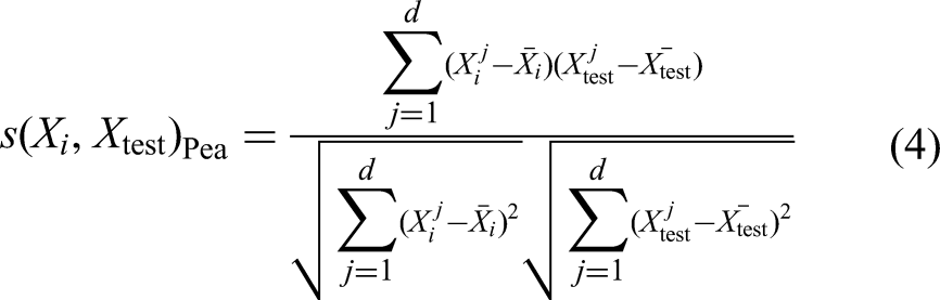
In the above formula, $X_{i}$ represents the $i$ th sample of historical data, $X_{i}^{j}$ and $X_{test}^{j}$ represent the characteristics of the $j$ th dimension of the two samples. $d$ is the dimension quantity of each sample. In addition to the Euclidean distance, Manhattan distance, cosine similarity, and Pearson correlation coefficient mentioned above, $K$ similarity measurement methods such as KNN nearest neighbour, Chebyshev distance, Lance–Williams distance, and Jaccard correlation coefficient are also used. Taking the hot rolling scenario as an example, the sample characteristics cover composition, production process parameters, and so on. A variety of distance measures are used to evaluate the proximity of samples in numerical characteristics, and similarity measures are used to measure the consistency of parameter adjustment patterns. For distance measurement, select the sample with the shortest distance from the sample to be tested. Taking Euclidean distance as an example, the formula for selecting samples is as follows:

S e t_{Euc} = {X_{i} | i \in {argmin}_{i \in {1, 2, \dots n}}^{m_{1}} d (X_{i}, X_{test})_{Euc}}

(5)

For similarity measurement, the sample with the highest similarity to the sample to be tested is selected. Taking cosine similarity as an example, the formula for selecting samples is as follows:

S e t_{Cos} = {X_{i} | i \in {argmax}_{i \in {1, 2, \dots n}}^{m_{1}} s (X_{i}, X_{test})_{Cos}}

(6)

By this method, we construct $K$ similar sample sets ${S e t_{Euc}, S e t_{Man}, S e t_{Cos}, S e t_{Pea} \dots}$ , and there are $m_{1}$ samples in each set. These sets reflect the similarity of the samples to be tested in different dimensions.

Integrating target similarity stage

In the process of steel key indicator measurement, measurement errors occasionally lead to significant deviations between readings and their true values. Meanwhile, even if certain historical samples exhibit high similarity in the feature space, unobserved characteristics with significant differences may still result in large deviations in measurement outcomes. In addition, for test samples that may possess abnormal indicators, it is necessary to select samples with boundary indicator values from the historical data to construct a similar sample set. This helps to identify potential high risks associated with the current sample.

Traditional JITL methods, which only rely on the similarity comparison between sample features, are not enough to effectively deal with the above complex situations. In order to solve this problem, the idea of target similarity is integrated to further compare the similarity of samples on the indicator. Specifically, first, build a pseudo-label prediction model³¹ based on all historical data. Here, the multiple linear regression model³² is used to give the sample to be tested a pseudo-label. Although relatively simple, the linear base model is deliberately chosen to strictly satisfy the millisecond-level inference latency constraints of legacy industrial control systems and edge computing devices.³³ The formula is as follows:

\begin{aligned} \begin{matrix} Y_{pseudo} & = f (X_{test}) = β_{0} + β_{1} X_{test}^{1} + β_{2} X_{test}^{2} \\ + β_{3} X_{test}^{3} + \dots + β_{n} X_{test}^{n} + ε \end{matrix} \end{aligned}

(7)

where

β_{0}

is the constant term,

β_{1}

β_{n}

are the corresponding coefficients of

1

n

dimensions of the sample,

ε

is the residual between the predicted value and the real value, and

Y_{pseudo}

is the predicted value given by the pseudo-label prediction model. The prediction model is trained through the historical data, and then the possible indicator values of the samples to be tested are predicted. It is used to select some samples from the

K

similar sample sets that are most likely to be similar to the indicator value of samples to be tested, and further optimise the selection of similar sample sets, to improve the prediction effect of the local model. Taking the first similar sample set

S e t_{Euc}

as an example, the formula of the selection process is as follows:

S e t_{Euc, tar} = {X_{i} | i \in {argmin}_{i \in S e t_{Euc}}^{m_{2}} | Y_{i} - Y_{pseudo} |}

(8)

By this method, we reconstruct $K$ similar sample sets ${S e t_{Euc, tar}, S e t_{Man, tar}, S e t_{Cos, tar}, S e t_{Pea, tar} \dots}$ , and there are $m_{2}$ samples in each set, where $m_{2} < m_{1}$ .

EL stage

In the field of EL, the bagging method focuses on improving the robustness of prediction, while the boosting method focuses on improving the accuracy of prediction. In view of the dual requirements of accuracy and robustness in the prediction of key indicators of steel process flow, the stacking method, which combines the advantages of the two methods, is selected in this study. The specific implementation steps are as follows:

Based on $K$ similar sample sets, $K$ different indicator prediction models are trained independently:

\begin{matrix} {S e t_{Euc, tar}, S e t_{Man, tar}, S e t_{Cos, tar}, S e t_{Pea, tar} \dots} \\ ==> \\ {f_{Euc}, f_{Man}, f_{Cos}, f_{Pea} \dots} \end{matrix}

(9)

The $K$ similar sample sets are merged to form an extended similar sample set;

\begin{matrix} S e t_{merge} = ⋃ S e t, \\ S e t \in {S e t_{Euc, tar}, S e t_{Man, tar}, S e t_{Cos, tar} \dots} \end{matrix}

(10)

The $K$ models trained in step (i) are used to predict the extended set of similar samples, and the $K$ groups of prediction results of the first layer are obtained:

P_{Euc} = {f_{Euc} (X_{i}) | X_{i} \in S e t_{merge}}

(11)

F = {P_{Euc}, P_{Man}, P_{Cos}, P_{Pea} \dots}

(12)

Taking $K$ groups of prediction results $F$ as input, the second layer model is trained, and the final prediction output is generated:

m o d e l = t r a i n (F, {Y_{i} | Y_{i} \in S e t_{merge}})

(13)

In this process, the $K$ models in the first layer capture different aspects of the prediction rules, while the second layer model is responsible for integrating these rules to achieve better prediction results. Through this two-stage model stacking, high-precision and high robustness prediction of key indicators of the steel process flow can be achieved.

Industrial deployment and practical application

To deploy the TS-EL-JITL framework in real-world steelmaking, an offline-training and online-inference paradigm is adopted. During the initial offline phase, historical process data specific to targeted production scenarios are continuously collected directly from the production line to construct a reliable sample pool. The pseudo-label model is then pre-trained to meet the strict millisecond-level latency constraints of legacy industrial control systems. Online, upon receiving a new sample, the system executes multi-dimensional similarity calculations. Following the target similarity mechanisms, the local stacking ensemble dynamically generates the final prediction. Furthermore, to maintain long-term adaptability to continuous condition deviations (e.g. equipment degradation), the historical database is periodically updated via a sliding window mechanism, ensuring system evolution without disrupting production.

Experimental design and result analysis

Experimental set-up and configurations

Experimental data and pre-processing

Data pre-processing

The original data feature dimension is often high, and there is also significant correlation between features. Therefore, pre-processing the data, eliminating redundant information, and retaining the main information of the data are of great significance to improve the data quality and better train the model.

The raw dataset first undergoes systematic data cleaning. Illegal sensor readings identified from an industrial perspective are converted to nulls and subsequently imputed using mean filling. Next, the Density-Based Outliers (DB_outliers) algorithm^34,35 is applied to detect and eliminate extreme anomalies while preserving genuine operating condition deviations. Following data cleaning, a comprehensive feature selection process is executed to reduce dimensionality and avoid ill-conditioned matrices during local modelling.^36,37 This process comprises three steps: (1) low variance screening to remove stagnant variables; (2) collinearity processing via Pearson correlation to exclude highly redundant features; and (3) low contribution processing using tree-based importance evaluation to retain only the critical target-related parameters. This streamlined sub-set ensures both accuracy and computational efficiency for the subsequent JITL modelling.

Dataset

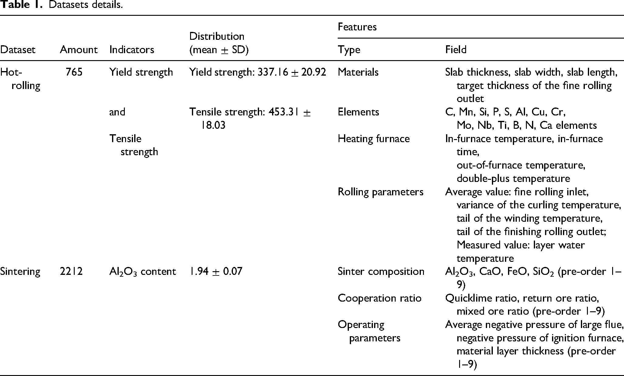
To comprehensively evaluate the proposed framework, we utilise two industrial datasets collected from typical steel manufacturing scenarios: the hot-rolling process and the sintering process. The feature variables in both datasets are directly acquired from the sensor networks of their corresponding production lines, encompassing material properties, chemical compositions, and various thermal-mechanical operating parameters. Detailed statistics of the two datasets, including sample amounts, target indicators with their distributions (mean $\pm$ SD), and specific feature categories, are summarised in Table 1. Furthermore, it is worth noting from an industrial application perspective that, while the raw datasets do not include discrete categorical variables explicitly labelling operational failures or pre- and post-maintenance schedules, they inherently capture these physical realities. Specifically, the continuous sensor readings (e.g. roll forces, motor currents, and negative pressures) and control parameters intrinsically reflect equipment degradation, manual parameter adjustments, and transitioning states over time. The gradual drifts and sudden shifts in these continuous variables constitute the very ‘dynamic operating condition deviations’ that our proposed TS-EL-JITL framework is fundamentally designed to address.

Table 1.

Datasets details.

Dataset	Amount	Indicators	Distribution(mean ± SD)	Features
Dataset	Amount	Indicators	Distribution(mean ± SD)	Type	Field
Hot-rolling	765	Yield strength	Yield strength: 337.16 ± 20.92	Materials	Slab thickness, slab width, slab length, target thickness of the fine rolling outlet
		and	Tensile strength: 453.31 ± 18.03	Elements	C, Mn, Si, P, S, Al, Cu, Cr,Mo, Nb, Ti, B, N, Ca elements
		Tensile strength		Heating furnace	In-furnace temperature, in-furnace time,out-of-furnace temperature,double-plus temperature
				Rolling parameters	Average value: fine rolling inlet,variance of the curling temperature,tail of the winding temperature,tail of the finishing rolling outlet;Measured value: layer water temperature
Sintering	2212	Al₂O₃ content	1.94 ± 0.07	Sinter composition	Al₂O₃, CaO, FeO, SiO₂ (pre-order 1–9)
				Cooperation ratio	Quicklime ratio, return ore ratio,mixed ore ratio (pre-order 1–9)
				Operating parameters	Average negative pressure of large flue,negative pressure of ignition furnace,material layer thickness (pre-order 1–9)

Experiments and baselines

Experimental set-up

In order to comprehensively evaluate the performance of the prediction model of key indicators of steel process flow adapting to the dynamic changes of operating conditions, three experiments were set up to verify the performances of three dimensions: global prediction ability, boundary conditions prediction ability, and operating condition deviation adaptability.

The first is the comparative experiment of the global prediction ability of the model. The dataset was divided into a training set and a test set according to time sequence, and the overall prediction performance of each model on the same test set was compared.

The second is the comparative experiment of boundary conditions prediction ability. The dataset was divided into training set and test set according to time sequence, and the prediction performance of each model on boundary samples (the top and bottom 25% quantiles) within the same test set was compared.

The third is the comparative experiment of operating condition deviation adaptability. The dataset is divided into training set and test set according to time sequence, and then the test set is divided into three test sections to observe the accuracy and robustness of the prediction results of the model in different test sections.

Hyper-parameter settings

The number of base models ( $K$ ) in the ensemble is not an arbitrarily tuned parameter, but is structurally determined by the number of distinct multi-dimensional similarity metrics employed in the JITL stage (e.g. Euclidean, Manhattan, cosine, Pearson). For the neighbourhood parameters, $m_{1}$ (initial sample pool size) and $m_{2}$ (optimised target-similarity pool size), their optimal values are highly dataset-dependent. In this study, they were determined through an empirical grid-search strategy based on an offline validation set. Specifically, $m_{1}$ is selected to be large enough to capture a statistically significant local feature space but small enough to exclude irrelevant historical states. Subsequently, $m_{2}$ ( $m_{2} < m_{1}$ ) is strictly fine-tuned to hone in on the precise target space, effectively balancing local modelling accuracy and the risk of overfitting.

Baseline models for comparison

blackTo comprehensively evaluate the TS-EL-JITL framework, six representative data-driven models were selected as baselines:

ML³²: a fundamental global parametric model establishing a single linear mapping across the entire historical dataset.

XGB³⁸: a powerful tree-based ensemble algorithm, representing a strong baseline for global non-linear static modelling.

LightGBM³⁹: a highly efficient, state-of-the-art gradient boosting framework utilising tree-based learning algorithms. It serves as a cutting-edge global non-linear baseline renowned for its fast inference speed and dominant performance on industrial tabular data.

HLRFR³: a global hybrid baseline combining linear and non-linear modelling for dynamic steelmaking processes, effectively contrasting with our local dynamic approach under condition deviations.

JITL²⁵: a conventional dynamic local model widely applied in current industrial soft sensing, selecting historical samples based solely on feature–space distances. It serves as a direct ablation baseline to validate our ensemble stacking and target-similarity mechanisms.

TabPFN⁴⁰: a cutting-edge tabular foundation model based on transformer architectures. It is included as a highly advanced deep learning baseline to evaluate the prediction accuracy of our proposed model.

Evaluation metrics

For the global prediction and boundary conditions prediction experiments, the commonly used evaluation metrics of regression tasks such as $R^{2}$ , hit rate, and mean absolute percentage error (MAPE) are used, including: $k %$ hit rate, which counts the proportion of the predicted value in the range of $k %$ above and below the real label value in all test samples. The larger the value, the better the prediction effect. The $k$ is usually 5 and 6. The calculation formula is:

k %_{hit_rate} = \frac{\sum_{i = 1}^{N} I (y_{i} (1 - k %) < \hat{y_{i}} < y_{i} (1 + k %))}{N}

(14)

where $N$ is the total number of test samples, $y_{i}$ is the real value of the $i$ th test sample, $\hat{y_{i}}$ is the predicted value of the $i$ th test sample, and $I ()$ is the indicating function, which is $1$ when the conditions are met, and $0$ if not.

For the comparative experiment of operating condition deviation adaptability, the above evaluation metrics are calculated for three test sections to measure the prediction accuracy. On this basis, the mean value and range of these indexes are calculated to further measure the robustness of the prediction results of the model in different test sections.

Comparative experiment of global prediction ability

In this experiment, the first 80% of the dataset is used as the training set, and the remaining 20% is used as the test set. In order to ensure the fairness of model comparison and objectively show model performance, linear regression is used as the base model for all models, including a traditional machine learning model (ML), JITL, and TS-EL-JITL. For the hot rolling scenario, the yield strength and tensile strength are predicted, and for the sintering scenario, the Al₂O₃ sinter composition is predicted. The prediction results are shown in Table 2. The bold result in each row is the best among the compared models for each evaluation metric.

Table 2.

Comparison experiment of global predictive ability (%).

Dataset	Indicator	Metric	ML	XGB	LightGBM	HLRFR	JITL	TabPFN	TS-EL-JITL
Hot-rolling	Yield strength	6% hit rate	72.38	74.29	77.90	79.05	80.00	80.19	85.71
		$R^{2}$	0.64	0.57	0.63	0.62	0.65	0.65	0.71
		MAPE	4.18	4.58	4.15	4.07	4.00	4.06	3.60
	Tensile strength	6% hit rate	97.14	94.29	95.24	96.19	98.10	98.11	99.05
		$R^{2}$	0.45	0.38	0.47	0.45	0.49	0.52	0.53
		MAPE	2.31	2.38	2.22	2.29	2.18	2.12	2.11
Sintering	Al $_{2}$ O $_{3}$	5% hit rate	93.94	88.01	92.58	90.05	94.21	92.82	95.87
		$R^{2}$	0.17	0.04	0.18	0.18	0.18	0.19	0.19
		MAPE	2.76	2.97	2.75	2.74	2.73	2.71	2.71

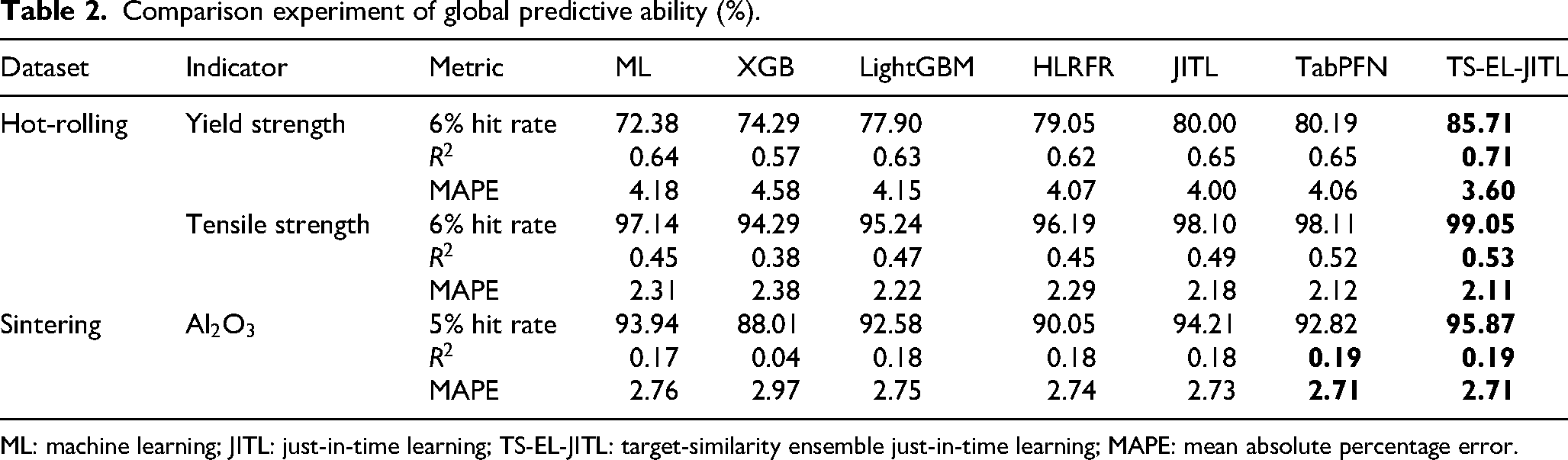
ML: machine learning; JITL: just-in-time learning; TS-EL-JITL: target-similarity ensemble just-in-time learning; MAPE: mean absolute percentage error.

As shown in Table 2, among the traditional global models, the state-of-the-art tree ensemble, LightGBM, notably outperforms standard ML and XGB, demonstrating strong non-linear fitting capabilities. Furthermore, the cutting-edge tabular foundation model, TabPFN, exhibits remarkable performance, even matching the best $R^{2}$ (0.19) and MAPE (2.71) in the sintering Al $_{2}$ O $_{3}$ prediction. However, despite their strong general regression abilities, these global modelling paradigms inherently struggle to adapt to the dynamic operating condition deviations and local data shifts prevalent in real-world metallurgical processes. This limitation becomes highly evident in the hot-rolling yield strength prediction, where TabPFN’s hit rate (80.19%) falls significantly behind our proposed method (85.71%). In contrast, models incorporating dynamic or local mechanisms show distinct advantages in this scenario. The hybrid global model HLRFR and the conventional JITL consistently outperform the static global baselines, confirming that local modelling is crucial for mitigating operating condition deviation. Finally, TS-EL-JITL achieves the best overall predictive performance across all indicators. This superiority is deeply rooted in its architectural design: while standard JITL selects samples solely based on feature–space distances (which can be misleading under severe sensor noise), TS-EL-JITL uniquely introduces a target-similarity mechanism to precisely constrain the local sample space. Coupled with an ensemble stacking strategy, it effectively absorbs the epistemic uncertainty of local pseudo-labels and suppresses prediction variance, thereby maintaining superior accuracy and robustness even under dynamic industrial environments.

Comparative experiment of boundary conditions prediction ability

In the iron and steel industry, the accurate prediction of boundary indicators is of great significance for timely early warning of boundary samples and the mitigation of production risks. For example, in the hot rolling scenario, boundary values of mechanical properties usually indicate high risk, requiring special attention. However, due to the long-tailed distribution of industrial data, this constitutes a challenging imbalanced regression problem where traditional global models often fail.⁴¹ In order to explore the performance of the model proposed in this study on the boundary values prediction task, the test sample set comprising label values beyond the central 50% range (specifically, those in the top 25% and bottom 25% tail distributions) was selected as the boundary values evaluation set to make statistics on the prediction effect. The results are shown in Table 3.

Table 3.

Prediction performance of boundary samples (%).

Indicator	Metric	ML	XGB	LightGBM	HLRFR	JITL	TabPFN	TS-EL-JITL
Yield strength	6% hit rate	49.02	56.86	64.71	66.67	70.59	64.71	76.47
	$R^{2}$	0.66	0.62	0.65	0.70	0.71	0.70	0.74
	MAPE	6.16	6.12	6.02	4.90	5.36	5.49	4.74
Tensile strength	6% hit rate	94.12	88.24	94.12	94.12	96.08	96.08	98.04
	$R^{2}$	0.57	0.45	0.62	0.58	0.59	0.63	0.63
	MAPE	2.87	3.26	2.71	2.75	2.75	2.70	2.68

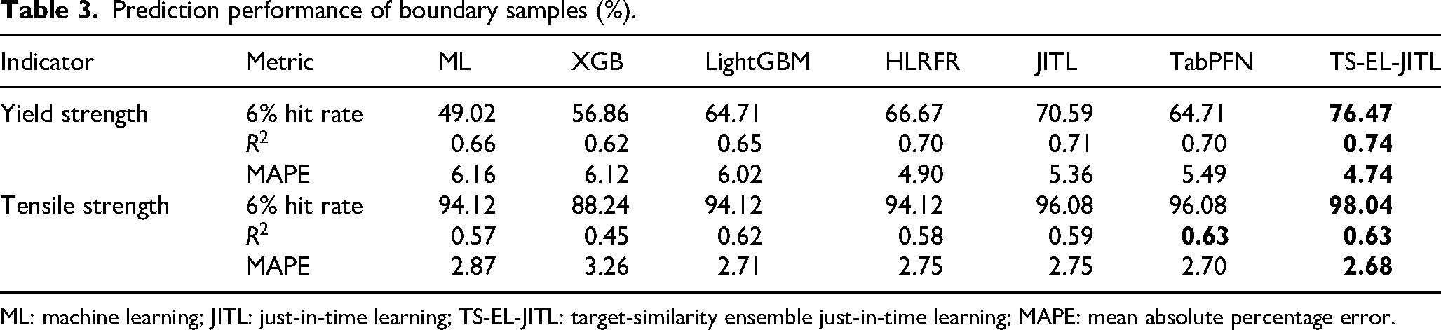
ML: machine learning; JITL: just-in-time learning; TS-EL-JITL: target-similarity ensemble just-in-time learning; MAPE: mean absolute percentage error.

Table 3 presents the predictive performance on boundary samples (top and bottom 25% quantiles). Predicting these long-tailed boundary values is a challenging imbalanced regression problem in metallurgical processes. Consequently, global models like LightGBM and TabPFN experience significant performance degradation (e.g. stagnating at a 64.71% hit rate for yield strength). This occurs because their global optimisation objectives inherently tend to over-smooth rare boundary values to fit the majority of normal samples. Conversely, localised strategies like JITL demonstrate better resilience (70.59% hit rate) but remain limited by relying solely on feature–space distances. Our proposed TS-EL-JITL successfully overcomes this, achieving an outstanding hit rate of 76.47% for yield strength (a 56% relative improvement over traditional ML) and 98.04% for tensile strength. By explicitly integrating the target similarity mechanism, TS-EL-JITL enables the algorithm to retrieve historical samples with matching boundary target behaviours. Furthermore, the ensemble stacking framework effectively mitigates the high variance and overfitting risks associated with modelling rare events. These results prove our method’s superiority in providing reliable early warnings for high-risk boundary conditions.

In order to further intuitively display the prediction performance of boundary values, the predicted values and real values of boundary samples from ML and TS-EL-JITL are compared, and the results are shown in Figure 2.

Figure 2.

Comparison chart of predicted value and real value. The shaded areas indicate the prediction deviation, highlighting the improved fitting accuracy of TS-EL-JITL at boundary values. TS-EL-JITL: target-similarity ensemble just-in-time learning.

As shown in Figure 2, from ML to TS-EL-JITL, the degree of fitting between the predicted results and the real values is significantly improved in the details of boundary low values (the shaded area is significantly smaller). In ML, where the fitting degree is not ideal, TS-EL-JITL has higher accuracy in both trend and numerical aspects. It is proven that TS-EL-JITL can significantly improve the prediction accuracy for boundary values and can more accurately predict high-risk situations.

To isolate the specific contribution of the target similarity module, an ablation experiment was conducted comparing TS-EL-JITL with EL-JITL (which excludes the target similarity mechanism). As shown in Figure 3, removing this module causes a notable performance decline across all metrics; for instance, the 6% hit rate drops from 76.47% to approximately 68.6%. This gap highlights that in complex industrial environments, feature–space similarity alone can be misleading when similar inputs yield divergent outputs, a phenomenon known as feature–target decoupling. By integrating target similarity, the model effectively constrains the local sample pool to those truly representative of the boundary target regime. This validates the module’s critical role in enhancing predictive accuracy and providing reliable early warnings for high risk.

Figure 3.

Performance comparison of TS-EL-JITL and EL-JITL in boundary values. The results are based on a deterministic evaluation of the fixed test set. TS-EL-JITL: target-similarity ensemble just-in-time learning; EL-JITL: ensemble just-in-time learning.

Visual analysis of sample space shrinkage

To intuitively demonstrate how the proposed target similarity mechanism mitigates feature–target decoupling, a Three-dimensional (3D) visualisation experiment of the sample selection process was conducted. We selected a representative boundary test sample from the hot-rolling dataset with a true yield strength of 285 MPa. The historical sample pool was projected into a 3D space, where the $X$ and $Y$ axes represent the principal latent feature dimensions (obtained via principal component analysis), and the $Z$ axis represents the actual target indicator. We then compared the local neighbourhood sets retrieved by the standard distance-based JITL and our TS-EL-JITL framework.

As illustrated in Figure 4, standard JITL initially selects a broad neighbourhood of 320 candidates (light blue dots) based solely on feature–space proximity. However, due to inherent measurement noise and unobserved industrial disturbances, these feature-similar samples exhibit severe divergence in the target domain, with many drifting towards the normal operational distribution. In contrast, by imposing the target similarity constraint, TS-EL-JITL effectively shrinks this candidate space. It filters out the ‘feature-similar but target-divergent’ false neighbours, retaining a highly refined sub-set of exactly 100 core samples (dark blue triangles) that tightly cluster around the 285 MPa boundary target. This visualisation explicitly proves that TS-EL-JITL successfully extracts a high-density, target-consistent sub-set from the noisy feature-similar domain, thereby fundamentally reducing pseudo-label uncertainty for boundary values prediction.

Figure 4.

Three-dimensional visualisation of sample space shrinkage via target similarity.

Comparative experiment on adaptability of operating condition deviation

In this study, the population stability index (PSI) was used to evaluate the operating condition deviation in the production process. PSI is an index widely used in the field of financial risk control. In recent years, it has also been introduced into the industrial scene to evaluate the product quality of the production line and the stability of the production process control. It is of great significance to improve the product quality and the control ability of the production line. The lower the PSI value, the more stable the production process. Specifically, the PSI value between 0 and 0.1 indicates that the production process has no change or changes very little, the PSI value between 0.1 and 0.25 indicates that the production process is slightly unstable, and when the PSI value exceeds 0.25, it indicates that the characteristics of the production process show great instability. The application of PSI can effectively monitor and evaluate the stability of the production process, and provide a scientific basis for timely adjustment and optimisation of production. The PSI was calculated for key production parameters to quantify their distribution shifts over time, with the results illustrated in Figure 5. It can be observed from the figure that the PSI values of almost all important production process parameters are significantly higher than 0.25 (red scatters), which indicates that the operating condition deviation phenomenon is very serious with the passage of time.

Figure 5.

PSI values of various production process parameters. The highly scattered distribution in the upper region (PSI > 0.25) explicitly demonstrates the severity of the operating condition deviation. PSI: population stability index.

To intuitively illustrate this dynamic deviation, the dataset was simply divided into four consecutive segments in chronological order to analyse the distribution of key features over time. As shown in Figure 6, the boxplots reveal that the statistical behaviours of these representative features (such as medians and data ranges) fluctuate significantly across the four segments. This visual evidence, consistent with the PSI results, intuitively confirms that operating condition drift continuously occurs within the dataset as time progresses.

Figure 6.

Time-segmented distribution of key features, illustrating the operating condition deviation.

In order to evaluate the impact of this model on the prediction performance of the target value when dealing with the dynamic deviation of operating conditions, the datasets are sorted in chronological order, and the training set and test set are divided accordingly: specifically, the first 70% of the dataset is used as the training set, the next 10% (i.e. 70% to 80% of the parts) is used as the first test set, the next 10% (i.e. 80% to 90% of the parts) is used as the second test set, and the last 10% (i.e. 90% to 100% of the parts) is used as the third test set. Based on this division, experiments on different models are carried out on the overall test set and three segmented test sets.

In the hot rolling quality prediction, the 6% hit rate and $R^{2}$ performance were evaluated in three different test stages for yield strength and tensile strength respectively. In the prediction of sintering composition, we evaluated the performance of 5% hit rate and $R^{2}$ in the same three test stages for Al₂O₃ content. Through the statistical analysis of the highest prediction performance, the lowest prediction performance, and the prediction mean value of each model in the three test stages, the adaptability and robustness of the model in dealing with the dynamic deviation of operating conditions are evaluated. The results are shown in Figure 7.

Figure 7.

Adaptability experiment of operating condition deviation. The shaded bands represent the fluctuation range (deviation) between maximum and minimum prediction performances across different chronological segments; a narrower band indicates higher robustness against condition deviation.

The results show that TS-EL-JITL achieves the best adaptation effect in the case of operating condition deviation. In the three test sections, the maximum prediction effect of the research model is better than that of the comparison model, and the prediction mean and minimum prediction effect are also the best in almost all cases, indicating that it can still maintain high prediction accuracy when dealing with the deviation of operating conditions. In addition, it can be observed that in the two experiments of hot rolling yield strength 6% hit rate and hot rolling tensile strength $R^{2}$ fraction, the model in this study significantly reduced the difference between the maximum and minimum prediction performances of the three test sections from 12.25 and 0.27 in ML to 5.06 and 0.09, greatly improving the prediction robustness.

To sum up, the experiment proves that TS-EL-JITL has strong adaptability in the case of dynamic deviation of operating conditions, which not only has advantages in prediction effect, but also has strong robustness. The superior performance of TS-EL-JITL under deviations can be heavily attributed to the variance-reduction property of the ensemble stacking mechanism. In real-world steel manufacturing, measurement noise and pseudo-label uncertainty are inevitable. While individual pseudo-labels or local models may suffer from this epistemic uncertainty, our approach of aggregating predictions across multi-dimensional similarity metrics inherently acts as a structural filter. This aligns with recent findings in advanced metallurgical modelling, where combining domain-knowledge integrated methods or ensemble frameworks significantly buffers the system against high-dimensional industrial noise and sensor anomalies.^12,42,43 By cross-validating the target similarity through multiple base learners, the final stacked output smooths out individual prediction spikes, thereby stabilising the indicator forecasting even when the underlying data drifts.

Conclusions

By integrating a target-similarity mechanism with EL-JITL, this study proposes the TS-EL-JITL framework to effectively overcome the feature–target decoupling problem in steel manufacturing.

Quantitatively, the framework delivers a maximum overall accuracy improvement of 18%. More meaningfully, for high-risk boundary samples, it achieves a 56% relative improvement in hit rate over traditional global baselines, providing reliable early warnings for industrial anomalies and effectively preventing the over-smoothing of critical production shifts.

The model demonstrates exceptional robustness against dynamic condition deviations. It successfully compresses the prediction accuracy fluctuation range across varying chronological segments from over 12% down to approximately 5%, ensuring highly stable performance in shifting industrial environments.

Future research will focus on cross-plant validation and fine-tuning advanced tabular foundation models (e.g. TabPFN) to capture deeper multi-indicator correlations, while strictly maintaining the millisecond-level inference latency required by legacy control systems.

Footnotes

ORCID iDs

Jinghan Zhang

Jia Wang

Bing Tang

Funding

The authors received no financial support for the research, authorship, and/or publication of this article.

Declaration of conflicting interests

The authors declared no potential conflicts of interest with respect to the research, authorship, and/or publication of this article.

Appendix

References

Jiang

Zhao

, et al. A joint model for hot-rolled strip quality in advance prediction. Ironmak Steelmak 2023; 50: 1224–1233.

Song

Qing

Xiaojie

, et al. Synthetically predicting the quality index of sinter using machine learning model. Ironmak Steelmak 2020; 47: 828–836.

de Matos

da Silva

Peixoto

JJM

, et al. A hybrid approach using multiple linear regression and random forest regression to predict molten steel temperature in a continuous casting tundish. Ironmak Steelmak 2023; 50: 1659–1667.

Shi

Tang

Chu

. Process metallurgy and data-driven prediction and feedback of blast furnace heat indicators. Int J Miner Metall Mater 2024; 31: 1228–1240.

Fan

, et al. Intelligent prediction and soft-sensing of comprehensive production indicators for iron ore sintering: a review. Comput Ind 2025; 165: 104215.

Diez-Olivan

Del Ser

Galar

, et al. Data fusion machine learning for industrial prognosis: trends and perspectives towards Industry 4.0. Inform Fusion 2019; 50: 92–111.

Xie

Suvarna

, et al. Online prediction of mechanical properties of hot rolled steel plate using machine learning. Mater Des 2021; 197: 109201.

Kwak

Kim

Ding

, et al. Machine learning prediction of the mechanical properties of

γ

-tial alloys produced using random forest regression model. J Mater Res Technol 2022; 18: 520–530.

Chen

Zeng

Yao

, et al. Flow-stress model of 300m steel for multi-pass compression. Metals 2020; 10: 438.

10.

Xiong

Yang

Guan

, et al. Combination of plasma acoustic emission signal and laser-induced breakdown spectroscopy for accurate classification of steel. Anal Chim Acta 2025; 1336: 343496.

11.

Chen

Zhang

Liu

, et al. A flow stress model of 300m steel for isothermal tension. Materials 2021; 14: 252.

12.

Shen

Wang

Wei

, et al. Physical metallurgy-guided machine learning and artificial intelligent design of ultrahigh-strength stainless steel. Acta Mater 2019; 179: 201–214.

13.

Huang

Jia

Shen

, et al. Deformation behavior and tensile properties of layered bis austenitic steel. JOM 2026; 1–12.

14.

Peng

Xie

Xia

, et al. Investigation of process and properties of Cu–Mn–Al alloy cladding deposited on 27SiMn steel via cold metal transfer. Crystals 2025; 15: 858.

15.

Yang

Sun

. Dynamic time features expanding and extracting method for prediction model of sintering process quality index. IEEE Trans Ind Inform 2021; 18: 1737–1745.

16.

, et al. A novel thermal error compensation framework towards precision manufacturing: integrating digital twin technology and edge server deployment. J Intell Manufactur 2026; : 1–39.

17.

Wang

Tao

Zhang

, et al. Spatial spiral tube multi-roller bending: accurate axial prediction utilizing AWPSO–FECAM–LSTM framework. Expert Syst Appl 2025; 128960.

18.

San Martín

Wang

, et al. A review of the thermal stability of metastable austenite in steels: martensite formation. J Mater Sci Technol 2021; 91: 200–214.

19.

Zhang

Zhao

. Slow-feature-analysis-based batch process monitoring with comprehensive interpretation of operation condition deviation and dynamic anomaly. IEEE Trans Ind Electron 2018; 66: 3773–3783.

20.

Widmer

Kubat

. Learning in the presence of concept drift and hidden contexts. Mach Learn 1996; 23: 69–101.

21.

Stenman

. Model on demand: Algorithms, analysis and applications. Linköping: Department of Electrical Engineering, Linköping University, 1999.

22.

Bontempi

Birattari

Bersini

. Local learning for iterated time series prediction. In ICML. pp. 32–38.

23.

Yang

. Rethinking the value of just-in-time learning in the era of industrial big data. IEEE Trans Ind Inform 2021; 18: 976–985.

24.

Dong

Cao

, et al. A survey on ensemble learning. Front Comput Sci 2020; 14: 241–258.

25.

Sheng

Qian

Song

, et al. A review of just-in-time learning-based soft sensor in industrial process. Can J Chem Eng 2024; 102: 1884–1898.

26.

Guo

Liu

Huang

. Just-in-time framework for robust soft sensing based on robust variational autoencoder. J Process Control 2024; 143: 103325.

27.

Shao

Song

. Bayesian just-in-time learning and its application to industrial soft sensing. IEEE Trans Ind Inform 2019; 16: 2787–2798.

28.

Dong

Tian

Peng

. Local multi-model integrated soft sensor based on just-in-time learning for mechanical properties of hot strip mill process. J Iron Steel Res Int 2021; 28: 830–841.

29.

Song

Cao

Liu

, et al. A local-model integration approach to the transition state prediction of continuous annealing processes. IEEE Trans Ind Inform 2025; 21: 743–751. DOI: 10.1109/TII.2024.3459050.

30.

Cao

, et al. Soft-sensing of burn-through point based on weighted kernel just-in-time learning and fuzzy broad-learning system in sintering process. IEEE Trans Ind Inform 2024; 20: 7316–7324.

31.

Wang

Yin

Zhou

, et al. A semisupervised just-in-time learning framework based on local label propagation and its application to industrial virtual sensing. IEEE Sens J 2023; 23: 24983–24992.

32.

Uyanık

Güler

. A study on multiple linear regression analysis. Procedia-Soc Behav Sci 2013; 106: 234–240.

33.

Heydari

Mahmoud

. Tiny machine learning on-device inference: a survey of applications, challenges, and future directions. Sensors 2025; 25: 3191.

34.

Jin

Liu

, et al. Varying-scale HCA-DBSCAN-based anomaly detection method for multi-dimensional energy data in steel industry. Inf Sci (NY) 2023; 647: 119479.

35.

. Evaluating the performance of SVM, isolation forest, and DBSCAN for anomaly detection. ITM Web Conf 2025; 70: 04012.

36.

Theng

Bhoyar

. Feature selection techniques for machine learning: a survey of more than two decades of research. Knowledge Inform Syst 2024; 66: 1575–1637.

37.

Iranzad

Liu

. A review of random forest-based feature selection methods for data science education and applications. Int J Data Sci Anal 2025; 20: 197–211.

38.

Chen

Guestrin

. XGBoost: a scalable tree boosting system. In Proceedings of the 22nd ACM SIGKDD international conference on knowledge discovery and data mining. pp. 785–794.

39.

Jin

Dogani

, et al. Enhancing LightGBM for industrial fault warning: an innovative hybrid algorithm. Processes 2024; 12: 221.

40.

Hollmann

Müller

Purucker

, et al. Accurate predictions on small data with a tabular foundation model. Nature 2025; 637: 319–326.

41.

Chen

Yang

, et al. A survey on imbalanced learning: latest research, applications and future directions. Artif Intell Rev 2024; 57: 137.

42.

Liu

Huang

, et al. A semisupervised soft-sensor of just-in-time learning with structure entropy clustering and applications for industrial processes monitoring. IEEE Trans Artif Intell 2022; 4: 722–733.

43.

Wang

Liu

, et al. Diameter-adjustable mandrel for thin-wall tube bending and its domain knowledge-integrated optimization design framework. Eng Appl Artif Intell 2025; 139: 109634.