Reconstructing the pattern of the Bara Shigri Glacier fluctuation since the end of the Little Ice Age,Chandra valley,north-western Himalaya

Abstract

The pattern of glacial records since the end of the Little Ice Age (LIA) are essential for evaluating glacier fluctuations and their link to post-LIA climate change. Although recession of the Himalayan glaciers is well-documented in this period, debate continues as to the magnitude and accuracy of estimated recession rates. This study presents a reconstruction of the pattern of fluctuations at the Bara Shigri Glacier in the Himachal Himalaya during the termination of the LIA (∼1850). A multi-data integrative analysis (MDIA) technique consisting of repeat terrestrial photographs, historical archives and reports, geomorphological evidence and maps, and high to medium spatial resolution satellite images (Corona, Hexagon, Landsat and WorldView-2) was used with supplemented by extensive field validation. The results indicate that during the early part of the 19th century the terminus of Bara Shigri Glacier was at ∼3900 m asl. Following this, there was a continuous recession with a total retreat of 2898 ± 50 m, which corresponds to a frontal areal loss of 4 ± 1 km² in the last 151 years (1863–2014). Compared to this, during the last half century (1965–2014), the glacierised area was reduced by 1.1 ± 0.02 km² with a concomitant terminus retreat of 1100 ± 32 m. The early 19th century advance is ascribed to a combination of cooling during this period, glacier topographical characteristics and contributions from steep-fronted avalanching tributaries. The late 19th century recession can be attributed to an overall increase in the temperature with a corresponding decrease in precipitation in the north-western Himalaya. Results are at variance with earlier, larger estimates of the frontal area loss for the Bara Shigri Glacier using either Survey of India (SoI) topographic maps or coarse spatial resolution satellite images (e.g. Landsat MSS) as historical datasets, and demonstrate the utility of mixed method approaches including higher-resolution satellite imagery for accurate estimation of glacier behaviour in this region.

Keywords

Little Ice Age (LIA)multi-data integrative analysis (MDIA)glacier change repeat terrestrial photographs geomorphological evidence remote sensing

I Introduction

The pattern of glacial records since the end of the Little Ice Age (LIA) are essential for evaluating glacier fluctuations and their link to post-LIA climate change. The term LIA was first coined by François E. Matthes (1939) to a glacial re-advance in Sierra Nevada, California, subsequent to the early/mid-Holocene hypsithermal. The LIA is a globally documented cooling event that began around the 13th or 14th century and culminated between the mid-16th and mid-19th centuries (Grove, 2004; Mann, 2002). Although the cause of LIA glaciation is not fully understood, climatologists contend that reduced solar output, changes in atmospheric circulation as a result of a reversal of the North Atlantic Oscillation and explosive volcanism could have decreased the global temperature (Crowley, 2000; Eddy, 1976; Mann et al., 2005). During the LIA, glaciers advanced in many mountainous regions worldwide. However, the timing and magnitude of LIA glacier advances vary across the world including in the Himalayan region (Bradley and Jonest, 1993; Grove 1988, 2004; Lowell, 2000; Mann et al., 1999; Owen and Dortch, 2014; Xu and Yi, 2014). In the Himalayan region, there is unequivocal evidence indicating that the LIA glaciation extended a few hundred metres below the present glacier snout positions (Ali et al., 2013; Barnard et al., 2004; Bisht et al., 2015; Dortch et al., 2013; Owen and Dortch, 2014; Sati et al., 2014; Sharma and Owen, 1996). Moreover, there are extensive permafrost features relating to this period. For instance, rock glaciers across the Himalaya indicate widespread ice retreat during the late Holocene, and likely more since the LIA at the turn of last century (Owen and England, 1998). However, compared to this, studies pertaining to the nature of deglaciation following the LIA are virtually non-existent, despite their importance in understanding the role of natural versus anthropogenic contributions to climate change and the ongoing debate on the impact of rising global temperatures on mountain glaciers (IPCC, 2007, 2013).

Historical records of individual glacier mapping in the Himalayan region date back to the early 1800s (e.g. Auden, 1937; Cotter and Brown, 1907; Finsterwalder, 1935; Finsterwalder and Pillewizer, 1937; Godwin-Austen, 1864; Hodgson, 1822; Longstaff, 1910; Mason, 1914, 1927a, 1927b, 1928; Mumm, 1909; Strachey, 1847; Visser, 1926, 1934; Workman, 1906). One of the early comprehensive studies pertaining to the historical glacier fluctuations since the early and mid-19th century was undertaken by Mayewski and Jeschke (1979). Based on their observations of 112 glaciers in the Hindukush-Karakoram-Himalaya (HKH) region, they inferred that the Himalayan glaciers have experienced a retreating trend since the mid-19th century, with some evidence of stable/advance phases during the second half of the early 20th century. Besides, recent studies suggest that many Himalayan glaciers showed enhanced recession over the most recent four decades (IPCC, 2007; Kulkarni et al., 2007). Hence, there seems to be little doubt that Himalayan glaciers have receded since the termination of LIA. However, what is debatable, particularly in the period since the availability of high-resolution remote sensing data (1960s–70s), is whether estimated rates of recession are accurate or overestimated. This debate occurs because earlier studies used either Survey of India (SoI) or coarse resolution satellite images (e.g. Landsat MSS) as historical datasets with limited field validations (Bhambri and Bolch, 2009; Chand and Sharma, 2015a, 2016).

Historical archives, repeated terrestrial photographs, old topographical/surveyed maps and published reports by earlier researchers and Geological Survey of India (GSI) provide an opportunity to reconstruct the history of Himalayan glaciers since the early 19th century. Typically, repeat photography (old and recent photographs) is a useful tool to document and reconstruct the changes of glacier terminus positions (Kamp et al., 2013; Webb, 2007). This method has been widely employed since the late 19th century in the European Alps (Zängl and Hamberger, 2004); Iceland (Hannesdóttir et al., 2014); Glacier National Park, Montana’s Rocky Mountains in the United States (http://nrmsc.usgs.gov/repeatphoto/overview.htm); the tropical mountains of Africa and South America (Hastenrath, 2008); the Turgen Mountains, Mongolian Altai (Kamp et al., 2013); and in the Himalaya, for example in the Khumbu Himal, Nepal (Byers, 2008), at the Raikot and Chungphare glaciers of Nanga Parbat in the western Himalaya (Nüsser and Schmidt, 2017; Schmidt and Nüsser, 2009) and recently at the Kolahoi Glacier in the Jammu and Kashmir (J&K) Himalaya (Rashid et al., 2017; Shukla et al., 2017). Thus, repeated photographs are used for glacier studies across the Himalayan region. Moreover, with the advent of remote sensing technology since the mid-20th century, it is now possible to monitor Himalayan glaciers from space (Paul et al., 2010; Racoviteanu et al., 2008; Raup et al., 2007).

The present study is undertaken on the Bara Shigri Glacier, which is known to be the largest glacier in the state of Himachal Pradesh, north-western Himalaya. The idea behind selecting this glacier was that it has the field-based observational records and archived repeat photographs, historical documents and published reports by explorers since the 1860s. In view of this, this glacier provides a rare opportunity to investigate the pattern and causes of deglaciation (glacier terminus and frontal area change) since the termination of LIA (post ∼1850). The specific objectives are: i) to reconstruct and quantify the changes in glacier terminus and the frontal area between 1863 and 2014; and ii) to analyse the possible causes of glacier recession such as temperature, precipitation (climatic) and non-climatic factors (e.g. glacier morphology, topography and debris cover).

II Regional and climate settings

Bara Shigri (32.17° N, 77.68° E) is a compound valley glacier, located in the Chandra valley of Himachal Himalaya, which lies to the north of the Pir-Panjal and the south of the Great Himalayan ranges (Figure 1). The glacier has an area of ∼126 km² with a length of ∼26 km. The dominantly south-east to north-west trending glacier headwall lies at an altitude of 6363 m asl, whereas the terminus is located at ∼3984 m asl. The snout of the glacier is well defined and is confined within a narrow U-shaped valley (Figure 1). The lower 25% of the ablation zone of the glacier is debris covered (Sangewar, 1995; Figure 1) and is riddled with transverse, longitudinal and marginal crevasses of a few metres to 200 m long, and with variable widths of up to 3 m (Sangewar, 1995). The average snowline altitude (SLA) computed from multi-temporal Landsat satellite images (2000–2014) lies at ∼5340 ± 30 m asl.

Figure 1.

(a) Map showing the location of the Bara Shigri Glacier in north-western Himalaya; (b) Bara Shigri Glacier and its tributary glaciers; (c) Temperature and rainfall trend of the nearest IMD station located at Tandi. The inset picture shows simplified topography–precipitation relationship from south to north swath of 20 km along the Pir-Panjal and Greater Himalayan range in the western Himalaya (Himachal Pradesh). RGI v4 Inventory (Arendt et al., 2014) for glacier boundaries except Bara Shigri Glacier in (b).

Climatically, the glacier lies in the transitional climatic zone between the cold, semi-arid, dry, temperate and sub-alpine zones (Rawat et al., 2009). The dominant influence of the Indian summer monsoon (ISM) is obstructed by the Pir-Panjal ranges in the south, whereas the Great Himalayan ranges in the north obstruct the direct influence of mid-latitude westerlies (Figure 1b). The rainfall data from the nearby Indian Meteorological Department (IMD) station at Tandi (∼3000 m asl; 32.55° N, 76.98° E), which is located ∼70 km from the glacier, suggests ISM contribution of ∼242 mm a^-1, whereas the winter precipitation which falls as snow is ∼466 mm a^-1. The annual average maximum temperature is ∼6.5°C with a maximum temperature of 23.3°C observed in August. The annual minimum temperature is –0.5°C with a lowest minimum temperature of –13°C recorded in January (Rawat et al., 2009). Moreover, based on automatic weather station data (4863 m asl; 1 October 2009 to 30 September 2013) at the Chhota Shigri Glacier, which adjoins the Bara Shigri Glacier, Azam et al. (2014) reported January (–15.8°C) and August (4.3°C) as the coldest and warmest months, respectively.

III Data sources and methods

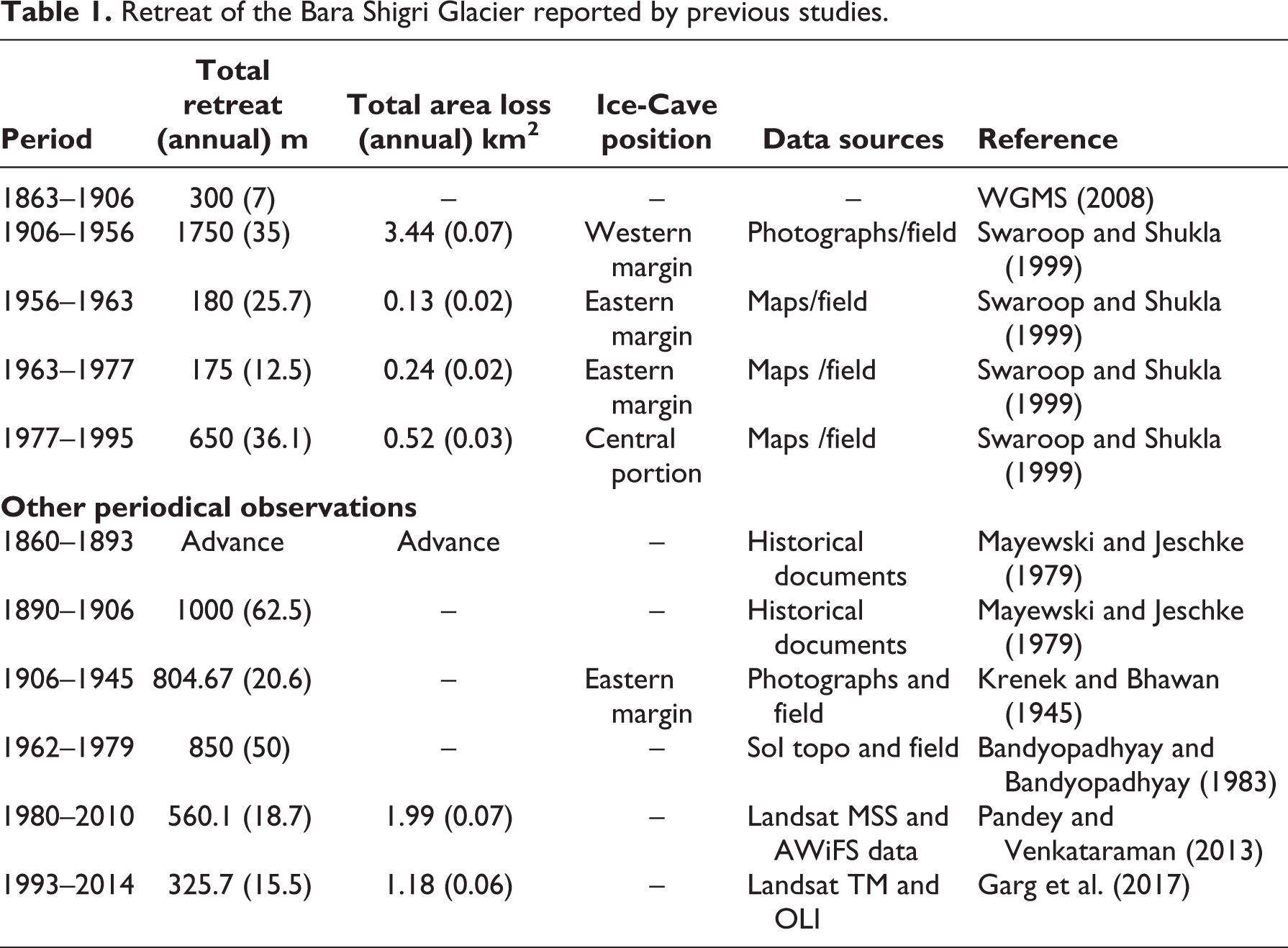
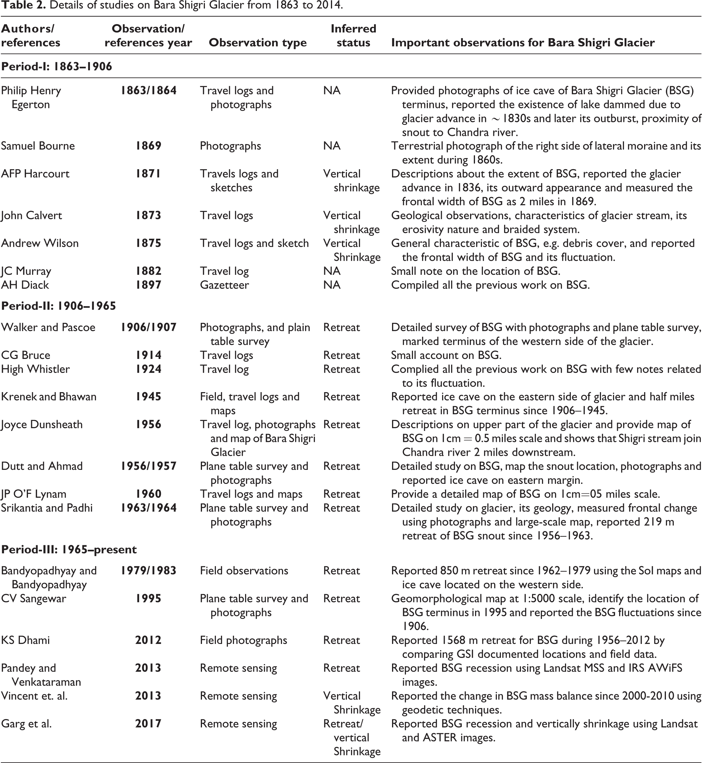
We used the repeated terrestrial photographs, available historical records and high to medium spatial resolution remote sensing images, supported by detailed geomorphological mapping, to assess glacier area changes. Unlike the majority of the Himalayan glaciers, the Bara Shigri Glacier has a long and relatively continuous research history. The earliest references to the Bara Shigri Glacier can be traced to the 1860s, a period that was supposedly the beginning of the LIA deglaciation (Grove, 2004; Xu and Yi, 2014). These include travel logs, historical archives, published reports and terrestrial photographs since the mid-19th century (∼1860s), with noted descriptions regarding the advance of the Bara Shigri Glacier during the fourth decade of early 19th century (∼1830s). Table 1 summarises the reported area/terminus change studies carried out by various researchers. The research history of the Bara Shigri Glacier, and inferences extracted from this, is summarised in Table 2. For clarity, the previous observations are grouped into three segments (1863–1906, 1906–1965 and 1965–2014) by taking consideration of used datasets and methods.

Table 1.

Retreat of the Bara Shigri Glacier reported by previous studies.

Period	Total retreat (annual) m	Total area loss (annual) km²	Ice-Cave position	Data sources	Reference
1863–1906	300 (7)	–	–	–	WGMS (2008)
1906–1956	1750 (35)	3.44 (0.07)	Western margin	Photographs/field	Swaroop and Shukla (1999)
1956–1963	180 (25.7)	0.13 (0.02)	Eastern margin	Maps/field	Swaroop and Shukla (1999)
1963–1977	175 (12.5)	0.24 (0.02)	Eastern margin	Maps /field	Swaroop and Shukla (1999)
1977–1995	650 (36.1)	0.52 (0.03)	Central portion	Maps /field	Swaroop and Shukla (1999)
Other periodical observations
1860–1893	Advance	Advance	–	Historical documents	Mayewski and Jeschke (1979)
1890–1906	1000 (62.5)	–	–	Historical documents	Mayewski and Jeschke (1979)
1906–1945	804.67 (20.6)	–	Eastern margin	Photographs and field	Krenek and Bhawan (1945)
1962–1979	850 (50)	–	–	SoI topo and field	Bandyopadhyay and Bandyopadhyay (1983)
1980–2010	560.1 (18.7)	1.99 (0.07)	–	Landsat MSS and AWiFS data	Pandey and Venkataraman (2013)
1993–2014	325.7 (15.5)	1.18 (0.06)	–	Landsat TM and OLI	Garg et al. (2017)

Table 2.

Details of studies on Bara Shigri Glacier from 1863 to 2014.

Authors/references	Observation/references year	Observation type	Inferred status	Important observations for Bara Shigri Glacier
Period-I: 1863–1906
Philip Henry Egerton	1863/1864	Travel logs and photographs	NA	Provided photographs of ice cave of Bara Shigri Glacier (BSG) terminus, reported the existence of lake dammed due to glacier advance in ∼1830s and later its outburst, proximity of snout to Chandra river.
Samuel Bourne	1869	Photographs	NA	Terrestrial photograph of the right side of lateral moraine and its extent during 1860s.
AFP Harcourt	1871	Travels logs and sketches	Vertical shrinkage	Descriptions about the extent of BSG, reported the glacier advance in 1836, its outward appearance and measured the frontal width of BSG as 2 miles in 1869.
John Calvert	1873	Travel logs	Vertical shrinkage	Geological observations, characteristics of glacier stream, its erosivity nature and braided system.
Andrew Wilson	1875	Travel logs and sketch	Vertical Shrinkage	General characteristic of BSG, e.g. debris cover, and reported the frontal width of BSG and its fluctuation.
JC Murray	1882	Travel log	NA	Small note on the location of BSG.
AH Diack	1897	Gazetteer	NA	Compiled all the previous work on BSG.
Period-II: 1906–1965
Walker and Pascoe	1906/1907	Photographs, and plain table survey	Retreat	Detailed survey of BSG with photographs and plane table survey, marked terminus of the western side of the glacier.
CG Bruce	1914	Travel logs	Retreat	Small account on BSG.
High Whistler	1924	Travel log	Retreat	Complied all the previous work on BSG with few notes related to its fluctuation.
Krenek and Bhawan	1945	Field, travel logs and maps	Retreat	Reported ice cave on the eastern side of glacier and half miles retreat in BSG terminus since 1906–1945.
Joyce Dunsheath	1956	Travel log, photographs and map of Bara Shigri Glacier	Retreat	Descriptions on upper part of the glacier and provide map of BSG on 1cm = 0.5 miles scale and shows that Shigri stream join Chandra river 2 miles downstream.
Dutt and Ahmad	1956/1957	Plane table survey and photographs	Retreat	Detailed study on BSG, map the snout location, photographs and reported ice cave on eastern margin.
JP O’F Lynam	1960	Travel logs and maps	Retreat	Provide a detailed map of BSG on 1cm=05 miles scale.
Srikantia and Padhi	1963/1964	Plane table survey and photographs	Retreat	Detailed study on glacier, its geology, measured frontal change using photographs and large-scale map, reported 219 m retreat of BSG snout since 1956–1963.
Period-III: 1965–present
Bandyopadhyay and Bandyopadhyay	1979/1983	Field observations	Retreat	Reported 850 m retreat since 1962–1979 using the SoI maps and ice cave located on the western side.
CV Sangewar	1995	Plane table survey and photographs	Retreat	Geomorphological map at 1:5000 scale, identify the location of BSG terminus in 1995 and reported the BSG fluctuations since 1906.
KS Dhami	2012	Field photographs	Retreat	Reported 1568 m retreat for BSG during 1956–2012 by comparing GSI documented locations and field data.
Pandey and Venkataraman	2013	Remote sensing	Retreat	Reported BSG recession using Landsat MSS and IRS AWiFS images.
Vincent et. al.	2013	Remote sensing	Vertical Shrinkage	Reported the change in BSG mass balance since 2000-2010 using geodetic techniques.
Garg et al.	2017	Remote sensing	Retreat/ vertical Shrinkage	Reported BSG recession and vertically shrinkage using Landsat and ASTER images.

3.1. Repeated photographs, historical archives and maps

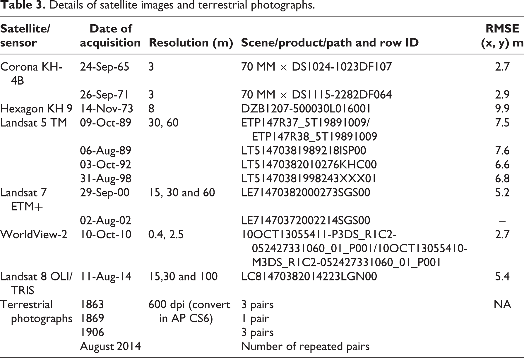
A number of repeated photographs, travel logs, historical archives, published reports and maps have been available since the mid-19th century (Table 3). For example, Egerton and Bourne took photographs of the terminus and lateral extent of the Bara Shigri Glacier in 1863 and 1869, respectively. Following this, GSI took numerous photographs of the Bara Shigri Glacier terminus during 1906, 1956, 1963 and 1995 (Table 2). In August 2014, we acquired repeated photographs at almost the same camera angle with the same field of view to infer frontal changes of the glacier. Repeated photographs were acquired using a simple parallax assessment of ridgeline intersections, perspective alignments and locations of similar foreground features (Kamp et al., 2013). Several reference points on previous photographs, e.g. moraines, rocky scarps, visible bedrock characteristics and foreground peaks, were precisely identified in the field and further taken into account during repeated photography in 2014. Additional information on the historical terminus and extent of the Bara Shigri Glacier has also been inferred from numerous historical documents preserved since the 1860s (details are given in Table 2).

Table 3.

Details of satellite images and terrestrial photographs.

Satellite/ sensor	Date of acquisition	Resolution (m)	Scene/product/path and row ID	RMSE (x, y) m
Corona KH-4B	24-Sep-65	3	70 MM × DS1024-1023DF107	2.7
	26-Sep-71	3	70 MM × DS1115-2282DF064	2.9
Hexagon KH 9	14-Nov-73	8	DZB1207-500030L016001	9.9
Landsat 5 TM	09-Oct-89	30, 60	ETP147R37_5T19891009/ETP147R38_5T19891009	7.5
	06-Aug-89		LT51470381989218ISP00	7.6
	03-Oct-92		LT51470382010276KHC00	6.6
	31-Aug-98		LT51470381998243XXX01	6.8
Landsat 7 ETM+	29-Sep-00	15, 30 and 60	LE71470382000273SGS00	5.2
	02-Aug-02	15, 30 and 60	LE71470372002214SGS00	–
WorldView-2	10-Oct-10	0.4, 2.5	10OCT13055411-P3DS_R1C2-052427331060_01_P001/10OCT13055410-M3DS_R1C2-052427331060_01_P001	2.7
Landsat 8 OLI/TRIS	11-Aug-14	15,30 and 100	LC81470382014223LGN00	5.4
Terrestrial photographs	1863	600 dpi (convert in AP CS6)	3 pairs	NA
	1869		1 pair
	1906		3 pairs
	August 2014		Number of repeated pairs

3.2. Satellite images

The availability of high to medium spatial resolution remote sensing data since the 1960s assists in monitoring the historical extent of the Bara Shigri Glacier with an acceptable accuracy of ± 2-5% (Paul et al., 2002, 2013; Table 3). The early US military reconnaissance Corona satellite (1965 and 1971) and Hexagon satellite data (1973) with high spatial resolution (3 m and 8 m) were used to widen the time span for monitoring the historic extent of the glacier back to the 1960s–70s. These datasets provide relatively consistent results when compared to the SoI topographic maps and coarse resolution satellite datasets (Chand and Sharma, 2015a; Table 3). Landsat satellite data of multi-spatial, spectral and temporal resolutions are used for mapping glacier area, terminus and debris-covered changes since the 1990s (Table 3). This includes imagery obtained from the Thematic Mapper (TM; 1989, 1992, 1998), Enhanced Thematic Mapper (ETM+; 2000, 2002) and Operational Land Imager (OLI; 2014) sensors. High-resolution (∼0.5 and 2.5 m) WorldView-2 (2010) images with limited swath (∼16.4 km at nadir) allowed us to identify and map the glacier terminus with high accuracy for the recent period (2010). A small gap, ∼10% of the total width of the Bara Shigri Glacier terminus (on the frontal right side of the glacier), in the WorldView-2 (2010) data was covered by same satellite images acquired by Bing Maps (http://www.bing.com/maps). Most of the satellite images were selected for the end of the ablation period with minimum snow cover and cloud cover, and with a high solar position to avoid shadows (Paul and Svoboda, 2009; Table 4). The Corona, Hexagon and Landsat datasets were downloaded from the United States Geological Survey (USGS) webpage (http://earthexplorer.usgs.gov/), whereas WorldView-2 images were provided by DigitalGlobe (http://www.digitalglobe.com) under ‘WorldView-2 8-Band Challenge’. The ortho-rectified Landsat ETM+ PAN imagery (2002) was used as a base image for the image to image rectification of the other satellite data (i.e. the Landsat, Corona, Hexagon and WorldView-2 images). The Landsat ETM+ PAN image (2002) is processed in standard terrain correction (level L1 T) that incorporates a digital elevation model (DEM) and ground control points (GCPs) to produce a higher accuracy image in comparison to the non-ortho-rectified image. Accordingly, the Landsat TM images, which have a slight horizontal shift as compared to the base image of Landsat ETM+ 2002, were corrected using the projective transformation algorithm inbuilt in the AutoSync tool of Erdas Imagine 10 by incorporating ASTER GDEM V2. Additionally, the image to image rectification (e.g. spline adjustment) method of ESRI ArcGIS 10 was used for rectification of WorldView-2 and Corona/Hexagon images. Stable river junctions, peaks and road junctions were used to collect GCPs from the Landsat ETM+ PAN merged image (2002) and handheld non-differential global positioning system (GPS) during field work (2014). To assess positional accuracy, 14–23 common location points such as river and road junctions, peaks and rocky outcrops were identified in all rectified images and simultaneously in a reference image of Landsat ETM+ PAN (2002). The horizontal shifts between the reference image and corresponding rectified images of WorldView-2 (2010), Corona (1965), Corona (1971) and Hexagon (1973) were 2.7 m, 2.9 m, 2.8 m and 8.9 m, respectively. The ASTER GDEM V2 (∼30 m spatial resolution) from Japan Space Systems (http://gdem.ersdac.jspacesystems.or.jp/) was used as a reference DEM for the extraction of glacier topographic parameters. During the field expedition in August 2014, the Bara Shigri Glacier terminus and recessional/terminal moraines were mapped using a handheld non-differential GPS (Garmin GPSMAP 76Cx, ± 3 to 10 m) for the accessible areas, and a Bushnell handheld laser distance metre (LDM with an accuracy of ±1 m) for the inaccessible areas.

Table 4.

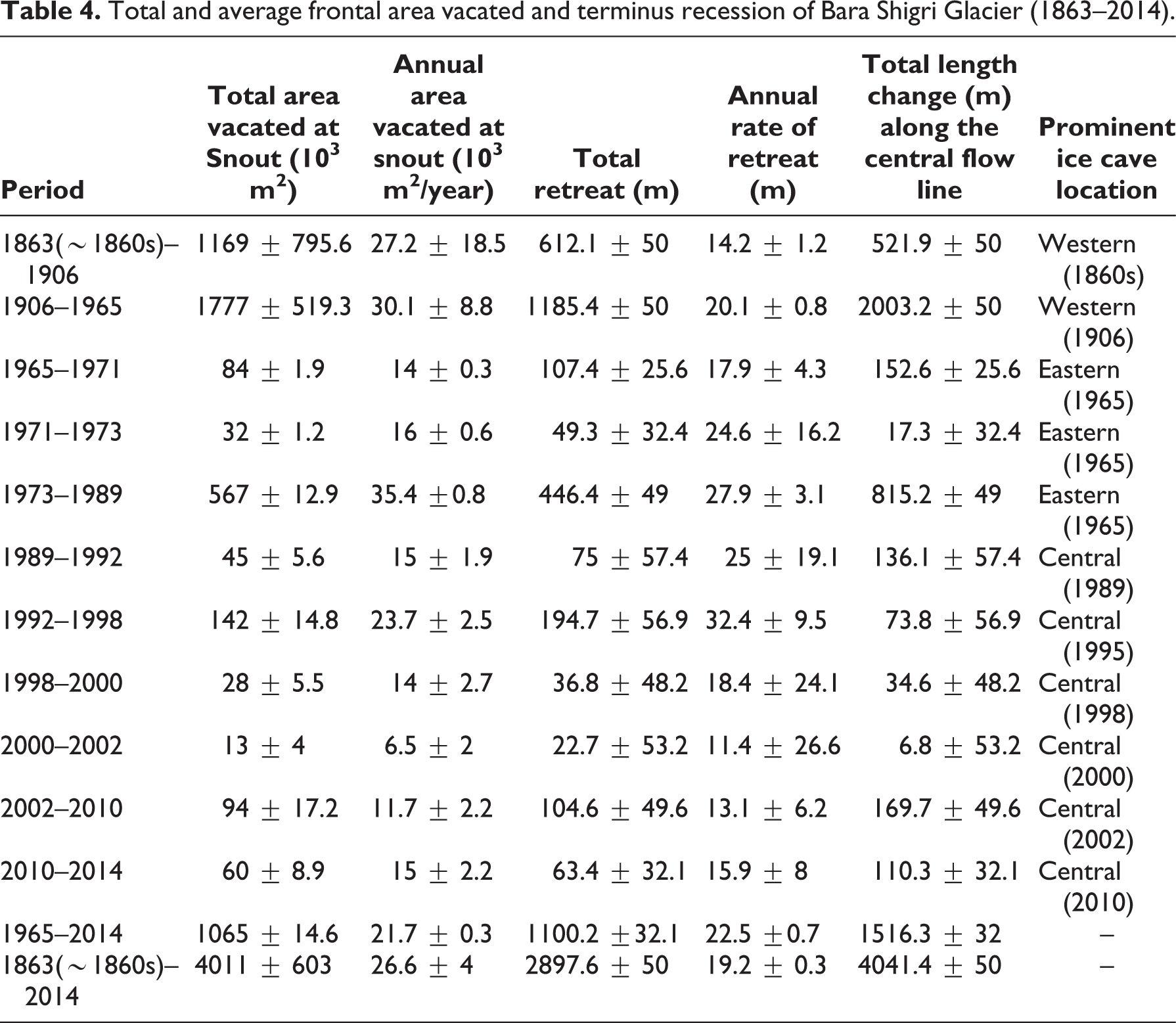
Total and average frontal area vacated and terminus recession of Bara Shigri Glacier (1863–2014).

Period	Total area vacated at Snout (10³ m²)	Annual area vacated at snout (10³ m²/year)	Total retreat (m)	Annual rate of retreat (m)	Total length change (m) along the central flow line	Prominent ice cave location
1863(∼1860s)–1906	1169 ± 795.6	27.2 ± 18.5	612.1 ± 50	14.2 ± 1.2	521.9 ± 50	Western (1860s)
1906–1965	1777 ± 519.3	30.1 ± 8.8	1185.4 ± 50	20.1 ± 0.8	2003.2 ± 50	Western (1906)
1965–1971	84 ± 1.9	14 ± 0.3	107.4 ± 25.6	17.9 ± 4.3	152.6 ± 25.6	Eastern (1965)
1971–1973	32 ± 1.2	16 ± 0.6	49.3 ± 32.4	24.6 ± 16.2	17.3 ± 32.4	Eastern (1965)
1973–1989	567 ± 12.9	35.4 ±0.8	446.4 ± 49	27.9 ± 3.1	815.2 ± 49	Eastern (1965)
1989–1992	45 ± 5.6	15 ± 1.9	75 ± 57.4	25 ± 19.1	136.1 ± 57.4	Central (1989)
1992–1998	142 ± 14.8	23.7 ± 2.5	194.7 ± 56.9	32.4 ± 9.5	73.8 ± 56.9	Central (1995)
1998–2000	28 ± 5.5	14 ± 2.7	36.8 ± 48.2	18.4 ± 24.1	34.6 ± 48.2	Central (1998)
2000–2002	13 ± 4	6.5 ± 2	22.7 ± 53.2	11.4 ± 26.6	6.8 ± 53.2	Central (2000)
2002–2010	94 ± 17.2	11.7 ± 2.2	104.6 ± 49.6	13.1 ± 6.2	169.7 ± 49.6	Central (2002)
2010–2014	60 ± 8.9	15 ± 2.2	63.4 ± 32.1	15.9 ± 8	110.3 ± 32.1	Central (2010)
1965–2014	1065 ± 14.6	21.7 ± 0.3	1100.2 ±32.1	22.5 ±0.7	1516.3 ± 32	–
1863(∼1860s)–2014	4011 ± 603	26.6 ± 4	2897.6 ± 50	19.2 ± 0.3	4041.4 ± 50	–

3.3. Climate data

For climate trends, we used the Climate Research Unit (CRU, 1×1 degree) monthly TS v.3.22 (1900−2010) and US National Center for Environmental Prediction/National Center for Atmospheric Research (NCEP/NCAR) monthly reanalysis data (at 700 hPa, i.e. ∼3100 m asl, 1948−2010) for the nearest grid of 32.5^o N, 77.5^o E, covering the period since 1900 and 1948, respectively. Reanalysis data are extensively used in recent climate studies, to extract glacier-climate parameters and to reconstruct the long-term glacier mass balance (Agrawal et al., 2014; Azam et al., 2014; Kumar et al., 2014; Schauwecker et al., 2015). However, considering that these data have inherent limitations in terms of accuracy and applicability in the high relief Himalayan region, we only used these datasets to understand the general trends and to make a comparison with previously reported climatic trends in north-western Himalaya extracted using climate proxies such as pollen, tree rings and ice cores. In addition, as mentioned earlier, precipitation data from the Tandi station (∼3000 m asl; 32.55° N, 76.98° E; Figure 1a) for the period 1975 to 2010 (35 years) are analysed to examine snowfall and rainfall trends. Monthly data were used to obtain average indices for annual and seasonal (December, January, February, March: DJFM; June, July, August: JJA) values of T_min and T_max temperature and precipitation. A widely used non-parametric Mann–Kendall test was used to determine any statistically significance trends (Bhambri et al., 2011).

3.4. The multi-data integrative analysis (MDIA) technique

The MDIA technique is used to reconstruct glacier terminus and boundary positions using a number of repeat photographs, geomorphological maps, field observations/mapping and high-resolution satellite images. This involves analysis of multiple datasets/layers that are pooled into one matrix to improve quality and accuracy of information extraction from multi-source datasets. Kamp et al. (2013) successfully applied this method to examine the glacier cover changes in the Turgen Mountains and Mongolian Altai. Accordingly, we used multi-layers/information derived from repeated photographs, field and remote sensing (using Corona and WorldView-2 images) mapping of LIA moraines and post-LIA deglaciated geomorphic features. All the acquired repeated photographs were processed in Adobe Photoshop (AP) CS-6 software for consistency in spatial resolution (600 dpi), geometry and overlapping, as described by Kamp et al. (2013). However, the method suggested by Kamp et al. (2013) was modified according to the objective of the present study. The information extracted from repeated photographs and high-resolution Corona and WorldView-2 satellite images include the past positions of the glacier terminus and lateral boundaries. The detailed geomorphological map on the scale of 1:1000 was prepared using a high spatial resolution WorldView-2 image (0.5 m), and further checked and validated in the field (Tobler, 1987; Figure 2). This map mainly depicted the landforms (e.g. lateral, recessional and hummocky moraines, flutes and paleochannels) moulded due to deglaciation since the end of LIA in order to reconstruct the glacier boundary (Loibl et al., 2014).

Figure 2.

Geomorphological map at 1:1000 scale (modified after Owen et. al., 1996, 2001) for the deglaciated area of the Bara Shigri Glacier along with reconstructed glacier extent for the period 1863/1869 (∼1860s) and 1906 (∼1900s).

The processed data and mapped layers were integrated into a geographical information system (GIS) to identify the terminus position and extent of the Bara Shigri Glacier in the 1860s and 1900s. For instance, blended hybrid photographs of the 1860s (1863 and 1869) and 2014 were created and overlaid in AP CS6 software to map and identify the glacier terminus and extent, as well as prominent landscape features of the 1860s (1863 and 1869) on 2014 photographs. Further, 3-D visualisation analysis was carried out by draping and overlaying the geomorphological layers, field reference points and GPS points/tracks and photo locations on high-resolution satellite images and the DEM in ArcScene 10. The draped and overlaid layers were rotated on multiple axes to locate and map the glacier terminus and glacier extent during the 1860s (1863 and 1869).

After confirming the locations of glacier terminus in the 1860s (1863 and 1869), the vectors files were drawn in the GIS for further change detection (Figure 3). The MDIA technique was repeated to identify and map the glacier terminus and its extent in 1906 (Figure 4). Additionally, the GSI report of 1907 provided detailed information and photograph references for the Bara Shigri Glacier terminus and extent, which helped to improve the mapping accuracy and reconstruction of 1906 glacier extent (Walker and Pascoe, 1907). All photographic stations I, II and III of Walker and Pascoe (1907) were plotted on the WorldView-2/Corona/Landsat images (draped on DEM) on the basis of information related to back bearing from the peaks A, B, C mentioned on photographs (1906) by Walker and Pascoe (1907). This was done using Google Virtual Compass applications on Google Earth images and then further validated and fixed during the 2014 (August) field survey with Silva compass, clinometer and handheld GPS.

Figure 3.

Reconstructed Bara Shigri Glacier extent and identification of its terminus in 1863 (∼1860s) using the repeated photographs of (a) 1863, (b) 1869 (∼1860s) and 2014 with a supplement of extensive field geomorphological observations.

Figure 4.

The Bara Shigri Glacier extent reconstruction based on repeated photographs of 1906 and 2014, supplemented with detailed geomorphological observations.

3.5. Glacier mapping and length change

The Bara Shigri Glacier has heterogenic surface characteristics, ranging from clean ice in the accumulation zone to extensive debris cover areas in the lower ablation zone. The clean ice area was mapped using a semi-automated band ratio method followed by a 3×3 median filter to eliminate isolated pixels (Frey et al., 2012; Paul et al., 2002). The lower debris-covered ablation zone could not be mapped using semi-automatic methods as the spectral signature scarcely differentiate debris-covered ice from the surrounding bare moraines. Therefore, we used manual digitisation to map the extent of debris-covered glacier areas from multi-spectral (Landsat TM/ETM+/OLI, WorldView-2) and panchromatic images, e.g. Corona (1965, 1971) and Hexagon (1973) (Bhambri et al., 2011; Paul and Svoboda, 2009). Additionally, signs of movement (identified based on overlays of multi-temporal images), emerging meltwater streams at the terminus, breaks in surface slope, spectral colour and texture differences, and the presence of ice walls were used to identify glacier terminus positions in the satellite images (e.g. Bhambri et al., 2013; Bolch et al., 2010b; Chand and Sharma, 2015b). The glacier terminus location for the year 2014 and earlier years were further validated in the field, using a handheld GPS and LDM, by mapping of the recessional moraines and relict melt streams (Hubbard and Glasser, 2005; Loibl et al., 2014). The change in glacier length was calculated by drawing parallel stripes at a 50-metre distance interval along the central flowline (Bhambri et al., 2012; Chand and Sharma, 2015b; Schmidt and Nüsser, 2009). Due to the irregular shaped glacier front, the recession rate varies; therefore, the glacier length change is calculated as the average length from the intersection of the stripes with the glacier outlines and referred as average length change (Chand and Sharma, 2015b). In addition, we estimated length change along the central flow line for comparison with average length change.

3.6. Mapping uncertainty

This study used repeat photographs, multi-temporal and multi-spatial satellite datasets. These datasets are subject to uncertainty, which propagates in the glacier area mapping and needs proper consideration to ascertain the accuracy of the results. Thus, the mapping uncertainty from satellite data is calculated on the basis of a buffer around the glacier margins, as suggested by Granshaw and Fountain (2006). Accordingly, the buffer size is chosen to be half of the pixel resolution of the satellite image used for mapping (Bolch et al., 2010a) and was set to 2.5 m, 7.5 m, 15 m and 10 m for the Corona/WorldView-2, Landsat 7 ETM+/ Landsat 8 OLI, Landsat TM and Hexagon images, respectively. The uncertainty associated with the derived glacier length changes is calculated (equation 1) using the approach suggested by Hall et al. (2003)

e = \sqrt{{(a 1)}^{2} + {(a 2)}^{2}} {+ E}_{reg},

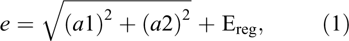
where a1 and a2 are the pixel resolution of image 1 and image 2, respectively, and E_reg is the registration error. Accordingly, the uncertainty calculated for individual images is given in Table 4. The glacial frontal area change uncertainty for satellite data was estimated by multiplication of the uncertainty of length with glacier mean width (Bhambri et al., 2012). The glacier average width is calculated by drawing parallel stripes at 50-metre intervals across the glacier boundary. The uncertainty in the positions of the glacier terminus in 1863 and 1906 was expected to be minimal (± 20 m) as it was validated rigorously in the field and clearly identified during MDIA. However, the uncertainties for the 1863 (∼1860s) and 1906 (∼1900s) averaged glacier termini (based on a 50 m parallel interval line strip method) and reconstructed glacier boundaries were expected to be higher since they were mainly based on interpolation from repeated photographs, geomorphological mapping and field evidence such as lateral and recessional moraines, positions of relict meltwater channels (paleochannels) and identification of deglaciated geomorphological features based on high-resolution satellite imagery (Corona and WorldView-2). The uncertainty in the averaged glacier terminus and reconstructed glacier boundary is typically within a 50 m buffer on both sides of the glacier terminus and the LIA deglaciated geomorphological features mapped in the field. Accordingly, the mapping uncertainty for calculated glacier averaged terminus in 1863 (∼1860s) and 1906 (∼1900s) were expected at 50 m. Moreover, the uncertainty for the reconstructed glacier boundaries in 1863 (∼1860s) and 1906 were calculated using the Granshaw and Fountain (2006) method, by taking a higher buffer of 50 m. Further, the area change uncertainty for 1863 (∼1860s) and 1906 (∼1900s) were estimated according to standard error propagation to be the root sum square of the uncertainty for the outlines mapped (Bhambri et al., 2013; Chand and Sharma, 2015a).

IV Results

4.1. Post-LIA glacier fluctuations

The Bara Shigri Glacier shows a pattern of continuous recession during the past 151 years (1863–2014). During this period, the average recession was estimated to be 2898 ± 50 m with an annual recession rate of 19.2 ± 0.3 m. The total area vacated by the glacier at its front from 1863 to 2014 is 4 ± 0.6 km² (0.03 ± 0.004 km² a^-1), which is ∼3.2% of the total glacier area (Table 4 and Figures 3 –6). The visual comparison of repeated photographs of 1863 and 1906, satellite images of 1965, recent repeated photographs of 2014 and field observations also suggest that the glacier has receded significantly (Figures 3 –5). However, the recession rate varied considerably in different observational time periods (1863–2014). To maintain consistency with previously reported glacier change and the availability of datasets, the 151 years time frame is separated into three periods, i.e. 1863–1906, 1906–1965 and 1965–2014, including the reported advance in ∼1830s (e.g. Egerton, 1864; Harcourt, 1871; Walker and Pascoe, 1907; Wilson, 1875).

Figure 5.

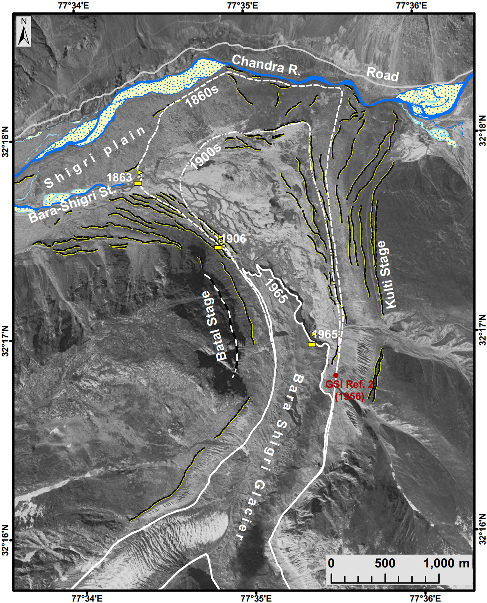
Reconstructed Bara Shigri Glacier boundary in 1863/1869 (∼1860s), 1906 (∼1900s) and 1965 on the high-resolution image of Corona (1965) with identified and marked terminus location (flag symbol with yellow colour) of the Bara Shigri Glacier in 1863, 1906 and 1965. GSI reference point of 1956 also marked with brown colour for reference. Morainic ridges represented the Batal and Kulti Stage as per Owen et al. (1996, 2001).

Figure 6.

Fluctuation of the Bara Shigri Glacier terminus between 1965 and 2014 with field photographs for 2014. Note the detached dead ice covered with debris as marked in the field (red colour with 40% transparent), otherwise difficult to identify from the coarse resolution satellite images, e.g. Landsat MSS.

Early 19th century–1860s

Repeated photographs, historical documents, GSI reports and most previous studies suggest that the terminus of the Bara Shigri Glacier rapidly advanced in the ∼1830s, with stagnation and slower recession in later decades (1850s–60s) (e.g. Egerton, 1864; Harcourt, 1871; Walker and Pascoe, 1907; Wilson, 1875). According to Egerton (1864), the advance of the Bara Shigri Glacier during the 1830s caused damming of the Chandra river. This is well represented by the existence of the ice-marginal moraine-dammed lake on the right flank of the glacier and is implicit by the extent of the Bara Shigri Glacier in the photographs of 1863 taken by Egerton and Bourne in 1869 (Figures 3 and 4). Stratigraphically, the advanced glacial ice that dammed the Chandra river can be assigned to the LIA ice-marginal moraines, corresponding to the Sonapani-II stage of Owen et al. (1996, 2001). Previous studies and repeated photographs suggest minimum frontal area change during the 1850s–60s (Egerton, 1864). For instance, Egerton (1864) reported that the glacier snout was close to the tributary of the Chandra river and there was diminutive space in between the channel of the river and the snout of the glacier (Figure 3). Besides, the photograph provided by Egerton (1864) from 1863 shows that a terminus/ice cave was located in the western central part of the glacier (Figures 3 and 5). In addition to this, the photograph provided by Bourne in 1869 shows the farthest right extent of a glacier lobe was on the northern side of the present snout, where the current Chandra river flows. However, the photograph (1869) does not show any lake or stagnant water upstream of the Bara Shigri outwash plain and the Chandra river flows continuously (Figure 3). This would imply that the glacier marginally receded in the later part of the 1850s–60s. In addition, Egerton (1864) reported that there was no contact of the ice terminus with the frontal part of the LIA moraine. Accordingly, we tend to suggest that during the 1860s the glacier terminus and ice mass was positioned at ∼3898 ± 15 m asl, in the present-day Bara Shigri outwash plain (Figures 3 and 5).

1863(∼1860s)–1906

The period from 1863 to the beginning of the 20th century, i.e. 1906, was marked by ice depletion and frontal area change at the Bara Shigri Glacier. During this period, the glacier shows signs of recession, confirmed by the sequence of repeated photographic evidence from the 1860s (1863 and 1869) and 1906 (Figures 3 and 4). Significant glacier mass loss was possibly due to down wasting, as indicated by supraglacial lakes observed by travellers and researchers during the early part of the 1870s (e.g. Harcourt, 1871; Wilson, 1875). In 1906, the Bara Shigri Glacier terminus was located on the western flank of the glacier tongue (∼3903 ± 15 m asl), which accords with the photograph taken by Walker and Pascoe (1907). During our detailed field mapping, we recognised moraine ridges and ground reference points, thus the reconstructed position of the glacier terminus suggests an average terminus retreat rate of 612 ± 50 m (14.2 ± 1.2 m a^-1), with a frontal surface area loss of 1.2 ± 0.8 km², corresponding to an annual rate of 0.03 ± 0.02 km². Interestingly, we found that compared to the western flank of the glacier, maximum area loss was observed in the centre and on the right flank (Figures 3, 4 and 5; Table 4).

1906 (∼1900s)–1965

Based on the GSI’s repeated photographs of 1906, 1956 and 1963, and the position of the recessional moraine ridges, it is clear that the lower frontal tongue of the Bara Shigri Glacier changed significantly from 1906 to 1965 (59 years) (Figures 4 and 5). Additionally, the Corona (1965) image shows this recession and shifting of the Bara Shigri Glacier’s terminus towards the eastern side of the tongue, at an altitude of ∼3906 ± 15 m asl with a total average retreat of 1185.4 ± 50 m (20.1 ± 0.8 m a^-1) (Figure 5). During this period, a loss 1.8 ± 0.52 km² in glacier area occurred at an annual rate of 0.03 ± 0.02 km² (Figure 5 and Table 4). These observations are in accordance with the GSI’s repeated photographs, maps and reports, suggesting a preferential shifting of the glacier towards the eastern flank. This shift can be ascribed to the influence of snow and ice avalanches from steep western slopes. Moreover, the uneven retreat of the glacier terminus (i.e. the difference between the western, central and eastern sectors) may be attributed to the differential radiance due to a shadow cast on the western side of the glacier by an adjoining ridge, maximum exposure to sunlight of the central and eastern part of the glacier, and varying thickness of supraglacial debris, which cumulatively prevent the western side of the glacier snout from melting (Figure 5). In addition, field-based observations of GSI during 1956–1963 revealed that the average retreat was minimised on the western flank (105 m), as compared to the eastern flank (180 m) (Srikantia and Padhi, 1964; Swaroop and Shukla, 1999).

1965–2014

The high to medium resolution satellite images of Corona (1965/1971), Hexagon (1973), Landsat (1989, 1992, 1998, 2000, 2002, 2014) and WorldView-2 (2010) supported by the recent field observation (August 2014) suggests that the Bara Shigri Glacier has experienced continual recession since 1965 (Figure 6 and Table 4). The average total recession of the Bara Shigri Glacier between 1965 and 2014 was estimated to be 1100.2 ± 32.1 m with an annual rate of 22.5 ± 0.7 m. The total frontal area vacated by the glacier for the period between 1965 and 2014 is 1.1 ± 0.01 km² with an annual rate of 0.02 ± 0.0003 km², which is approximately 0.9% of the total glacier area. During the year 1965, the active ice cave was prominent on the eastern margin of the glacier. This cave was also presented in 1956, as reported by Dutt and Ahmad (1957) and Dutt (1961). During 1965 to 1973, the average total recession of the glacier terminus was estimated to be 146.5 ± 32.3 m with total area loss of 0.12 ± 0.003 km². Whereas, the total area vacated by the glacier for the period between 1973 and 1989 was 0.6 ± 0.01 km² with average snout retreat of 446.4 ± 49 m. During this period, the position of the active ice cave changed from the eastern flank to the central part of the glacier. During 1989 to 2002, the total area vacated by the glacier was 0.2 ± 0.03 km² with an estimated average snout retreat of 273 ± 61.8 m. The ice cave position as observed in 1990 (central part) was found to be the same during 1995 (Sangewar, 1995). According to Sangewar (1995), the shifting of the ice cave is dependent on the network and gradient of the sub-glacial channels and feeding mechanism from the nearby steep slopes. During the past decade (2002−2014), the glacier has receded 150.3 ± 53.3 m, with an area loss of 0.15 ± 0.02 km². However, during the last four years (2010−2014), the glacier lost 0.06 ± 0.009 km² of its area with average annual recession rate of 15.9 ± 8 m, which can be considered as the present rate of frontal area loss and terminus retreat (Table 4). In 2014, the ice cave was recorded in the right eastern part of the glacier (Figure 6).

4.2. Temporal changes in climate

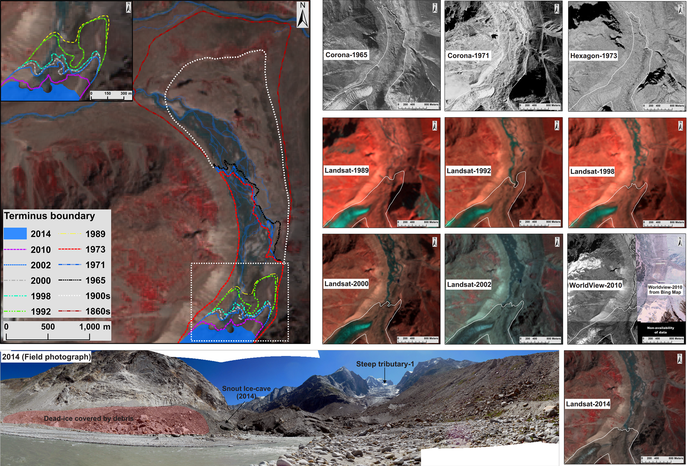
The annual average (T_avg), maximum (T_max) and minimum (T_min) temperature for the nearest grid point of CRU data show significant warming trends since 1900, with some cyclic drifts. Moreover, the dotted line in Figure 7 shows the five-year moving average, which gives a better representation of the temporal changes in temperature and precipitation. The annual T_avg (CRU) during 1900 to 1940 was found to be relatively low when compared to the T_avg during 1940 to 1970 (Figure 7c). Additionally, after the ∼1970s, T_avg shows a decreasing trend until the ∼1990s followed by an increasing trend (Figure 7c). However, the CRU gridded precipitation data shows significant decreasing trends in overall precipitation in this region and particularly after 1960, with some cyclic increasing trends of precipitation during 1900−1920 and 1940−1960 (Figure 7a). Also, the overall linear trend line for the annual average temperature and precipitation of NCEP/NCAR (at 700 hPa, i.e. ∼3100 m asl, 1948−2014) indicates an increasing and decreasing trend, respectively, during the last half century (1948–2014) (Figure 7e, f). In addition, the winter (DJF) T_avg shows a significant warming trend in comparison to annual T_avg and summer T_avg (Figure 7e). There is a significant decrease in annual precipitation between 1948 and 2014, due to a decrease in summer (JJA) and winter precipitation (DJFM) (Figure 7f). However, the Tandi IMD data shows an insignificant decreasing trend in annual snowfall as compared to the rainfall, which shows a slight increase during the same period (1975–2010) (Figure 7b, d). Overall, reanalysis datasets of CRU and NCEP/NCAR at century and half century time scales, respectively, show decreasing annual precipitation trends, whereas annual temperature shows an increasing trend, which is mainly noticeable during winter months. Moreover, the field-based Tandi data overall shows a decreasing and increasing trend in annual snowfall and rainfall, respectively, during the almost last four decades (1975–2010).

Figure 7.

Temperature and precipitation trends for the nearest grid (32.5^o N, –77.5 ^o E) of CRU ((a), (c): 1900–2013) and NCEP/NCAR ((e), (f): 1948–2014) and for Tandi IMD station ((e), (f):1975–2015). Note CRU and NCEP/NCAR is a reanalysis dataset and strictly used to capture the general regional climate trends.

V Discussion

5.1. Post-LIA glacier fluctuations

LIA moraines in the Himalaya are either sharply-crested or nested hummocky moraines, and are well preserved within a few hundred metres from the terminus of contemporary glaciers (Ali et al., 2013; Bisht et al., 2015; Dortch et al., 2013; Owen and Dortch, 2014). Recently, Xu and Yi (2014) collated the published radiocarbon, lichenometry and cosmogenic radionuclide (CRN) ages for LIA moraines from the Tibet Plateau (TP) and bordering area of the Himalaya, indicating two major phases of glacier advance during the LIA. According to them, the older advance occurred during late 14th century to 16th century AD, whereas the younger glacial advance was observed during the late 18th to early 19th centuries, which they attributed to temperature rather than the precipitation changes (Xu and Yi, 2014). The beginning of the 20th century is marked by the accelerated recession of LIA glaciers, which continues to present, however, with variations from one glacier to another (Bhambri and Bolch, 2009; Bolch et al., 2012; Mayewski and Jeschke, 1979; Figure 8). There seems to be a broad correspondence between the Bara Shigri Glacier and regional advancing and recessional trends observed during the younger phase of the LIA in Himalaya and the TP. We observed an advance of the Bara Shigri Glacier during the early 19th century followed by a recessional trend after the mid to late 19th century (∼1860s). Moreover, our observations indicate a slower average frontal recession and frontal area loss since 1863 (∼1860s) and during the last few decades, as compared to the previously reported estimates (e.g. Bandyopadhyay and Bandyopadhyay, 1983; Garg et al., 2017; Mayewski and Jeschke, 1979; Pandey and Venkataraman, 2013; Swaroop and Shukla, 1999). This can be attributed to differences in methodology and datasets used by earlier researchers. For instance, the present study suggests that the Bara Shigri Glacier retreated by 612.1 ± 50 m (14.2 ± 1.2 m a^-1) between 1863 (∼1860s) and 1906, whereas Mayewski and Jeschke (1979) reported that it retreated by 1000 m (62.5 m a^-1) during the 1890s to 1906. During 1906 to 1965, the present study suggests that the glacier reduced by 1185.4 ± 50 m (20.1 ± 0.8 m a^-1), which is much less than the recession of 1750 m (35 m a^-1) between 1906 and 1956 reported by the GSI (Swaroop and Shukla, 1999). However, it is consistent with the retreat, i.e. 2003.2 ± 50 m (34 ± 0.8 m a^-1), calculated along the central flow line during 1906 to 1965. Bandyopadhyay and Bandyopadhyay (1983), using the SoI topographic maps, reported 850 m (50 m a^-1) retreat for the terminus of the Bara Shigri Glacier during 1962 to 1979, which is higher than the estimate (at annual scale) from the present study (146.5 ± 32.21 m; 18.3 ± 4 m a^-1) and GSI (Sangewar, 1995) (175 m; 12.5 m a^-1) during 1965–1973 and 1963–1977, respectively. The higher retreat rate of Bandyopadhyay and Bandyopadhyay (1983) could be due to erroneous glacier outline reconstruction using SoI topographic maps (Bhambri and Bolch, 2009; Chand and Sharma, 2015a). Pandey and Venkataraman (2013) reported 560.1 m (18.7 m a^-1) retreat with a total loss of 1.9 km² (0.07 km² a^-1) for the Bara Shigri Glacier during 1980 to 2010 using the coarser resolution satellite data of Landsat MSS (1980) and IRS AWiFS (2010). Recently, Garg et al. (2017) reported 325.7 m (15.5 m a^-1) retreat with the total loss of 1.2 km² (0.06 km² a^-1) for the Bara Shigri Glacier during 1993 to 2014 using the Landsat TM (1993) and Landsat OLI (2014) images, which is similar to Pandey and Venkataraman (2013). The glacier terminus retreat rate reported by Pandey and Venkataraman (2013) is lower than our study (23.8 ± 0.9 m a^-1 during 1973 to 2010 and 19.2 ± 2.2 m a^-1 during 1992 to 2014); however, the total area loss is significantly higher than our estimate of 0.9 ± 0.01 km² during 1973 to 2010 and 0.34 ± 0.01 km² during 1992 to 2014 (as compared to Garg et al., 2017) based on higher to medium resolution Hexagon (1973), Landsat TM (1992), WorldView-2 (2010) and Landsat 8 OLI (2014) satellite data supplemented by field observations (2014). These differences can be attributed mainly to difficulties with identifying the limits of extensively debris covered glaciers when using coarse to medium resolution images of Landsat MSS and TM. This is particularly true when trying to differentiate the detached debris-covered dead ice part from the debris-covered ice of the main trunk, due to spectral homogeneity in the coarse and medium satellite images (Figure 6; Chand and Sharma, 2016). Thus, high to medium resolution satellite data of Corona, WorldView-2 and Landsat-8, with a supplement of field observation, provide more reliable results than those based on coarser resolution satellite datasets (Landsat MSS and IRS AWiFS). Our results, based on the average length from the intersection of the stripes with the glacier outlines, suggest 1100.2 ± 32.1 m recession of the Bara Shigri Glacier from 1965 to 2014, whereas recession of 1516.3 ± 32.1 m is observed along the central flow line. This suggests that averaging along the front is a more robust method and provides more reliable estimates, especially in the situation of a change in location of the ice caves, and can be one of the causes for discrepancy in retreat rates as compared to previous studies (Bhambri et al., 2012; Chand and Sharma, 2015b; Schmidt and Nüsser, 2009).

Figure 8.

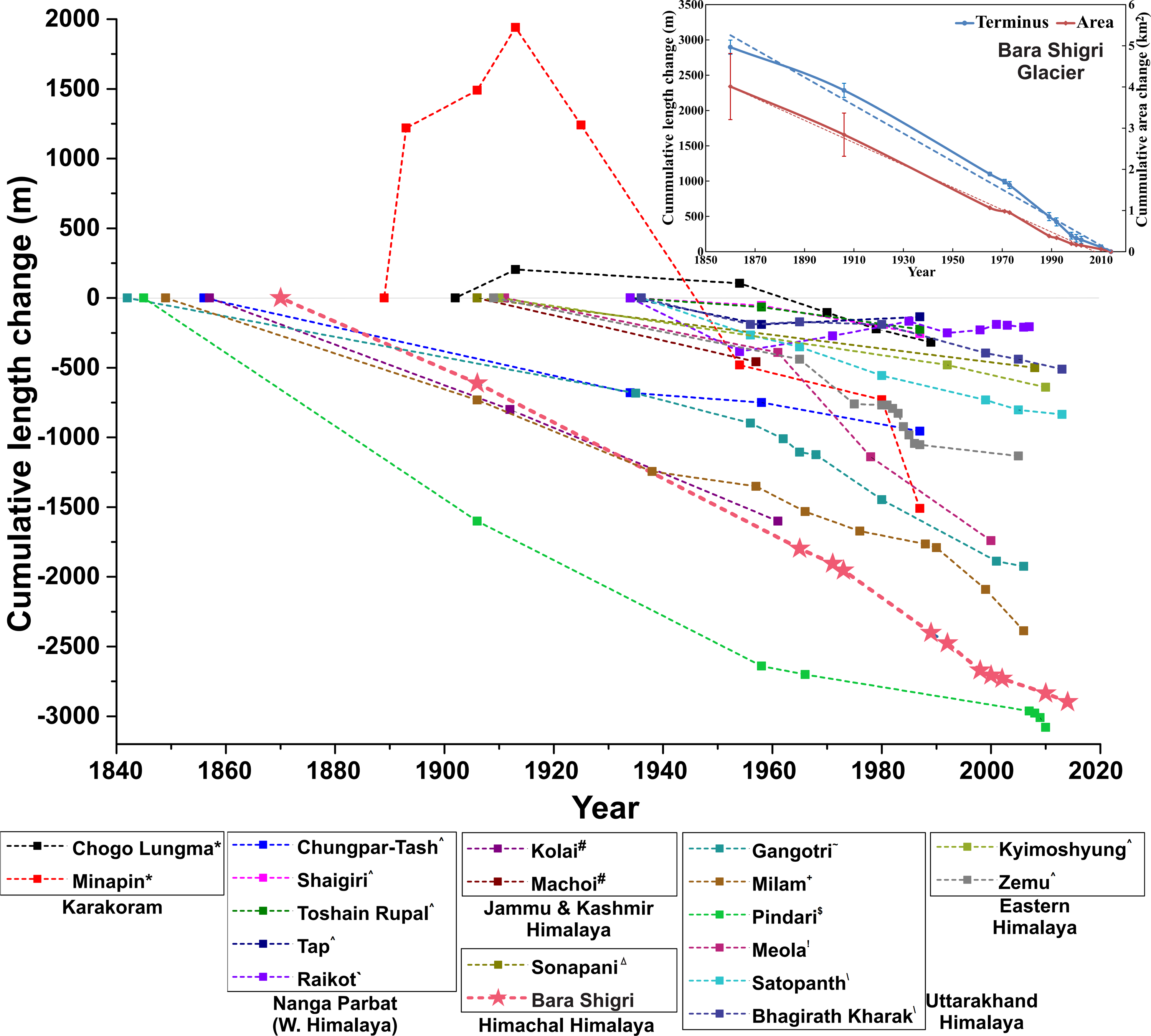
Long-term cumulative length changes of selected Karakoram Himalayan glaciers; the markers indicate the years of measurements. The inset picture shows a change in the Bara Shigri Glacier terminus and frontal area since 1863 (∼1860s) and the best-fit straight lines and associated errors bar are also shown. Symbols after glacier name are representing the reference, i.e. * (Hewitt, 2011), ^ (WGMS, 2008),` (Schmidt and Nüsser, 2009), ^# (Raina, 2009), ^Δ (Swaroop and Shukla, 1999), ^∼ (Bhambri and Bolch, 2009; Bhambri et al., 2012), ⁺ (GSI, 1997; Raj, 2011), ^$ (Bali et al., 2013), ^! (GSI, 2000), ^\ (Nainwal et al., 2016).

Recent studies indicate that the Himalayan glaciers are losing mass at rates similar to those observed elsewhere, with large variability from one glacier to another (Bolch et al., 2012). Long-term termini fluctuation records are limited and available for selected glaciers in the Himalayas and Trans-Himalayas and compiled and plotted in Figure 8. Figure 8 illustrates that most of the Himalayan glaciers show consistent retreat post-LIA (∼1850s) or during their observed period, while Trans-Himalayan and Karakoram glaciers deviate from this pattern by displaying a major period of advance during the early phase of the observed period (∼1890–1920s) (Mayewski and Jeschke, 1979). In a recent review, Kulkarni and Karyakarte (2014) suggested that the mean loss of glacial length for 81 glaciers during the past four decades is around 621 ± 468 m (15.5 ± 11.7 m a^-1), with large variability as indicated by associated high standard deviation. Moreover, we observed that the overall frontal area change (0.02 km² a^-1, i.e. 0.02% a^-1) and recession (22.5 ± 0.7 m a^-1) of the Bara Shigri Glacier is in agreement with other glaciers also located within the Chandra valley of Lahaul Himalaya and a few large glaciers with debris cover in the adjoining Trans-Himalayan region (i.e. Zanskar and Ladakh region) (Figures 8 and 9). Figure 9 shows that all previously studied glaciers in the Lahaul Himalaya are experiencing a phase of retreat, with varying recession rates. Similar general trends of glacier recession were found by Pandey et al. (2011, 2012), Kamp et al. (2011), Shukla and Qadir (2016) and Mir and Majeed (2016) for individual glaciers and groups of glaciers in the adjoining Zanskar basins. For instance, Pandey et al. (2011, 2012) reported that the majority of glaciers (17) in the Zanskar basin retreated more than 15 m a^-1 and absolute area loss for half of the studied glaciers (14) ranged from 0.2 to 1 km² a^-1 between 1975 and 2001. A similar general trend of recession was found by Kamp et al. (2011) for most of the debris-covered glaciers in the same basin between 1975 and 2008. However, Shukla and Qadir (2016) reported comparatively low recession of about 281 m (7.8 m a^-1) for selected glaciers, with area loss ranging from 0.09 to 0.34 km² a^-1 (i.e. 0.4 to 0.6% a^-1) between 1977 and 2013 in the same basin. In a recent study, Mir and Majeed (2016) estimated comparatively low glacier area change of 0.74 km² (0.02 km² a^-1, i.e. 0.03% a^-1) for the Parkachik Glacier (1971–2015) based on high-resolution images in the same basin. This is similar to our reported area change for the Bara Shigri Glacier (0.02 km² a^-1, i.e. 0.02% a^-1) based on high-resolution Corona and WorldView-2 images. In contrast, the glaciers in the Ladakh region, which are mainly small and debris free, show comparatively high area loss in spite of lower terminus recession rates during recent decades. For instance, Schmidt and Nüsser (2012) reported comparatively low average recession of 125 m (3 m a^-1) in spite of significant total area loss of 13.8 km² (0.34 km² a^-1, i.e. 0.3% a^-1) for the glaciers in the Kang Yatze massif, Ladakh Himalaya, between 1969 and 2010. In another recent study, Schmidt and Nüsser (2017) reported glacier area loss of about 0.99 km² (0.2 km² a^-1, i.e. 0.5% a^-1), 10.8 km² (0.24 km² a^-1, i.e. 0.4% a^-1) and 1.6 km² (0.03 km² a^-1, i.e. 0.8% a^-1) in the Stok range (1969–2016), Lungser range (1969–2014) and Hemis Shukpachan catchment (1969–2016) of the Ladakh region, respectively. Chudley et al. (2017) also revealed that glaciers (657) in the Ladakh region lost 45.3 km² (2.4 km², i.e. 0.6% a^-1) between 1991 and 2014. Most of these studies suggest that, though glaciers show minimal frontal retreat, they experienced significant areal shrinkage and that should be considered during comparison of glacier change across the different basins of the Himalaya. Oerlemans (2005) suggested that the regional variation in the response of glaciers to change in climate is mainly expected to be governed by geometrical characterises, i.e. glacier length and slope. Figure 9 shows that all glaciers in the Lahaul Himalaya are experiencing a phase of retreat, which is consistent with all of them experiencing a warming climate. Moreover, the inset diagram of Figure 9 shows an insignificant correlation between the glacier terminus change, average slope and minimum terminus elevation for the selected large glaciers in the Himachal and Central Himalaya. It is suggested that the response of glaciers to warming climate is not only governed by their slope, length and minimum terminus elevation, but also the varying extents of debris cover thickness, glacier morphology (e.g. the number of contributing tributaries), other glacier topographical characteristics (e.g. aspect, topographical profile), the nature of the accumulation area and the presence and development of supraglacial ponds and exposed ice cliffs.

Figure 9.

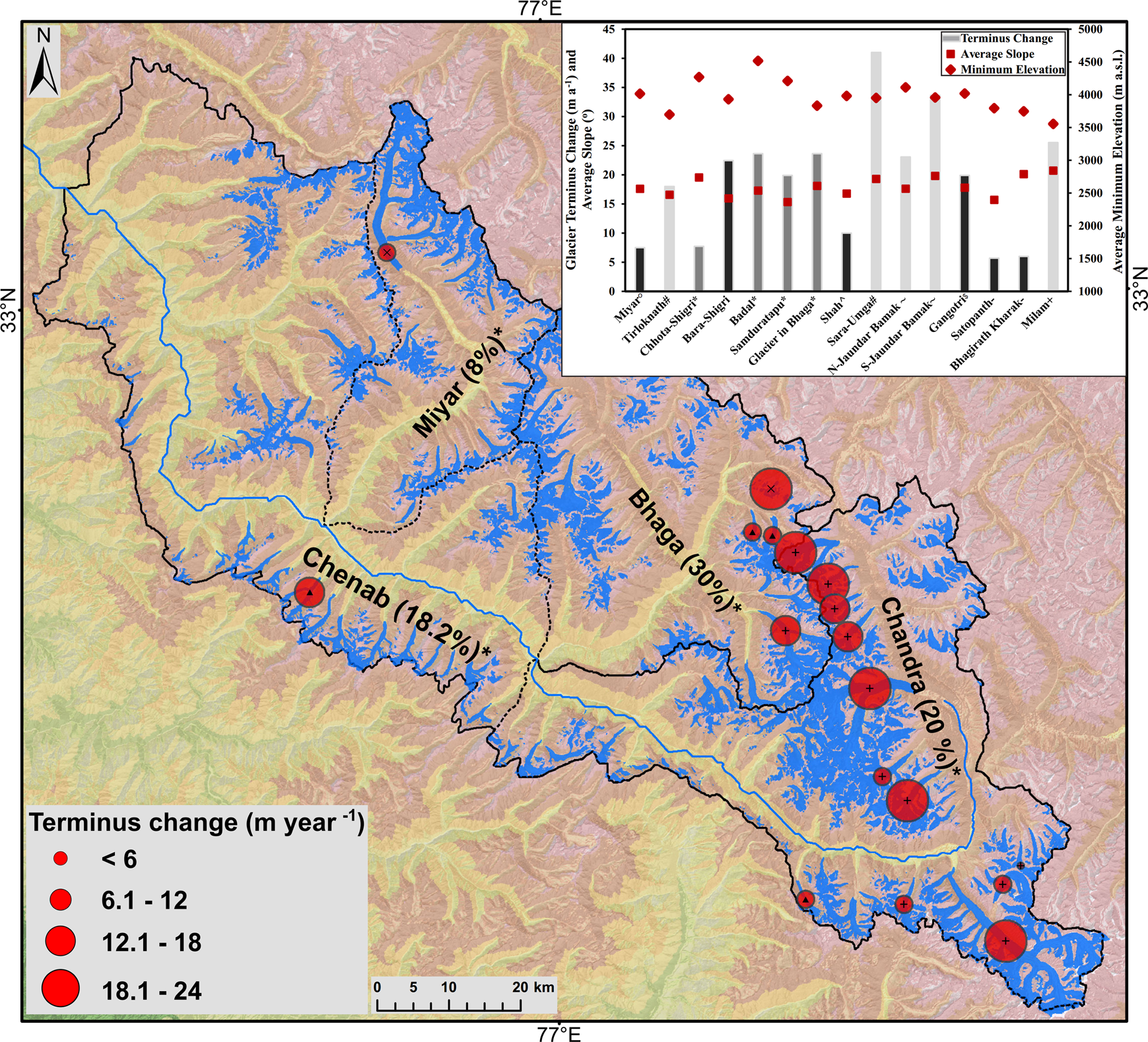
Reported frontal glacier area and terminus change for individual glaciers and overall for the sub-basins of Chenab where * represents the reference of Kulkarni et al. (2007). Symbols ×, + and ▴ represent the Corona, Landsat MSS image and SoI toposheets, respectively, used as historical datasets for glacier change detection. Inset figure shows the comparison of recession rate for the reported glacier terminus change for larger glacier during the past five/four decades and its correlation with minimum elevation and average slope in the Himachal and Central Himalaya. Most of the glacier shows variation in recession rates. Symbols ^O, #,*, ^, ∼, ^$, -, + show reference as Deswal et al. (in submission); Kulkarni and Karkatya (2014); Pandey and Venkataraman (2013); Chand and Sharma (2016); Mehta et al. (2012); Bhambri et al. (2012); Nainwal et al. (2016); Raj (2011), respectively.

The present study shows that repeat photographs provide immense opportunity to develop our understanding of contemporary impacts of climate change on the world’s highest mountain landscapes, especially when combined with other analytical tools such as remote sensing, GIS and especially field-based observations (Byers, 2008). In recent years, repeat photographs have been used for many glacier studies across the Himalayan region (Byers, 2008; Raina and Srivastava, 2008; Schmidt and Nüsser, 2009). For instance, Raina (2009) reported changes for a number of glaciers across the Indian Himalayan region based on repeated photographs. The study reported that the Sonapani Glacier in Chandra valley has retreated by about 500 m during the last 100 years; by comparison, the Kangriz Glacier in J&K Himalayas does not show any retreat. Similarly, the Siachen Glacier (1958–2008) in the Karakoram and the Machoi Glacier (1957–2007) in the J&K show an insignificant retreat in the last 50 years (Raina, 2009). Moreover, recent studies by Shukla et al. (2017) and Rashid et al. (2017) on the Kolahoi Glacier in the J&K Himalaya reported varying significant retreat of 3.4 km and 2.9 km, respectively, during 1857 to 2014. In addition, this technique was used for the Raikot and Chungphare glaciers in the Nanga Parbat massif (Nüsser and Schmidt, 2017; Schmidt and Nüsser, 2009), and to investigate glacial fluctuations in the Sagarmatha National Park (Mt Everest), Nepal (Byers, 2008). Moreover, a number of glaciers in the Himalaya have long historical records or archives in terms of repeated photographs and thus provide potential to produce detailed reconstructions of post-LIA glacier fluctuations (Raina, 2009; Raina and Srivastava, 2008). However, the main challenges with using repeat photographs is identifying photo locations, the accuracy of viewpoints, the congruence of the historical photographs, problems of visibility caused by shadows and clouds, the absence of camera specifications and capturing geometry, picture quality or resolution, and measurement of areas covered by snow or debris (Nüsser, 2000, 2001). However, the availability of advanced photography processing techniques/tools (e.g. plugins in AP CS-6), the well-identified signature of terrain elements and geomorphological features on the photo pairs, and their analytical interpretation with extensive validation in the field, has enhanced the accuracy of the approach. In addition, the recent availability of declassified high-resolution images from the Corona satellite provides an insight into glacier changes since the 1960s. Also, with the medium spatial resolution of Landsat TM/ETM+/OLI images with high spectral bands/contrast, the terminus and ice cliffs at glacier fronts can be detected, although with some limitations, especially when trying to differentiate sections of debris covered dead ice from the main trunk. This difficulty can often be overcome by field observations.

5.2. Climate and topographic control

Glacier dynamics are mainly driven by climatic parameters (e.g. temperature and precipitation), whereas topographic factors and surface characteristics can modulate this response (Benn et al., 2012; Bolch et al., 2008; Fujita, 2008; Furbish and Andrews, 1984; Haeberli, 1990). Previously, studies reported the advance of the Bara Shigri Glacier into the Shigri outwash plain during the ∼1830s (Egerton, 1864; Harcourt, 1871; Walker and Pascoe, 1907; Wilson, 1875), and the present study also indicates the impulsive advance of the Bara Shigri Glacier in the third or fourth half of early 19th century and ascribes this to the pooled results of climatic and non-climatic factors (e.g. glacier morphology, its steep frontal tributaries and valley topographical characteristics). For example, the study suggests cold climatic conditions during the late 18th century to early 19th century in different parts of the Himalaya (Grove, 2004; Xu and Yi, 2014). Yadav et al. (2004) reported cooling during the 1820s to 1850s in the western Himalaya, which coincides with cooling in central Asia and the Karakoram (Matthews and Briffa, 2005). Based on the analysis of annual snow accumulation record from the Guliya ice core (located ∼600 km north of the Bara Shigri Glacier; Figure 1a), Yao et al. (1996) suggested that, at the beginning of 19th century, an overall cooling phase started and the year 1820 was the coolest period since the 17th century. According to their study, the entire 19th century experienced low-precipitation, except in ∼1830, when precipitation was marginally increased. Xu and Yi (2014) reported glaciers throughout the TP, including glaciers from north-western Himalaya synchronously advancing during the late 18th to early 19th centuries, and suggested that the role of precipitation could have been a subsidiary, compared to the temperature, in driving glacier advance during the LIA. Borgaonkar et al. (2009) also observed a higher frequency of suppressed growth periods in tree rings in response to cooling and related this to positive glacial mass balance in the Himalayan region during the late 18th to early 19th centuries. Based on the regional climatic data proximal to the Bara Shigri Glacier, it is suggested that during the early 19th century the positive glacier mass balance was caused by cooler temperatures. This was exacerbated by a cumulative contribution from steep tributary glaciers which fed the main trunk glaciers, resulting in their advance from the confined glacial valleys into the open wide Shigri outwash plain (Figure 10). The steep tributary glaciers are well known to contribute a positive glacier mass balance and result in margin stability and/or further glacial advance (Barr and Lovell, 2014; Benn and Evans, 2010). Our study suggests that, during the second half of the early 19th century, positive mass balance and confined glacier valley morphology with steep frontal tributaries caused the glacier to advance rapidly in the open Shigri outwash plain and spread laterally to cross the Chandra river, forming piedmont lobes (Figure 10). These lobes and the lateral expansion of the glacier eventually dammed the Chandra river and formed the ice-dammed lake upstream for a considerable time, which later breached and caused devastating flooding downstream (e.g. Egerton, 1864; Harcourt, 1871; Walker and Pascoe, 1907). The notable decline in glacier surface area during the latter part of the mid-19th century (1863–1906) is represented by well-developed flutes, which otherwise would not have evolved in areas such as the Himalaya (Figure 2; Owen et al., 1996). In addition, relative stability at the margins eventually led the glacier to retreat within a confined/sheltered valley, and this is demonstrated by the presence of multiple latero-frontal or recessional moraines (Figures 2 and 10). Moreover, a unique assemblage of permafrost features (e.g. rock glaciers) in the basin indicates reduced moisture supply and overall changing climatic conditions during the late Holocene and LIA in this region (Owen and England, 1998); however, this needs further detailed investigation.

Figure 10.

Illustration shows the reported early 19th century advance of the Bara Shigri Glacier due to pooled results of lower temperatures during the early 19th century; glacier topographical characteristics and contribution from the frontal steep avalanching tributaries. (a) shows the Bara Shigri Glacier advance in the open piedmont Shigri outwash plain and extended across the Chandra river blocking it and forming ice-dammed lakes upstream of the right side of the glacier; (b) the slope map of the Bara Shigri Glacier basin as the frontal tributaries and glacial valley wall have a very steep slope, which further reflects from the inset picture of the profiles of confined topography in the frontal part of the glacier.

Our inference that increased temperature and reduced precipitation are responsible for the late 19th and 20th century glacier recession in Chandra valley finds support in the trends analysed from CRU data since 1900 (Figure 7a, c). Similar observations were made by Pant et al. (2003) and Bhutiyani et al. (2007, 2009), particularly after 1940, who note a marked increase in winter maximum and mean temperature (Pant et al., 2003; Borgaonkar et al., 2009) and decreasing rainfall over the western Himalaya, which was more significant after 1965 (Basistha et al., 2009). The western Himalayan tree ring data indicate that during 1945 to 1974 the warmest temperatures prevailed in the western Himalaya (Singh et al., 2005; Yadav and Singh, 2002). The climatic pattern inferred from the western Himalaya compares reasonably well with the regional data of climate variability post-LIA. For example, in the high-altitude areas of the TP, a warming trend was observed, particularly with winter temperature rising at 0.35°C per decade (Liu and Chen, 2000). The ice core isotope (δ⁸O) record of the Guliya and Dasuopu ice cores suggest appreciable warming during the 20th century (Thompson, 2000). Further, the Northern Hemispheric temperatures derived from high-resolution proxies such as tree ring and ice cores also indicate unprecedented warming in the 20th century (Mann et al., 1999). In view of this, it can be suggested that the post-LIA climate followed the global warming pattern, and frontal area changes of the Bara Shigri Glacier over the past five decades can be attributed to an increase in temperature and decrease in precipitation (inferences based on trends analysed from NCEP/NCAR data since ∼1950) (Figure 7e, f). In addition, recent decadal changes of the Bara Shigri Glacier can be attributed to a marginal decrease in snowfall during the last four decades, as also observed at the Tandi meteorological station (Figure 7b, d). A few recent studies from the western Himalaya, e.g. Rana et al. (2008) and Shekhar et al. (2010), indicate an overall decrease in the snowfall between 1984 to 2007. According to Shekhar et al. (2010) the seasonal average temperature (T_avg) over the western Himalaya has increased by 2°C with an increase of 2.8°C in annual T_max between 1984/85 and 2007/08, while annual T_min increased by about 1°C. The recent climate warming and coupled reduction in the snowfall is implicated as the driver of the negative mass balance in the adjoining Chhota Shigri and Hamtah glaciers during the last decade (Azam et al., 2012; Siddiqui and Maruthi, 2007; Vincent et al., 2013). Speculatively, the climatically induced negative mass balance could be responsible for the terminus recession, frontal area change and increase of debris cover for the Bara Shigri Glacier during the past few decades. However, there is an absence of long-term field-based meteorological datasets, and heterogeneity in the trend of climatic parameters on local and regional scales needs to be better understood to improve understanding of climatic impacts on glacier dynamics. In addition, the influence of non-climatic factors, e.g. topographical parameters as well as glacier morphology, thickness and distribution of debris-covered area and presence and development of supraglacial ponds, makes it difficult to determine the effects of climate on glacier fluctuations and needs further extensive field-based studies in terms of mass balance measurements with the incorporation of field observed meteorological datasets.

VI Conclusions

This study demonstrates the efficacy of repeated photographs and a multi-data integrated approach (MDIA) to infer long-term changes in glacier fluctuations since the end of LIA (1863–2014). The present study allows us to draw the following inferences.

The early 19th century advance of the Bara Shigri Glacier can be ascribed to the positive mass balance due to early 19th century cooling. In addition, glacier morphology, the confined shape of the glacial valley, the glacier’s topographic characteristics and the contribution from the steep avalanching tributaries in the frontal part of the glacier cumulatively aided the advance of the Glacier into the Shigri outwash plain.

The glacier receded continuously after the mid 19th century (1863) with a total average retreat of 2898 ± 50 m (19.2 ± 1.2 m a^-1) and a total area loss of 4 ± 1 km² in last 151 years (1863–2014). The recession after the mid 19th century is ascribed to the overall rising temperature and decreasing precipitation/snowfall in the region.

The above observations are also supported by high to medium resolution multi-temporal satellite datasets over the last half century (1965–2014), during which period the glacier lost a total frontal area of 1.1 ± 0.02 km², with an average terminus retreat of 1100 ± 32 m (23 ± 1 m a^-1).

Our estimates of the magnitude of the Bara Shigri Glacier fluctuations are inconsistent with previous studies, except with the few observations made by the GSI. The discrepancies are attributed to the use of coarse resolution remote sensing data (e.g. Landsat MSS) and the SoI topographic map in previous studies, which show higher frontal area changes when compared to our high to medium resolution satellite image-based study.

The study demonstrates the applicability of the MDIA technique and illustrates the usefulness of repeated photographs, historical archives/documents and geomorphological mapping, supplemented by extensive field observations, to reconstruct long-term, particularly post-LIA, glacier fluctuations in different parts of the Himalayan region where these sources are available.

Footnotes

Acknowledgements

We would like to thank GSI, Lucknow, for its web portal and for providing us reports, repeated photographs and sketch maps of the Bara Shigri Glacier. We also thank USGS for providing Landsat TM/ETM+/OLI and Corona data free of cost. We also thank Professor Iysten Barr for his valuable suggestions and improving the language and readability of the text. PC and MCS are grateful to Jawaharlal Nehru University, New Delhi, for providing the research facilities. RB thankfully acknowledges support from the Centre for Glaciology, Wadia Institute of Himalayan Geology. PC is grateful to Mr Ian Gilbert, DigitalGlobe Inc., and the DigitalGlobe 8 Band Challenge Committee for providing WorldView-2 satellite data at no cost. PC is also obliged to GSI, the people of Chandra valley and the shepherds for their support during field work.

Declaration of Conflicting Interests

The authors declared no potential conflicts of interest with respect to the research, authorship, and/or publication of this article.

Funding

The authors received no financial support for the research, authorship, and/or publication of this article.

References

Agrawal

Sharma

Tayal

(2014) Assessment of regional climatic changes in the Eastern Himalayan region: a study using multi-satellite remote sensing data set. Environmental Monitoring and Assessment 186: 6521–6536. doi: 10.1007/s10661-014-3871-x

Ali

Biswas

Shukla

. (2013) Chronology and climatic implications of Late Quaternary glaciations in the Goriganga valley, central Himalaya, India. Quaternary Science Reviews 73: 59–76. doi: 10.1016/j.quascirev.2013.05.016

Arendt

Bliss A

Bolch

. (2014) Randolph Glacier Inventory [v4]: a dataset of global glacier outlines. Boulder, Colorado: Global Land Ice Measurements from Space.

Auden

(1937) Snout of the Gangotri Glacier, Tehri Garhwal. Records of the Geological Survey of India 72: 135–140.

Azam

Wagnon

Ramanathan

. (2012) From balance to imbalance: a shift in the dynamic behaviour of Chhota Shigri glacier, western Himalaya, India. Journal of Glaciology 58: 315–324. doi: 10.3189/2012JoG11J123

Azam

Wagnon

Vincent

. (2014) Reconstruction of the annual mass balance of Chhota Shigri Glacier, Western Himalaya, India, since 1969. Annals of Glaciology 55: 69–80. doi: 10.3189/2014AoG66A104

Bali

Nawaz Ali

Agarwal

. (2013) Chronology of late Quaternary glaciation in the Pindar valley, Alaknanda basin, Central Himalaya (India). Journal of Asian Earth Sciences 66: 224–233. doi: 10.1016/j.jseaes.2013.01.011

Bandyopadhyay

(1983) Recent advance and retreat of Bara Shigri Glacier of Eastern Lahaul. In: Proceedings of the First National Symposium on Seasonal Snow Cover, New Delhi, Vol. II, pp. 121–125.

Barnard

Owen

Finkel

(2004) Style and timing of glacial and paraglacial sedimentation in a monsoon-influenced high Himalayan environment, the upper Bhagirathi valley, Garhwal Himalaya. Sedimentary Geology 165: 199–221. doi: 10.1016/j.sedgeo.2003.11.009

10.

Barr

Lovell

(2014) A review of topographic controls on moraine distribution. Geomorphology 226: 44–64. doi: 10.1016/j.geomorph.2014.07.030

11.

Basistha

Arya

Goel

(2009) Analysis of historical changes in rainfall in the Indian Himalayas. International Journal of Climatology 29(4): 555–572.

12.

Benn

Bolch

Hands

. (2012) Response of debris-covered glaciers in the Mount Everest region to recent warming, and implications for outburst flood hazards. Earth-Science Reviews 114(1–2): 156–174.

13.

Benn

Evans

DJA

(2010) Glaciers and Glaciation, 2nd edn. Abingdom, UK: Hodder Arnold Publication.

14.

Bhambri

Bolch

(2009) Glacier mapping: a review with special reference to the Indian Himalayas. Progress in Physical Geography 33: 672–704. doi: 10.1177/0309133309348112

15.

Bhambri

Bolch

Chaujar

(2012) Frontal recession of Gangotri Glacier, Garhwal Himalayas, from 1965 to 2006, measured through high resolution remote sensing data. Current Science 102: 1462–1466.

16.

Bhambri

Bolch

Chaujar

. (2011) Glacier changes in the Garhwal Himalaya, India, from 1968 to 2006 based on remote sensing. Journal of Glaciology 57: 543–556. doi: 10.3189/002214311796905604

17.

Bhambri

Bolch

Kawishwar

. (2013) Heterogeneity in glacier response in the upper Shyok valley, northeast Karakoram. The Cryosphere 7: 1385–1398. doi: 10.5194/tc-7-1385-2013

18.

Bhutiyani

Kale

Pawar

(2007) Long-term trends in maximum, minimum and mean annual air temperatures across the Northwestern Himalaya during the twentieth century. Climate Change 85: 159–177. doi: 10.1007/s10584-006-9196 -1

19.

Bhutiyani

Kale

Pawar

(2009) Climate change and the precipitation variations in the northwestern Himalaya: 1866–2006. International Journal of Climatology 30: 535–548. doi: 10.1002/joc.1920

20.

Bisht

Ali

Shukla

. (2015) Chronology of late Quaternary glaciation and landform evolution in the upper Dhauliganga valley, (Trans Himalaya), Uttarakhand, India. Quaternary Science Reviews 129: 147–162. doi: 10.1016/j.quascirev.2015.10.017

21.

Bolch

Buchroithner

Pieczonka

. (2008) Planimetric and volumetric glacier changes in the Khumbu Himal, Nepal, since 1962 using Corona, Landsat TM and ASTER data. Journal of Glaciology 54(187): 592–600.

22.

Bolch

Kulkarni

Kääb

. (2012) The state and fate of Himalayan glaciers. Science 336(80): 310–314. doi: 10.1126/science.1215828

23.

Bolch

Menounos

Wheate

(2010a) Landsat-based inventory of glaciers in western Canada, 1985–2005. Remote Sensing of Environment 114: 127–137. doi: 10.1016/j.rse.2009.08.015

24.

Bolch

Yao

Kang

. (2010b) A glacier inventory for the western Nyainqentanglha range and the Nam Co basin, Tibet, and glacier changes 1976–2009. The Cryosphere 4: 419–433. doi: 10.5194/tc-4-419-2010

25.

Borgaonkar

Ram

Sikder

(2009) Assessment of tree ring analysis of high-elevation Cedrus deodara D. Don from Western Himalaya (India) in relation to climate and glacier fluctuations. Dendrochronologia 27: 59–69. doi: 10.1016/j.dendro.2008.09.002

26.

Bradley

Jonest

(1993) ‘Little Ice Age’ summer temperature variations: their nature and relevance to recent global warming trends. The Holocene 3: 367–376. doi: 10.1177/095968369300300409

27.

Byers

(2008) An assessment of contemporary glacier fluctuations in Nepal’s Khumbu Himal using repeat photography. Himalayan Journal of Science 4: 21–26. doi: 10.3126/hjs.v4i6.979

28.

Chand

Sharma

(2015a) Glacier changes in the Ravi basin, north-western Himalaya (India) during the last four decades (1971–2010/13). Global and Planetary Change 135: 133–147. doi: 10.1016/j.gloplacha.2015.10.013

29.

Chand

Sharma

(2015b) Frontal changes in the Manimahesh and Tal glaciers in the Ravi basin, Himachal Pradesh, northwestern Himalaya (India), between 1971 and 2013. International Journal of Remote Sensing 36: 4095–4113.

30.

Chand

Sharma

(2016) Monitoring frontal changes of Shah Glacier in the Ravi basin, Himachal Himalaya (India) from 1965 to 2013. National Academy of Science Letters 39: 109–114. doi: 10.1007/s40009-016-0420-x

31.

Chudley

Miles

Willis

(2017) Glacier characteristics and retreat between 1991 and 2014 in the Ladakh range, Jammu and Kashmir. Remote Sensing Letters 8: 518–527. doi: 10.1080/2150704X.2017.1295480

32.

Cotter G de

Brown

(1907) Notes on certain glaciers in Kumaon. Records of the Geological Survey of India 35: 148–157.

33.

Crowley

(2000) Causes of climate change over the past 1000 years. Science 289 (80): 270–277. doi: 10.1126/science.289.5477.270

34.

Deswal

Sharma

Saini

. (In Submission) Recession Pattern of Glaciers in Miyar Basin, Lahaul Himalaya, North-West India During Last Five Decades (1965–2015). Progress in Physical Geography: In Submission.

35.

Dortch

Owen

Caffee

(2013) Timing and climatic drivers for glaciation across semi-arid western Himalayan–Tibetan orogen. Quaternary Science Reviews 78: 188–208. doi: 10.1016/j.quascirev.2013.07.025

36.

Dutt

(1961) The Bara-Shigri Glacier, Kangra district, east Punjab, India. Journal of Glaciology 3(30): 1007–1015.

37.

Dutt

Ahmad

(1957) Report on the Bara Shigri glacier, Kangra, East Punjab and on the Geology of the Adjacent Area. Lucknow, Uttar Pradesh, India: GSI.

38.

Eddy

(1976) The maunder minimum. Science 192: 1189–202. doi: 10.1126/science.192.4245.1189

39.

Egerton

(1864) Journal of a Tour Through Spiti to the Frontier of Chinese Thibet. London: Cundall Downs.

40.

Finsterwalder

(1935) On the map of the Zemu Glacier. Himalayan Journal 7: 125–138.

41.

Finsterwalder

Pillewizer

(1937) Photogrammetric studies of glaciers of High Asia. Himalayan Journal 11: 107–113.

42.

Frey

Paul

Strozzi

(2012) Compilation of a glacier inventory for the western Himalayas from satellite data: methods, challenges, and results. Remote Sensing Environment 124: 832–843. doi: 10.1016/j.rse.2012.06.020

43.

Fujita

(2008) Effect of precipitation seasonality on climatic sensitivity of glacier mass balance. Earth and Planetary Science Letters 276(1–2): 14–19.

44.

Furbish

Andrews

(1984) The use of hypsometry to indicate long-term stability and response of valley glaciers to changes in mass transfer. Journal of Glaciology 30(105): 199–211.

45.

Garg

Shukla

Tiwari

. (2017) Assessing the status of glaciers in part of the Chandra basin, Himachal Himalaya: a multiparametric approach. Geomorphology 284: 99–114. doi: 10.1016/j.geomorph.2016.10.022

46.

Godwin-Austen

(1864) On the glaciers of the Mustagh range. Journal of the Royal Geographical Society 34: 19–56.

47.

Granshaw

Fountain

(2006) Glacier change (1958–1998) in the North Cascades National Park Complex, Washington, USA. Journal of Glaciology 52: 251–256.

48.

Grove

(1988) The Little Ice Age. London: Methuen and Co. Ltd.

49.

Grove

(2004) ‘Little Ice Ages’: ancient and modern, vols I and II . London: Routledge.

50.

GSI (1997) Annual General Report. General Survey of India.

51.

GSI (2000) Annual General Report. General Survey of India.

52.

Haeberli

(1990) Glacier and permafrost signals of 20th-century warming. Annals of Glaciology 4(1): 99–101.

53.

Hall

Bayr

Schöner

. (2003) Consideration of the errors inherent in mapping historical glacier positions in Austria from the ground and space (1893–2001). Remote Sensing Environment 86: 566–577.

54.

Hannesdóttir

Björnsson

Pálsson

. (2014) Variations of southeast Vatnajökull ice cap (Iceland) 1650–1900 and reconstruction of the glacier surface geometry at the Little Ice Age maximum. Geografiska Annaler Series A, Physical Geography November: pp. 28. doi: 10.1111/geoa.12064

55.

Harcourt

AFP

(1871) On the Himalayan valleys: Kooloo, Lahoul, and Spiti. Proceedings of the Royal Geogaphicalr Society of London 15: 336–343.

56.

Hastenrath

(2008) Recession of Equatorial Glaciers: A Photo Documentation. Madison, WI: Sundog Publishing, p. 142.

57.

Hewitt

(2011) Glacier change, concentration and elevation effects in the Karakoram Himalaya, Upper Indus Basin. Mountain Research and Development 31: 188–200. doi: 10.1659/MRD-JOURNAL-D-11-00020.1

58.

Hodgson

(1822) Journal of a survey to the heads of the rivers Ganges and Jumna. Asiatic Resolutions 14: 60–152.

59.

Hubbard

Glasser

(2005) Field Techniques in Glaciology and Glacial Geomorphology. UK: Wiley-Blackwell.

60.

IPCC (2007) Summary for policymakers: the physical science basis. Contribution of Working Group I to the Fourth Assessment Report of the Intergovernmental Panel on Climate Change.

61.

IPCC Working Group 1, Stocker

Qin

. (2013) Climate change 2013: the physical science basis. Contribution of Working Group I to the Fifth Assessment Report of the Intergovernmental Panel on Climate Change.

62.

Kamp

Byrne

Bolch

(2011) Glacier fluctuations between 1975 and 2008 in the Greater Himalaya Range of Zanskar, southern Ladakh. Journal of Mountain Science 8: 374–389. doi: 10.1007/s11629-011-2007-9

63.

Kamp

McManigal

Dashtseren

. (2013) Documenting glacial changes between 1910, 1970, 1992 and 2010 in the Turgen mountains, Mongolian Altai, using repeat photographs, topographic maps and satellite imagery. Geographical Journal 179: 248–263. doi: 10.1111/j.1475-4959.2012.00486.x

64.

Krenek

Bhawan

(1945) Recent and past glaciation of Lahaul. Indian Geographical Journal 20(3): 93–102.

65.

Kulkarni

Karyakarte

(2014) Observed changes in Himalayan glaciers. Current Science 106: 237–244.

66.

Kulkarni

Bahuguna

Rathore

. (2007) Glacial retreat in Himalaya using Indian remote sensing satellite data. Current Science 92: 69–74.

67.

Kumar

Singh

Singh Randhawa

. (2014) Temperature trend analysis in the glacier region of Naradu valley, Himachal Himalaya, India. Comptes Rendus Geoscience 346: 213–222. doi: 10.1016/j.crte.2014.09.001

68.

Liu

Chen

(2000) Climatic warming in the Tibetan Plateau during recent decades. International Journal of Climatology 20(14): 1729–1742.

69.

Loibl

Lehmkuhl

Grießinger

(2014) Reconstructing glacier retreat since the Little Ice Age in SE Tibet by glacier mapping and equilibrium line altitude calculation. Geomorphology 214: 22–39. doi: 10.1016/j.geomorph.2014.03.018

70.

Longstaff

(1910) Glacier exploration in the eastern Karakoram. Geographical Journal 35: 622–658.

71.

Lowell

(2000) As climate changes, so do glaciers. Proceedings of the National Acadamy of Sciences of the United States of America 97: 1351–1354.

72.

Mann

(2002) Little Ice Age. In: MacCracken

DMC

Perry

(eds) Encyclopedia of Global Environmental Change. UK: John Wiley & Sons, 504–509.

73.

Mann

Bradley

Hughes

(1999) Northern hemisphere temperatures during the past millennium: inferences, uncertainties, and limitations. Geophysical Research Letters 26: 759–762. doi: 10.1029/1999GL900070

74.

Mann

Cane

Zebiak

. (2005) Volcanic and solar forcing of the tropical Pacific over the past 1000 years. Journal of Climate 18: 447–456.

75.

Mason

(1914) The Indo-Russian triangulation connection. Geographical Journal 43: 664–672.

76.

Mason

(1927a) The stereographic survey of the Shaksgam. Geographical Journal 70: 342–352.

77.

Mason

(1927b) The Shaksgam valley and Aghil range. Geographical Journal 69: 289–323.

78.

Mason

(1928) Note on Sir Francis Younghusband’s Urdok Glacier. Mason K (1914) The Indo-Russian triangulation connection. Geographical Journal 71: 275–277.

79.

Matthes

(1939) Report of the committee on glaciers, April 1939. Transactions of the American Geophysical Union Journal 20: 518–523.

80.

Matthews

Briffa

(2005) The ‘Little Ice Age’: re-evaluation of an evolving concept. Geografiska Annaler Series A, Physical Geography 87: 17–36. doi: 10.1111/j.0435-3676.2005.00242.x

81.

Mayewski

Jeschke

(1979) Himalayan and Trans-Himalayan glacier fluctuations since AD 1812. Arctic, Antarctic and Alpine Research 11: 267–287.

82.

Mir

Majeed

(2016) Frontal recession of Parkachik Glacier between 1971–2015, Zanskar Himalaya using remote sensing and field data. Geocarto International 31: 1–15. doi: 10.1080/10106049.2016.1232439

83.

Mumm

(1909) Five Months in the Himalaya: A Record of Mountain Travel in Garhwal and Kashmir. UK: Longmans Green.

84.

Nainwal

Banerjee

Shankar

. (2016) Shrinkage of Satopanth and Bhagirath Kharak glaciers, India, from 1936 to 2013. Annals of Glaciology 57: 131–139.

85.

Nüsser

(2000) Change and persistence: contemporary landscape transformation in the Nanga Parbat region, Northern Pakistan. Mountain Research and Development 20: 348–355. doi: 10.1659/0276-4741(2000)020[0348: CAPCLT]2.0.CO;2

86.

Nüsser

(2001) Understanding cultural landscape transformation: a re-photographic survey in Chitral, eastern Hindukush, Pakistan. Landscape and Urban Planning 57: 241–255. doi: 10.1016/S0169-2046(01)00207-9

87.

Nüsser

Schmidt

(2017) Nanga Parbat revisited: evolution and dynamics of sociohydrological interactions in the Northwestern Himalaya. Annals of the Association of American Geographers 107: 403–415. doi: 10.1080/24694452.2016.1235495

88.

Oerlemans

(2005) Extracting a climate signal from 169 glacier records. Science 308: 675–677. doi: 10.1126/science.1107046

89.

Owen

Dortch

(2014) Nature and timing of Quaternary glaciation in the Himalayan–Tibetan orogen. Quaterary Science Reviews 88: 14–54. doi: 10.1016/j.quascirev.2013.11.016

90.

Owen

England

(1998) Observations on rock glaciers in the Himalayas and Karakoram Mountains of northern Pakistan and India. Geomorphology 26: 199–213. doi: 10.1016/S0169-555X(98)00059-2

91.

Owen

Derbyshire

Richardson

. (1996) The Quaternary glacial history of the Lahul Himalaya, northern India. Journal of Quaternary Science 11: 25–42. doi: 10.1002/(SICI)1099-1417(199601/02)11:1<25:: AID-JQS209>3.0.CO;2-K

92.

Owen

Gualtieri

LYN

Finkel

. (2001) Cosmogenic radionuclide dating of glacial landforms in the Lahul Himalaya, northern India: defining the timing of Late Quaternary glaciation. Journal of Quaternary Science 16: 555–563. doi: 10.1002/jqs.621

93.

Pandey

Ghosh

Nathawat

(2011) Evaluating patterns of temporal glacier changes in Greater Himalayan range, Jammu & Kashmir, India. Geocarto International 26: 321–338. doi: 10.1080/10106049.2011.554611

94.

Pandey

Nathawat

Ghosh

(2012) Morphometric control on glacier area changes in the Great Himalayan range, Jammu and Kashmir, India. Current Science 102: 1188–1193.

95.

Pandey

Venkataraman

(2013) Changes in the glaciers of Chandra–Bhaga basin, Himachal Himalaya, India, between 1980 and 2010 measured using remote sensing. International Journal of Remote Sensing 34: 5584–5597. doi: 10.1080/01431161.2013.793464

96.

Pant

Borgaonkar

Rupa Kumar

(2003) Climate variability over the Western Himalaya since the Little Ice Age: dendroclimatic implications. Jalvigyan Sameeksha. Hydrology Review 18: 111–121.

97.

Paul

Svoboda

(2009) A new glacier inventory on southern Baffin Island, Canada, from ASTER data: II. Data analysis, glacier change and applications. Annals of Glaciology 50: 22–31.

98.

Paul

Barrand

Baumann

. (2013) On the accuracy of glacier outlines derived from remote sensing data. Annals of Glaciology 54: 171–182. doi: 10.3189/2013AoG63A296

99.

Paul

Barry

Cogley

. (2010) Guidelines for the compilation of glacier inventory data from digital sources. Available at: http://globglacier.ch/docs/guidelines_inventory.pdf (accessed 10 August 2017).

100.

Paul

Kääb

Maisch

. (2002) The new remote sensing-derived Swiss glacier inventory: I. Methods. Annals of Glaciology 34: 355–361. doi: 10.3189/172756402781817941

101.

Racoviteanu

Williams

Barry

(2008) Optical remote sensing of glacier characteristics: a review with focus on the Himalaya. Sensors 8: 3355–3383. doi: 10.3390/s8053355

102.

Raina

Srivastava

(2008) Glacier Atlas of India. Bangalore: GSI.

103.

Raina

(2009) Himalayan glaciers: a state-of-art review of glacial studies, glacial retreat and climate change. Delhi: GSI.

104.

Raj

KBG

(2011) Recession and reconstruction of Milam Glacier, Kumaon Himalaya, observed with satellite imagery. Current Science 100: 1420–1425.

105.

Rana

Bhagat

Kalia

. (2008) Impact of climate change on shift of apple belt in Himachal Pradesh. In: ISPRS Archives XXXVIII-8/W3 Workshop Proceedings: Impact of Climate Change on Agriculture, pp. 131–137. Available at: http://www.isprs.org/proceedings/XXXVIII/8-W3/b2/10-B10-179_ISRO%20F.pdf

106.

Rashid

Romshoo

Abdullah

(2017) The recent deglaciation of Kolahoi valley in Kashmir Himalaya, India, in response to the changing climate. Journal of Asian Earth Sciences 138: 38–50. doi: 10.1016/j.jseaes.2017.02.002

107.

Raup

Kääb

Kargel

. (2007) Remote sensing and GIS technology in the Global Land Ice Measurements from Space (GLIMS) Project. Computers & Geosciences 33: 104–125. doi: 10.1016/j.cageo.2006.05.015

108.

Rawat

Vishvakarma

SCR

Todaria

(2009) Fuel wood consumption pattern of tribal communities in cold desert of the Lahaul valley, North-Western Himalaya, India. Biomass and Bioenergy 33: 1547–1557. doi: 10.1016/j.biombioe.2009.07.019

109.

Sangewar

(1995) Glacier front fluctuation studies in parts of Himachal Pradesh and Uttar Pradesh. Records Geological Survey of India 129: 218–219.

110.

Sati

Ali

Rana

. (2014) Timing and extent of Holocene glaciations in the monsoon dominated Dunagiri valley (Bangni Glacier), Central Himalaya, India. Journal of Asian Earth Sciences 91: 125–136. doi: 10.1016/j.jseaes.2014.05.008

111.

Schauwecker

Rohrer

Huggel

. (2015) Remotely sensed debris thickness mapping of Bara Shigri Glacier, Indian Himalaya. Journal of Glaciology 61: 675–688.

112.

Schmidt

Nüsser

(2009) Fluctuations of Raikot Glacier during the past 70 years: a case study from the Nanga Parbat massif, northern Pakistan. Journal of Glaciology 55: 949–959. doi: 10.3189/002214309790794878

113.

Schmidt

Nüsser

(2012) Changes of high altitude glaciers from 1969 to 2010 in the Trans-Himalayan Kang Yatze massif, Ladakh, Northwest India. Arctic, Antarctic and Alpine Research 44: 107–121. doi: http://dx.doi.org/10.1657/1938-4246-44.1.107

114.

Schmidt

Nüsser

(2017) Changes of high altitude glaciers in the Trans-Himalaya of Ladakh over the past five decades (1969–2016). Geosciences 7: 27. doi: 10.3390/geosciences7020027

115.

Sharma

Owen

(1996) Quaternary glacial history of NW Garhwal, Central Himalayas. Quaternary Science Reviews 15: 335–365. doi: 10.1016/0277-3791(95)00061-5

116.

Shekhar

Chand

Kumar

. (2010) Climate change studies in the western Himalaya. Annals of Glaciology 51: 105–112. doi: 10.3189/172756410791386508

117.

Shukla

Qadir

(2016) Differential response of glaciers with varying debris cover extent: evidence from changing glacier parameters. International Journal of Remote Sensing 37: 2453–2479. doi: 10.1080/01431161.2016.1176272

118.

Shukla

Ali

Hasan

. (2017) Dimensional changes in the Kolahoi Glacier from 1857 to 2014. Environmental Monitoring and Assessment 189: 5. doi: 10.1007/s10661-016-5703-7

119.

Siddiqui

Maruthi

(2007) Detailed glaciological studies on Hamtah Glacier, Lahaul and Spiti District, HP. Geological Survey of India 140: 92–93.

120.

Singh

Park

W-K

Yadav

(2005) Tree ring-based hydrological records for western Himalaya, India, since AD 1560. Climate Dynamics 26: 295–303. doi: 10.1007/s00382-005-0089 -1

121.

Srikantia

Padhi

(1964) Report on the Bara-Shigri Glacier, Lahaul-Spiti district, Punjab. Report of Geological Survey of India, Lucknow, Uttar Pradesh, India, pp. 23. Available at: http://www.portal.gsi.gov.in/gsiDoc/fspReports/NRO/1960-1965/NRO_20088_1962_1963_REPORT_1.pdf

122.

Strachey

(1847) A description of the glaciers of the Pindur and Kuphinee rivers in the Kumaon Himalaya. Journal of the Asiatic Society of Bengal 16: 794–812.

123.

Swaroop

Shukla

(1999) Glacier Front Fluctuation Studies in Parts of Himachal Pradesh and Uttar Pradesh. Report of Geological Survey of India, Lucknow, Uttar Pradesh, India, pp. 27. Available at: http://www.portal.gsi.gov.in/portal/page?_pageid=108,721670&_dad=portal&_schema=PORTAL

124.

Thompson

(2000) Ice core evidence for climate change in the tropics: implications for our future. Quaternary Science Reviews 19: 19–35. doi: 10.1016/S0277-3791(99)00052-9

125.

Tobler

(1987) Measuring Spatial Resolution, Proceedings, Land Resources Information Systems Conference, Beijing, 1987, pp. 12–16. Available at: http://www.geog.ucsb.edu/∼tobler/publications/published.html

126.

Vincent

Ramanathan

Wagnon

. (2013) Balanced conditions or slight mass gain of glaciers in the Lahaul and Spiti region (northern India, Himalaya) during the nineties preceded recent mass loss. The Cryosphere 7: 569–582. doi: 10.5194/tc-7-569-2013

127.

Visser

(1926) Explorations in the Karakoram. Geographical Journal 68: 457–468.

128.

Visser

(1934) The Karakoram and Turkestan expedition of 1929–1930. Geographical Journal 84: 281–295.

129.

Walker

Pascoe

(1907) Notes on certain glaciers in Lahaul. Records of the Geological Survey of India 35: 139–147.

130.

Webb

(2007) The Desert Laboratory Repeat Photography Collection: an invaluable archive documenting landscape change. Fact Sheet 2007-3046. Reston.

131.

WGMS (2008) Fluctuation of Glaciers 2000–2005, vol. IX. Zürich: WGMS.

132.

Wilson

(1875) The Abode of Snow . London: William Blackwood and Sons.

133.

Workman

(1906) First exploration of the Hoh Lumba and Sosbon glaciers: two pioneer ascents in the Himalayas. Geographical Journal 27 :129–141.

134.

(2014) Little Ice Age on the Tibetan Plateau and its bordering mountains: Evidence from moraine chronologies. Global and Planetary Change 116: 41–53. doi: 10.1016/j.gloplacha.2014.02.003

135.

Yadav

Park

W-K

Singh

. (2004) Do the western Himalayas defy global warming? Geophysical Research Letters 31(17): 1–5.

136.

Yadav

Singh

(2002) Tree-Ring-Based Spring Temperature Patterns over the Past Four Centuries in Western Himalaya. Quaternary Research 57(3): 299–305.

137.

Yao

Keqin

Lide

. (1996) Climatic variations since the Little Ice Age recorded in the Guliya Ice Core. Science China Series D 39: 587–596.

138.

Zängl and Hamberger (2004) Gletscher im Treibhaus : Eine fotografische Zeitreise in die alpine Eiswelt. Tecklenborg Verlag, Steinfurth.