Effects of environmental and turbine parameters on energy gains from wind farm system: Artificial neural network simulations

Abstract

Artificial neural network modelling has been employed to investigate the effects of various environmental and machine factors on the energy gain from wind farm systems. Numerical comparison of artificial neural network and nonlinear regression from XLSTAT showed that ANN possessed better numerical accuracy in predicting multivariate data. Several artificial neural network models are developed and tested with several structures to obtain the best prediction performance in energy gain from different wind farms in Jordan. The best performing artificial neural network model was used to predict the energy gain from wind farm based on changes in annual wind speed, turbine rotor diameter and turbine power. As a result of 20% increase in turbine power, 14.4%–31% energy gains were recorded across different wind farms. The proposed artificial neural network model was also a good predictor for energy cost resulting from specific wind farm design.

Keywords

Artificial neural network wind farm wind turbine energy gains rotor diameter

Introduction

The world continues to be heavily dependent on fossil fuel as the main source of energy. However, two very strong notions have become paramount for planning future energy production: fossil fuel’s environmental ill effects, and the impending depletion of fossil fuel reserves. Both of these factors are driving global interest in the identification of clean, sustainable sources of energy. Developments over the past few decades have identified wind as an important alternative – under appropriate climatic and geographical settings. As a result, wind energy systems have been deployed in numerous countries across the globe, both developed and developing (Ammariet al., 2014).One of these countries is Jordan, with vast arid areas and paltry oil resources (Alghoul et al., 2007; Anani et al., 1998; Habali et al., 1987).

Technical assessments of wind farm systems’ performance in many areas of Jordan have already been reported in the literature. For example, Ammariet al. (2014) evaluated the electrical energy derivable from wind at different existing wind farms in Jordan. Several factors were considered in the analyses, which included environmental factors (i.e. mean monthly and annual wind speeds at different geographical locations) as well as systemic factors (i.e. characteristics of the different wind turbines employed at the different locations). Their findings indicate that sites with high mean wind speed have better promise of energy output. Other researchers have also corroborated the strong correlation between wind speed and power output (Ackeret al., 2007). Bataineh and Dalalah (2013) performed a technical assessment of wind power potential at seven different locations in Jordan. They used Rayleigh distribution to model the monthly average wind data at the different locations. Using wind turbines of different capacities, the work estimated energy output potential for the selected sites. Energy cost analyses were also performed. The results showed cost-effectiveness of energy generation from the selected sites, with unit cost less than US$0.04/kWh. Along the same lines, a work was carried out in the context of an energy diversification drive for Jordan with the inclusion of the eastern part of the country (Ammariet al., 2014). The work evaluated energy gains (EV) and capacity factor as consequences of the environmental and systemic factors mentioned above. The investigations were carried out at five locations – different from those considered by Bataineh and Dalalah (2013). Also, Ammari et al. (2014) utilized turbine capacities ranging from 100 to 3000 kW, while the investigations of Bataineh and Dalalah (2013) used turbines with capacities between 1650 and 3000 kW.

All of the works mentioned above are based on costly time-consuming field investigations. These expenses limit the amount of experimental exploration possible on the factors influencing the operation and efficiency of the wind farm systems. In addition, elaborate experimental investigations might be laden with inconsistencies as a result of unavoidable errors. An efficient modelling system is needed to mitigate the cost and delays involved in such field investigations. The modelling system will allow the exploration of other salient features of the experimental findings as well as the influences of numerous variables that affect EV from wind turbine.

Such a modelling system needs to be based on computational descriptions of the data as well as quantitative description of patterns of EV, together with influential factors in the wind farm system. Such a platform should have the ability to interpret and assimilate multifarious data of diverse origins together with the understanding of behavioural trends in output quantities, based on the different input variables. Thus, the model needs to have the ability to predict such trends in regions beyond the experimental ranges. Many computational techniques useful under these circumstances are available. These techniques, however, often require complex procedures to set up and run (Abidoye and Das, 2015; Hanspal et al., 2013; Spalding, 1981).

Thus, there is a need for inexpensive, easy-to-use tools that can easily assist investigators in determining intricate relationships among several interrelated variables. It has been shown that artificial neural networks (ANNs) are able to demonstrate the required mathematical properties needed for modelling such systems (Ammari et al., 2014; Anani et al., 1998; Bani-Hani and Abidoye, 2016; Bataineh and Dalalah, 2013; Das et al., 2014). ANN is a well-known modelling tool. It possesses the ability to learn and generalize functions from rounds of training as well as extract essential information from data (Abidoye and Das, 2015; Khashei and Bijari, 2014; Zhanget al., 1998). ANN modelling utilizes building blocks or elements called ‘neurons’. The neurons are grouped into input, hidden and output layers with respective biases, weights and transfer functions (Abidoye and Das, 2015; Yurdakul and Akdas, 2013; Mueller and Hemond, 2013). The network manipulates the values of the biases and weights in a sequence of training processes and uses the transfer functions to establish the relationships between the inputs and the outputs. ANNs are currently being applied in many fields for a variety of complex modelling tasks (Widrow, 1962). ANNs are data-driven, self-adaptive methods in that they learn from rounds of training and capture subtle functional relationships among the data even if the underlying relationships among the parameters are unknown or hard to describe (Zhang et al., 1998). Thus, if enough data are available, the solution can be obtained by treating the problem as one of the multivariate, nonlinear, nonparametric, statistical methods (White, 1989).The adaptive learning algorithms of ANN give it the capacity to handle diverse types of data and integrate them into categorized outputs (Amato et al., 2013). ANN has been applied to model renewable energy systems, economics, psychology, subsurface two-phase flow and many more (Abidoye and Bello, 2017; Abidoye and Das, 2015; Kalogirou, 1999). Authors like Petković et al. (2015) have suggested soft computing for wind farm analysis. Soft and simplified computational techniques will overcome the cost and complexity associated with flow-physics-based computational fluid dynamic (CFD) simulators that are employed in works like that of Das et al. (2014) and Abidoye and Wairagu (2013). Muyeen et al. (2014) used the superconducting magnetic energy storage (SMES) system to enhance the transient stability of wind farms connected to multi-machine power system during network disturbances. The SMES was controlled by adaptive ANN.

This work explores the capabilities of ANN to model the complex relationships that exist between environmental and system variables affecting the EV from wind farms. It will be shown that the modelling parameters involved in the quantitative descriptions of EV from wind turbine are interrelated in a complex manner. Since ANN can approximate the relevant functions to the desired accuracy (Hanspal et al., 2013; Abidoye and Mahdi (2014); Zhang et al., 1998), it is believed that logical arrangement and tabulation of the variables will enhance the training, validation, testing as well as prediction of the existing interrelationships. This approach stems from the realization that a well-trained and validated ANN structure can give reliable prediction (Hanspal et al., 2013).

To ensure fair numerical comparison and performance evaluation, this work also investigates the numerical performance of nonlinear regression, using the software XLSTAT 2017 from Addinsoft. The work will also establish the comparative advantage of ANN over XLSTAT.

Methodology

The methodology employed in this work is to use statistical modelling tools for quantitative description of the effects of various environmental and system parameters on the amount of EV from wind turbines of various capacities at different locations in Jordan. The modelling tools utilized are ANN and nonlinear regression, implemented in MATLAB and XLSTAT 2017 softwares, respectively. The parameters employed in the modelling are obtained from the literature. They are logically arranged to elicit the desired effects on the targeted output. Details of the data sources, pre-processing and post-processing of the data are described in the following subsections.

Data sources and pre-processing

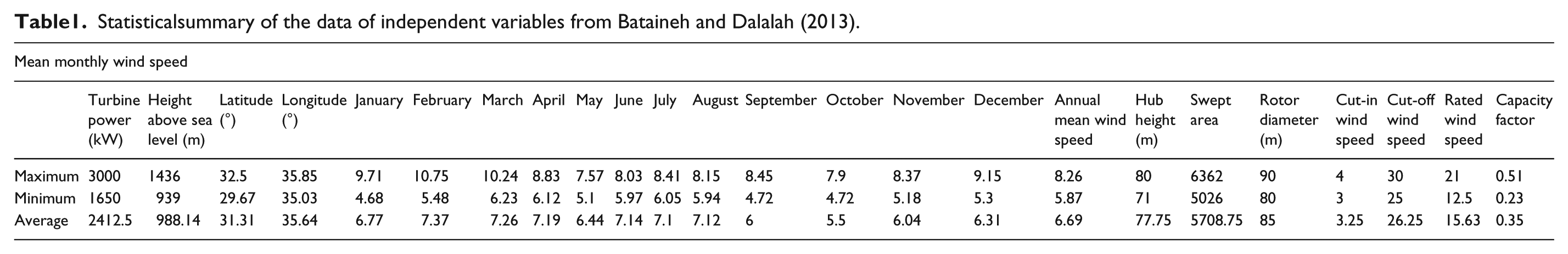
Data are obtained from the experimental investigations conducted at different stations in Jordan. The stations are Hofa, Ibrahimya, R. Monief, Zabda, Tafila, Fujaij and Aqaba. Details of these sites can be found in Bataineh and Dalalah (2013).The variables measured to characterize the wind farm stations are elevation above sea level, latitude, longitude, monthly wind speed and annual mean wind speed as well as turbine characteristics. The characteristics of different turbines together with their capacities are important parameters that can offer insight into the EV from a wind farm system. Therefore, other variables are obtained from the main characteristics of the different commercial turbines such as hub height, swept area, rotor diameter, cut-in wind speed, cut-off wind speed, rated wind speed and rated power. The different turbines utilized by Bataineh and Dalalah (2013) were Torres TWE (1.65 MW), Nordex 2.5 (2.5 MW), GE (2.5 MW) and Vestas (3 MW). The dependent or target variable is the EV. Tables 1 and 2 contain the independent and dependent data obtained from Bataineh and Dalalah (2013). This work has particular interest in these characteristics for the purpose of modelling. It also has interest in the output of such models – the EV from the different wind turbines.

Table1.

Statisticalsummary of the data of independent variables from Bataineh and Dalalah (2013).

Mean monthly wind speed
	Turbine power (kW)	Height above sea level (m)	Latitude (°)	Longitude (°)	January	February	March	April	May	June	July	August	September	October	November	December	Annual mean wind speed	Hub height (m)	Swept area	Rotor diameter (m)	Cut-in wind speed	Cut-off wind speed	Rated wind speed	Capacity factor
Maximum	3000	1436	32.5	35.85	9.71	10.75	10.24	8.83	7.57	8.03	8.41	8.15	8.45	7.9	8.37	9.15	8.26	80	6362	90	4	30	21	0.51
Minimum	1650	939	29.67	35.03	4.68	5.48	6.23	6.12	5.1	5.97	6.05	5.94	4.72	4.72	5.18	5.3	5.87	71	5026	80	3	25	12.5	0.23
Average	2412.5	988.14	31.31	35.64	6.77	7.37	7.26	7.19	6.44	7.14	7.1	7.12	6	5.5	6.04	6.31	6.69	77.75	5708.75	85	3.25	26.25	15.63	0.35

Table 2.

Statistical summary of the data of dependent variable energy gain obtained from Bataineh and Dalalah (2013).

	Energy gain (MW)
Maximum	11,101
Minimum	3944
Average	7165.43

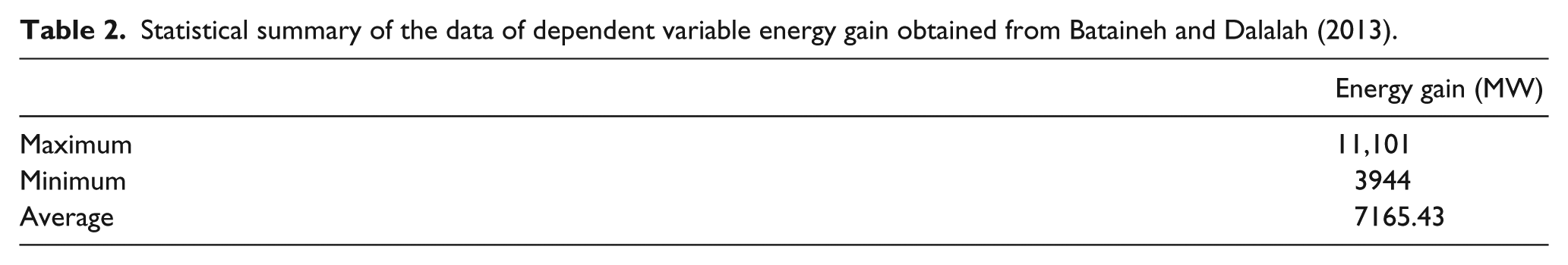
Tables 1 and 2 show the independent and dependent variables, respectively, used in training the ANN models in this work.

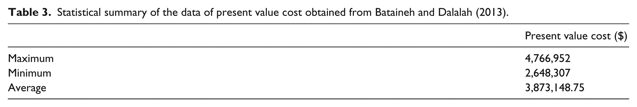
Data for cost analysis were also obtained from Bataineh and Dalalah (2013). To model the cost data, the variables in Tables 1 and 2 were used in addition to the present value cost (PVC) and project life (20 years). All data were obtained from Bataineh and Dalalah (2013). A summary of the PVC data is shown in Table 3.

Table 3.

Statistical summary of the data of present value cost obtained from Bataineh and Dalalah (2013).

	Present value cost ($)
Maximum	4,766,952
Minimum	2,648,307
Average	3,873,148.75

ANN modelling

ANN is a computational means to model a system based on known input–output data, when nothing is previously known about that system; referred to as black box. The modelling technique entails different configurations or architectures that can enhance its performance. Often, these configurations are chosen and trained by users till the desired outputs are satisfactory. Many times, the issue is approximating a static nonlinear mapping, $f (x)$ with a neural network $f_{n n} (x)$ , where $x \in ℝ^{k}$ . Multilayer perceptron (MLP) networks and the radial bass function are the most useful neural networks in function approximation.

In this work, an MLP is utilized. This network consists of an input layer, one or more hidden layers and an output layer. As mentioned earlier, ANN modelling is based on building blocks or elements called ‘neurons’, grouped into input, hidden and output layers with respective biases, weights and transfer functions. Operations involving neuron $i$ , in an MLP network are typically represented as shown in Figure 1.

Figure1.

Typical operation around a single neuron in MLP network (Wang and Fu, 2008).

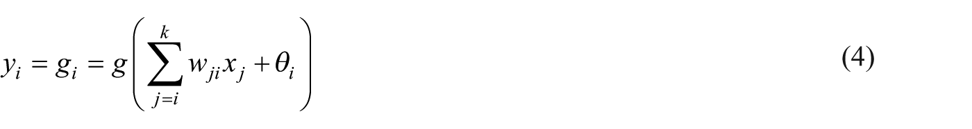
Figure 1 shows a summation (Ʃ) and a nonlinear activation or transfer function (g). The inputs to neuron $i$ are $(x_{k})$ where $k = 1, \dots, K (# o f i n p u t s)$ . The inputs are multiplied by weights $w_{k i}$ and are then summed together with a bias term $(θ_{i})$ that is a constant for each neuron. The described mathematical process results in a value $(n_{i})$ that serves as input to the activation function (g). The common activation functions in use are the hyperbolic tangent (tanh) and sigmoid function. The tanh function is expressed in equation (1) as

t a n h (x) = \frac{1 - e^{- 2 x}}{1 + e^{- 2 x}}

(1)

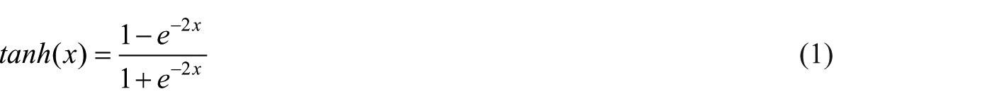
Expressions for tangent-sigmoid (tansig) and log-sigmoid (logsig) transfer functions are shown in equations (2) and (3) as

t a n s i g (x) = \frac{2}{(1 + e^{- 2 x}) - 1}

(2)

l o g s i g (x) = \frac{1}{(1 + e^{- x})}

(3)

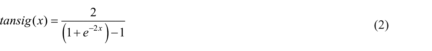
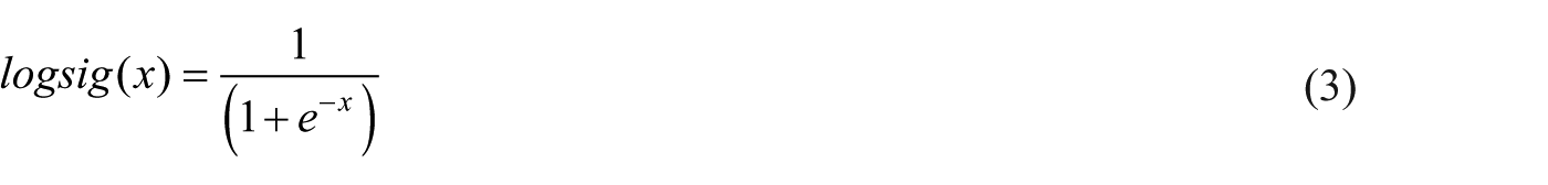
In this work, tansig transfer function is used at the hidden layer while the linear transfer function (purelin), is used at the output layer.

From Figure 1, $(y_{i})$ , the output of neuron $(i)$ after the activation function is

y_{i} = g_{i} = g (\sum_{j = i}^{k} w_{j i} x_{j} + θ_{i})

(4)

The above description illustrates the basics of ANN operation at node or neuron level. Several nodes can be connected in series or parallel to form an MLP network.

From the literature, different ANN configurations to simulate two-phase flow systems were tested by Hanspal et al.(2013). In their work (Hanspal et al., 2013), single-hidden layer and double-hidden layer ANN configurations were tested with different numbers of neurons. The results showed that both the configurations performed efficiently at different values of water saturation. Also, Abidoye and Das (2015) used different ANN configurations, with various numbers of neurons, to predict the influence of dynamic effects on two-phase flow properties. They found that a double-hidden layer MLP performs better than a single-hidden layer. However, they noticed that the differences in the predicted values by the different configurations were insignificant. Thus, it is accepted that a well-trained and validated single-layer ANN structure should suffice (Abidoye and Das, 2015; Hanspal et al., 2013).

In this work, single and double-hidden layer ANN networks are tested with two, three and four neurons in each of the layers. The configuration is represented as ANN[I-N-O}] for the single-hidden layer network, where ‘I’ represents the number of variables in the input data, ‘N’ represents number of neurons in the hidden layer and ‘O’ represents the number of variables in the output layer. For example, ANN[24-2-1] represents single-hidden layer network with 24 variables in the input, 2 neurons in the hidden layer and 1 variable in the output layer (e.g. EV). For the double-hidden layer, ANN[24-2-2-1] represents 24 variables in the input, 2 neurons in the first hidden layer and 2 neurons in the second hidden layer, then 1 variable in the output layer (e.g. EV). These configurations are chosen to test the effectiveness in predicting the energy output of a wind farm system. In line with the conclusion of Hanspal et al.(2013), the ANN structure is trained in several rounds till a satisfactory output is obtained with correlation value of at least R²~ 0.9. To implement the simulation procedure in MATLAB, program files are prepared to create, train, validate and test the network as well as generate the goodness-of-fit parameters of the data points using correlation coefficients (R²) and mean squared error (MSE). The mathematical expressions for the correlation coefficients and MSE are shown in equations (5) and (6), respectively, as

R^{2} = 1 - \frac{\sum_{i = 1}^{N} {(Y_{m e a s u r e d, i} - Y_{p r e d i c t e d, i})}^{2}}{\sum_{i = 1}^{N} {(Y_{m e a s u r e d, i} - \frac{\sum_{i = 1}^{N} Y_{m e a s u r e d, i}}{N})}^{2}}

(5)

M S E = \frac{1}{N} \sum_{i = 1}^{N} {(Y_{m e a s u r e d, i} - Y_{p r e d i c t e d, i})}^{2}

(6)

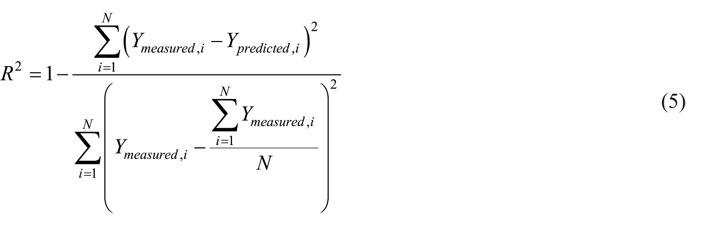
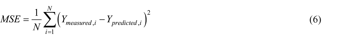
where N is the total number of data points predicted, $Y_{m e a s u r e d, i}$ is the observed or target values of the i-th EV and $Y_{p r e d i c t e d, i}$ are the predicted or calculated values of the i-th EV.

ANN modelling divides the dataset randomly into 60% for training, 20% for validation and the remaining 20% for testing. A curve-fitting function known as the Levenberg–Marquardt function is used in training the network. The function optimizes the parameters of the model curve in the nonlinear least squares problems. It uses back-propagation algorithm that consists of iterative adjustment of the weights and biases, which are used by the transfer function to relate the input layer to the hidden layer. The training process is terminated when the error between the input and the output reduces below the previously defined minimum or the number of epochs specified is attained.

As stated earlier, the (tansig) transfer function (equation (2)) is used at the hidden layers. It is a non-linear transfer function that calculates a layer’s output from its net input. MSE is used as the network default performance criterion, which relates the calculated output from the model to the actual target.

In the training process, the epochs and goals serve as the stopping criteria of the number of iterations and the error tolerance, respectively. Epoch is the maximum number of times; all the training sets are presented to the network while the goal refers to the maximum error tolerance between the predicted and the actual output. Thus, the training stops if the error goal is satisfactory or the maximum number of epochs is attained. In this work, an epoch of 200 and a goal of 0 are used. At the end of the training, network object is generated with indication of the best validation performance. The result from the training giving the best performance is then selected and the network object saved for prediction purpose. As mentioned before, criteria of the performance included R²and MSE. Thus, the network with the best performance criteria is saved for use in the prediction of the parameter sensitivity.

Nonlinear regression – XLSTAT

XLSTAT is a robust analysis software with multiple statistical add-ins for Microsoft Excel. Its packages include regression (linear, nonlinear and logistic), principal component analysis, discriminant analysis, parametric test, analysis of variance (ANOVA), and analysis of covariance (ANCOVA).

In this work, nonlinear regression is also chosen to model the wind farm data. The aim is to obtain a numerical comparison with ANN output. The better of the outputs will then be used to explore technical feasibilities of wind farm systems. The function used with the regression analysis is expressed in equation (7) as

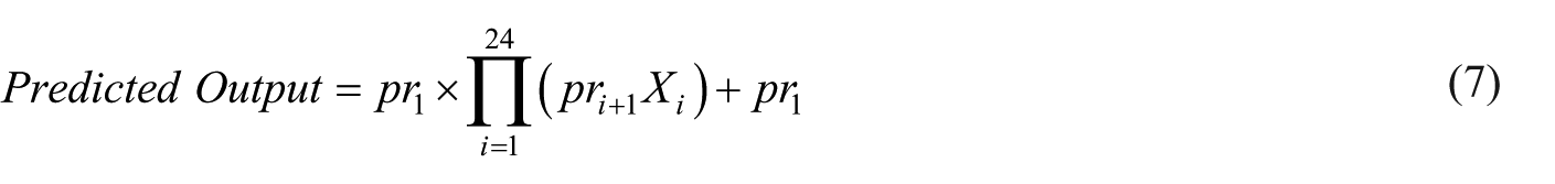
P r e d i c t e d O u t p u t = p r_{1} \times \prod_{i = 1}^{24} (p r_{i + 1} X_{i}) + p r_{1}

(7)

where $X_{i}$ is value of i-th value of variable X, $p r_{i + 1}$ is a constant value associated with variable $X_{i}$ and $\prod_{i = 1}^{24} (p r_{i + 1} X_{i}) = (p r_{2} X_{1}) (p r_{3} X_{2}) \dots (p r_{25} X_{24})$ .

The best nonlinear regression has the performance obtained in Table 4.

Table 4.

Nonlinear regression –XLSTAT performance for the energy gain.

Goodness-of-fit statistics (Y)
Observations	28.000
Sum of weights	28.000
DF	17.000
R ²	0.968
Adjusted R²	0.949
MSE	197,181.022
RMSE	444.051

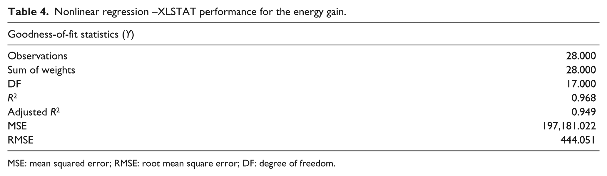
MSE: mean squared error; RMSE: root mean square error; DF: degree of freedom.

Sensitivity analysis

Sensitivity analysis was performed with the best-performing network or model from either the ANN or nonlinear regression from XLSTAT. To do this, the value of the selected independent variable was raised or lowered by some percentage. This new hypothetical value was then used to predict new EV. By comparing the new EVs from different hypothetical values of tested parameters, it can be understood how sensitive the values of the parameters to the EV are, that is, how the parameter value contributes to the amount of EV. Prediction is done using the best performing model from among the different ANN configurations and regression analysis.

The independent variables that are well correlated to the output variable are increased by 5%, 10% and/or 20%.

Results and discussions

Modelling and simulations of EV from wind farm systems were conducted for different stations in Jordan using both the ANN and XLSTAT. In addition, cost analyses of the systems were simulated. The performances of different configurations of modelling tools (ANN and linear regression) as well as the sensitivity of the output (EV) to changes in input parameters were also assessed. Discussion of the results of these investigations is presented in the following sub-sections.

Comparison of outputs from ANN and nonlinear regression

In order to ensure selection of the better computational tool, the performances of ANN and nonlinear regression were compared. Four different ANN configurations with single- and double-hidden layers were selected. In the case of the double-hidden layer networks, three configurations were tested. The first had three neurons in each of the hidden layers, the second had four and the last had two neurons in each hidden layer. For the single layer case, two neurons was used in the hidden layer. The performances of these ANN models were then compared among themselves and with that of the regression analysis.

Figure 2 shows the performance of the non-regression analysis and some ANN models. The plot in the regression analysis (Figure 2(a)) begins from the origin while those of the ANN did not (i.e. starts from 4000). As a result, it may appear that the prediction points in the regression cluster around the line of best fit more than in the ANN models. Critical analysis shows that prediction data in the regression analysis are more divergent from the line of best fit than those data from ANN models. These behaviours hint that the ANN models outperform the nonlinear regression model in predicting the output of the wind farm system. It should be noted that the x- and y-axis labels in Figure 2 refer to the predicted output data of the statistical model and data observed from the original investigations, respectively.

Figure2.

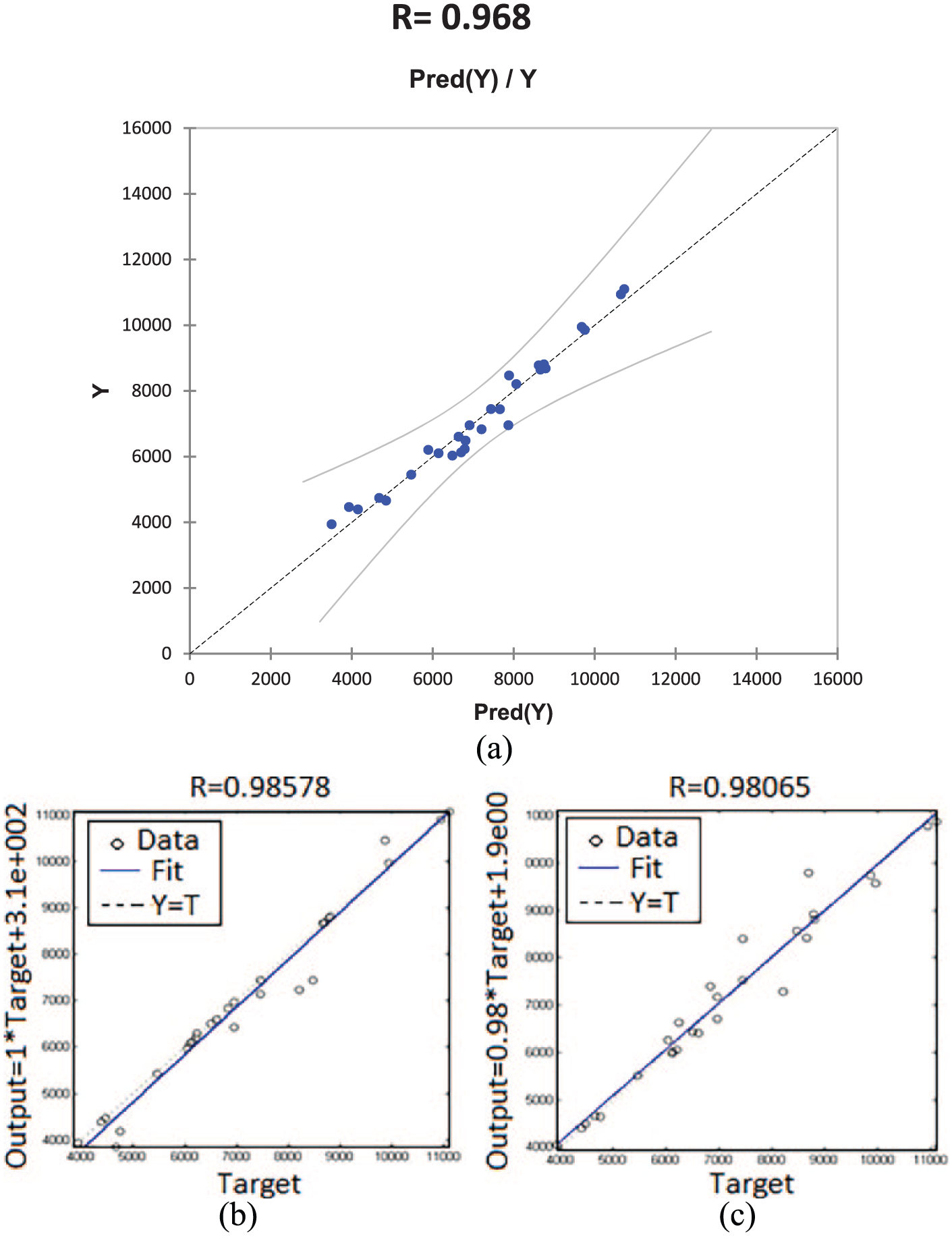
Comparison of performances of ANN and nonlinear regression models. (a) Nonlinear regression model prediction. (b) Prediction by ANN model with three neurons in each of the double-hidden layers. (c) Prediction by ANN model with four neurons in each of the double-hidden layers.

The results in Figure 2 show that ANN models are better predictors than the nonlinear regression models. From Table 4, the R² value for the regression model was 0.968. Meanwhile, from Figure 2(b) and (c), the R² values for ANN models were approximately 0.986 and 0.981, for ANN[24-3-3-1] and ANN[24-4-4-1], respectively. The value of R² describes how close the predicted value is to the original data, where higher values mean closer relation. Performance statistics are important in judging the closeness of the performance to perfection. These statistics include R² and MSE values. R² of 1 and MSE of 0 imply perfect prediction.

Therefore, it can be concluded that ANN models are more appropriate in assessing the technical feasibilities of the wind farm system.

Having concluded from the comparison in section ‘Comparison of outputs from ANN and Nonlinear Regression’ that ANN models are better suited for predicting outputs of a wind farm system, performances of the different ANN models are further analysed, in order to arrive at the best ANN configuration to be used in sensitivity analysis of wind farm parameters. As stated earlier, several rounds of training were conducted to improve learning by the ANN. Figure 3 shows the learning profiles in the training, test and validation processes, using double-hidden layer ANN configuration (ANN[24-2-2-1]). It can be seen in Figure 3(a) that regression analysis indicates good performance of the ANN model in matching the measured field data. The analysis gives very good correlation value (R > 0.99). The predicted data of EV can also be seen to cluster around the line of best fit, with most of the data points falling exactly on the line.

Figure3.

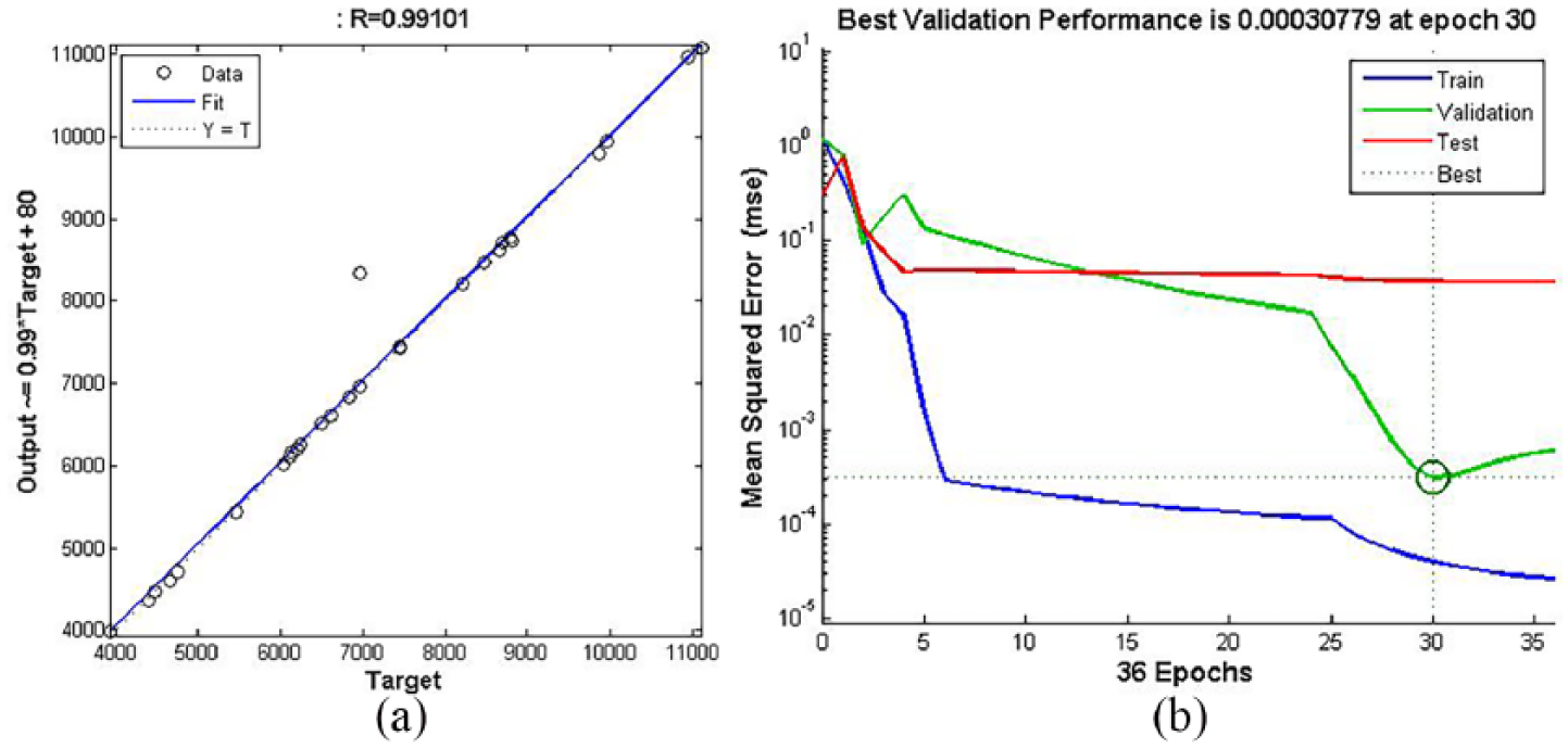
ANN modelling of energy gain, using double-hidden layer configuration (two neurons in each of the hidden layers) (ANN[24-2-2-1]). Output is the ANN prediction and Target is the original experiment data.

The outstanding results of the ANN model can be understood better with the training, validation and test processes in the procedure of ANN modelling. It can be seen from Figure 3(b) that the training process shows good learning by the network, with a fall in MSE as the number of epochs increases. The test process also shows a reduction in MSE as the number of epochs increases. The validation process follows a similar profile as earlier described and the best performance is obtained at the very low MSE value of 3.1 × 10⁻⁴at the 30th epoch. This shows that ANN can learn and approximate dependent values of a physical system after a few rounds of training, with the appropriate arrangement of input parameters.

A single-hidden layer ANN configuration with two neurons at the hidden layer is considered to further compare the performance of different ANN configurations. The training, testing, validation and regression analyses are shown in Figure 4. The profiles of the performances during different processes follow similar patterns, as described earlier for the double-hidden layer model. The regression also gives good correlation value of R ≈ 0.99. The validation process has its best performance at MSE value of approximately 2.3 × 10⁻²which occurs at the 8th epoch.

Figure4.

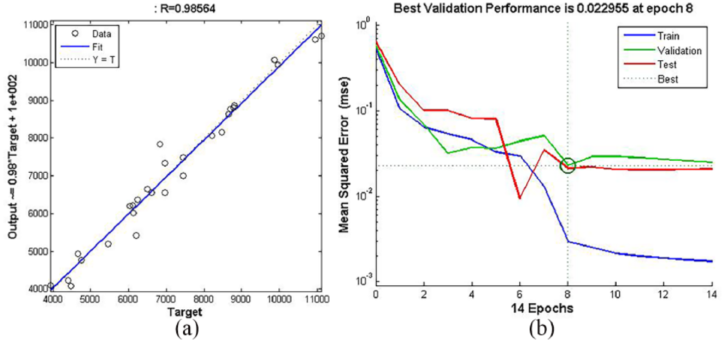
Regression and performance of ANN modelling of energy gain, using single-layer configuration (two neurons in the hidden layer) (ANN[24-2-1]). Output is the ANN prediction and Target is the original experiment data.

In comparison, the double-hidden layer ANN configuration (shown in Figure 3) displays better prediction of the EV judging from the correlation value (R) as well as the MSE for validation process. In comparison to Figure 2(b) and (c) and Figure 4, these criteria of performance (R² and MSE) have better values for the ANN[24-2-2-1]). In addition, visual observations from the figures indicate tighter clustering of data points around the line of best fit in the regression for the ANN[24-2-2-1]). Thus, judging from these results, the double-hidden layer ANN configuration ANN[24-2-2-1] shows better prediction than the other models. As a result, the prediction of EV in this work is performed using this model, with two neurons at each hidden layer.

Overall, all of the ANN models perform better at prediction, considering their high R² values (more than 0.98), in contrast to that of nonlinear regression (0.968). Also, MSE values of the ANN model ANN[24-2-2-1] (shown in Figure 3) is 3.1 x 10⁻⁴while that of regression model is outrageously high at 197181.022 (see Table 4). Therefore, ANN model with two neurons at each of the double-hidden layers performs best according to the needs of this work. It should be noted that the performance of different ANN configurations is dependent on training. This has already been reported by Hanspal et al.(2013). The ANN model with a lower number of neurons can even outperform that of higher neurons, if given sufficient training rounds.

Sensitivity analysis

After the rigorous exercise to establish the best-performing ANN model, the ANN configuration of the double-hidden layer with two neurons in each layer is chosen to predict the EV from wind farm systems based on the myriads of parameters listed in Table 1. That is, the ANN[24-2-2-1] was adjudged to have the best performance. Sensitivity analysis was performed in order to further understand the degree or level of impact on EV by individual parameter from among those listed in Table 1. That is, to know the individual impact of the selected parameter on the value of the EV. To do this, the value of the selected parameter was raised or lowered by some percentage. This new hypothetical value was then used to predict new EV. By comparing the new EVs from different hypothetical values of tested parameters, it can be understood how sensitive the values of the parameters are to the EV, that is, how the parameter value contributes to the amount of EV. The prediction is done using the best performing ANN configuration, ANN[24-2-2-1].

Statistical analysis by Bani-Hani and Abidoye (2016) showed good correlation between EV and annual mean wind speed. Good correlations are also reported between EV, rotor diameter and power. From the report in Bani-Hani and Abidoye (2016), this work takes a cue to investigate percentage contribution expected from these wind energy parameters, that is, annual mean wind speed, rotor diameter and turbine power. Figure 5 shows patterns of change of EV with various degrees of change in annual mean wind speed, at all wind stations, using a 3 MW turbine. It can be seen that at all stations, EV increases with increase in the annual mean wind speed. It is the highest at 20% increment in annual mean wind speed for each station. This is followed by 10% and 5% increment, respectively. Thus, there is a direct relationship between EV and annual mean wind speed. Proper location of wind farm along the wind route is essential for efficient energy generation. As a result of the 20% rise in annual wind speed, slightly more than 10% rise was recorded in EV at Hofa, 5% at Monief, 14.4% at Ibrahimya, 12.6% at Zabda, 12.2% at Tafila, 11.35% at Fujaji and 10.6% at Aqaba.

Figure5.

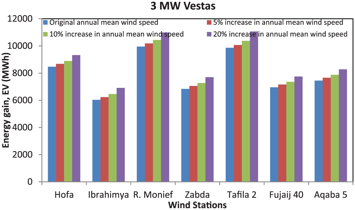
ANN modelling of energy gain at 5%, 10% and 20% increases in annual mean wind speed (3 MW turbine).

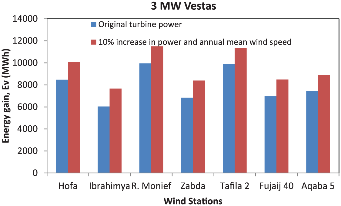
Contribution of turbine power to the eventual EV is also investigated. The results are displayed in Figure 6, which shows the relation between changes in EV and turbine power, for a 3 MW turbine. The figure shows that EV rises with increase in percentage of turbine power, while other parameters are kept constant. Therefore, EV increases as the turbine power increases at all stations. A similar pattern is observed when turbine power is increased for the 1.65 MW turbine (Figure 7), and 2.5 MW turbines from Nordexand GE, as shown in Figures 8 and 9, respectively. For the 3 MW Vestasturbine (Figure 6), more than 28% rise was recorded in EV for a 20% rise in turbine power at Hofa, 14.4% at Ibrahimya, 19.6% at Monief, 31.6% at Zabda, 16.7% at Tafila, 30.6% at Fujaji and 25.8% at Aqaba.

Figure6.

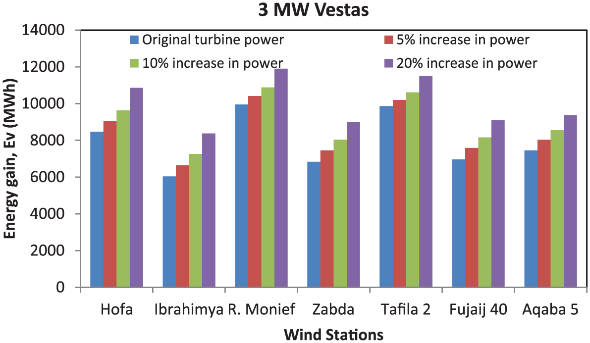
ANN modelling of energy gain with respect to increases in turbine power for the 3 MW turbine.

Figure7.

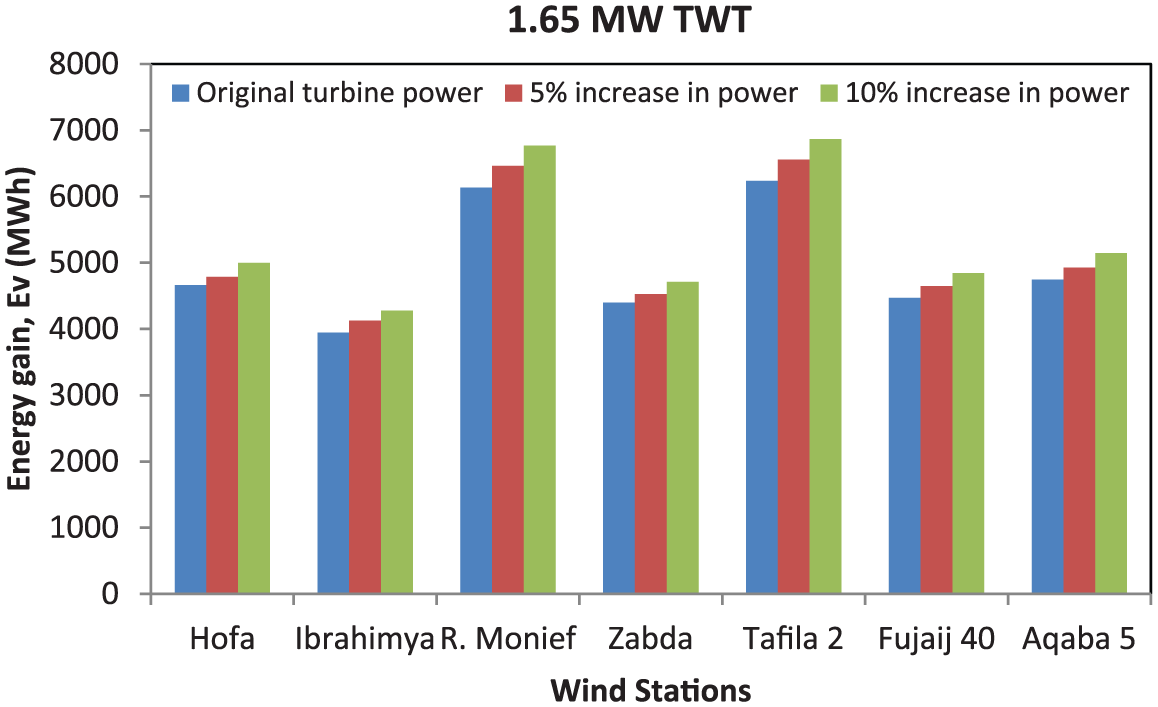
ANN modelling of energy gain with respect to increases in turbine power for the 1.65 MW turbine.

Figure8.

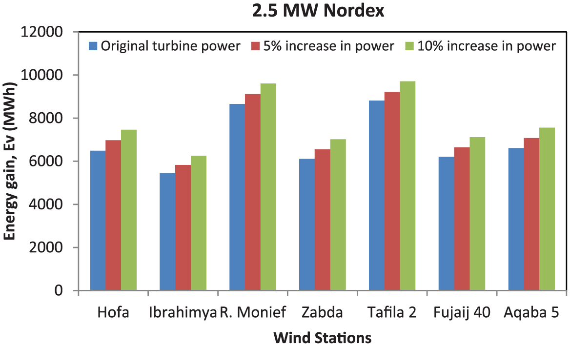
ANN modelling of energy gain with respect to increases in turbine power for the 2.5 MW Nordex turbine.

Figure9.

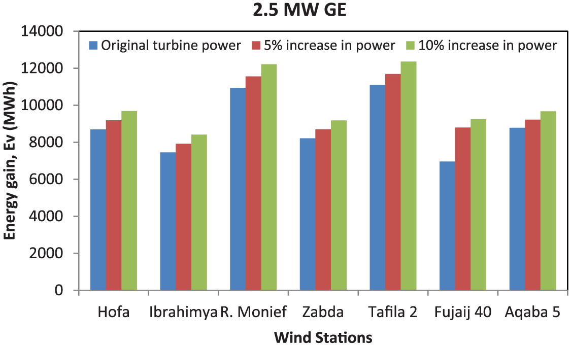
ANN modelling of energy gain with respect to increases in turbine power of the 2.5 MW GE turbine.

The above results showcase the applicability of ANN in modelling and predicting the performance of wind farm systems. It serves to identify parameters of importance that can boost EV. The implication of the above results is that EV from various wind stations is heavily dependent on wind speed and can be improved through the deployment of higher power turbines. However, it can be noticed from the figures that the increase in EV hardly exceeds 10% of the original EV. While it is necessary to locate a region of higher wind speed, the cost of procuring a new turbine with higher rated power may play a role in the most effective choice, considering the marginal EV.

ANN simulations have also been conducted for two-fold changes in wind farm performance parameters. This is realistic because practical scenarios often exhibit changes in many parameters simultaneously. We have modeled changes affecting both the turbine power and annual mean wind speed. Figure 10 shows the effect of these changes on the EV at the different wind stations. It is interesting to note that the increase in EV under two-fold changes (wind speed and turbine power) is higher than in the above cases, where only a single parameter change was simulated. However, it is noticed that the increase in EV for the two-fold change is approximately equal to the sum of the individual increments resulting from the two single-parameter cases. Assuming all other parameters are kept the same. For example, a 10% rise in annual mean wind speed at the Hofa wind station would result in approximately 5% increment in EV (please refer to Figure 5). On the other hand, a 10% rise in turbine power at the same station would result in an increment of 14% in EV (please refer to Figure 6). Modelling the two changes simultaneously resulted in an increment in EV of 19% (please refer to Figure 10).

Figure10.

ANN modelling of energy gain at 10% joint increase in turbine power and annual mean wind speed.

Furthermore, among the parameters reported with good correlation to EV is the turbine’s rotor diameter (Bani-Hani and Abidoye, 2016; Mohammadi et al 2018). The results of ANN simulations of the effect of rotor diameter on EV are shown in Figure 11. As the rotor diameter increases, there is a rise in EV. In quantitative terms, a 5% increase in rotor diameter would result in approximately 12% rise in EV. This is a greater leap in EV compared to a similar 5% increase in any of the other parameters. It is even more interesting to note that for a 10% rise in rotor diameter, there is approximately 24% increase in EV. This is more than four times higher than the EV for an equivalent change in the annual mean wind speed. It is also more than 70% higher than the effect of an equivalent change in turbine power. These results indicate that EV from a wind farm system can be enhanced using influences of both machine and environmental parameters. Machine parameters include turbine power and rotor diameter while environmental parameters include annual mean wind speed. However, simulations of the developed ANN model have identified that machine parameters contribute more to EV than environmental ones.

Figure11.

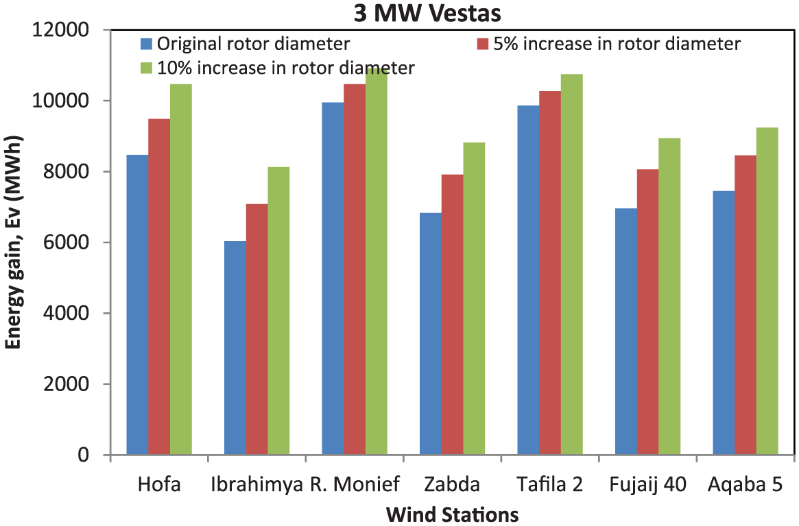
ANN modelling of energy gain at 5% and 10% increases in the rotor diameter of 3 MW turbine.

Bataineh and Dalalah (2013) performed analyses of energy cost for the sites under consideration using PVC. To evaluate the applicability of our proposed ANN model to energy cost estimation, we performed a simulated analysis on the energy cost for these sites and compared the results with those of Bataineh and Dalalah (2013).The same independent parameters used in modelling the EV were employed in modelling the energy cost. Additional parameters like PVC and machine lifetime were also included in the simulation. Figure 12 shows the ANN prediction of energy cost compared to the actual values reported in Bataineh and Dalalah (2013). It can be seen that there is an almost perfect match between the predicted and the measured values. This indicates that the developed ANN model can also be reliably applied to estimation of energy cost for wind energy systems.

Figure12.

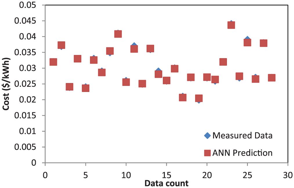
ANN prediction of measured data on energy cost.

Conclusion

A model using ANN has been presented to study the effects of various environmental and machine factors on EV from wind farm systems. It has been demonstrated that ANN is a better statistical predictor based on numerical comparison with non-linear regression. Following several rounds of training, it has been shown that the double-hidden layer ANN configuration has better performance than the single-hidden layer configuration. The developed ANN model was used to show how EV increases as a result of increases in annual mean wind speed, and the relation appears to be proportional to the percentage increment in the wind speed. The model demonstrated a similar pattern of increase in EV with respect to a modelled increase in turbine rated power across many turbine types. The model predicted that an increase in rotor diameter would result in the highest leap in EV compared to comparable changes in any of the other parameters under consideration. The model also predicted that the combined effect on EV of multiple parameter changes is equivalent to the sum of the effects of changes in individual parameters. Finally, it was demonstrated that the proposed ANN model was also a good predictor for energy cost resulting from specific wind farm design parameters. Overall, this work shows that ANN can be reliably applied in the simulation of EV and cost for wind energy systems. As an additional result from the simulations, it is observed that increasing turbine power is not a cost-effective measure to increasing EV in a wind farm since the predicated gain is less than 10% even for a 20% increase in turbine power.

Footnotes

Declaration of conflicting interests

The author(s) declared no potential conflicts of interest with respect to the research, authorship and/or publication of this article.

Funding

The author(s) received no financial support for the research, authorship and/or publication of this article.

ORCID iD

Mamdouh El Haj Assad

References

Abidoye

Bello

(2017) Simple dielectric mixing model in the monitoring of CO2 leakage from geological storage aquifer. Geophysical Journal International 208(3): 1787–1795.

Abidoye

Das

(2015) Artificial neural network modeling of scale-dependent dynamic capillary pressure effects in two-phase flow in porous media. Journal of Hydroinformatics 17(3): 446–461.

Abidoye

Mahdi

(2014) Novel linear and nonlinear equations for the higher heating values of municipal solid wastes and the implications of carbon to energy ratios. Journal of Energy Technologies and Policy 4(5): 14–27.

Abidoye

Wairagu

(2013) Simulation of oil spill infiltration and redistribution in a shallow aquifer. Academic Journals 7(6): 546–554.

Acker

Williams

Duque

, et al. (2007) Windresource assessment in the state of Arizona: Inventory, capacity factor, and cost. Renewable Energy 32: 1453–1466.

Alghoul

Sulaiman

Azmi

, et al. (2007) Wind energy potential of Jordan. International Energy Journal 8: 71–78.

Amato

López

Peña-Méndez

, et al. (2013) Artificial neural networks in medical diagnosis. Journal of Applied Biomedicine 11(2): 47–58.

Ammari

Al-Rwashdeh

Al-Najideen

(2014) Evaluation of wind energy potential and electricity generation at five locations in Jordan. Sustainable Cities and Society 15: 135–143.

Anani

Zuamot

Abu-Allan

, et al. (1998) Evaluation of wind energy as a power generation source in selected sites in Jordan. Solar & Wind 5(1): 64–67.

10.

Bani-Hani

Abidoye

(2016) Prediction of energy gains from Jordanian wind stations using artificial neural network. International Journal of Energy and Environmental Research 4(1): 26–41.

11.

Bataineh

Dalalah

(2013) Assessment of wind energy potential for selected areas in Jordan. Renewable Energy 59: 75–81.

12.

Das

Gill

Abidoye

, et al. (2014) A numerical study of dynamiccapillary pressure effect for supercritical carbon dioxide-water flow in porousdomain. Aiche Journal 60(12): 4266–4278.

13.

Habali

Hamdan

Jubran

, et al. (1987) Wind speed and wind energy potential of Jordan. Solar Energy 38(1): 59–70.

14.

Hanspal

Allison

Deka

, et al. (2013) Artificial neural network (ANN) modeling of dynamic effects on two-phase flow in homogenous porous media. Journal of Hydroinformatics 15(2): 540–554.

15.

Kalogirou

(1999) Applications of artificial neural-networks for energy systems. Applied Energy 40(10): 17–35.

16.

Khashei

Bijari

(2014) Fuzzy artificial neural network (p, d, q) model for incomplete financial time series forecasting. Journal of Intelligent and Fuzzy Systems 26(2): 831–845.

17.

Mohammadi

Lakestani

Mohamed

(2018) Intelligent parameter optimization of Savonius rotor using artificial neural network and genetic algorithm. Energy 143: 56–68.

18.

Mueller

Hemond

(2013) Extended artificial neural networks: Incorporation of a priori chemical knowledge enables use of ion selective electrodes for in-situ measurement of ions at environmentally relevant levels. Talanta 117: 112–118.

19.

Muyeen

Hasanien

Al-Durra

(2014) Transient stability enhancement of wind farms connected to a multi-machine power system by using an adaptive ANN-controlled SMES. Energy Conversion and Management 78: 412–420.

20.

Petković

Arif

Shamshirband

, et al. (2015) Sensorless estimation of wind speed by soft computing methodologies: A comparative study. Informatica 26(3): 1–16.

21.

Spalding

(1981) A general purpose computer program for multi-dimensional one-and two-phase flow. Mathematics and Computers in Simulation 23(3): 267–276.

22.

Wang

(2008)Artificial Neural Networks. Hoboken,NJ:Wiley.

23.

White

(1989) Learning in artificial neural networks: A statistical perspective. Neural Computation 1(4): 425–464.

24.

Widrow

(1962) Generalization and information storage in networks of adaline neurons. In: Jovitz

Jacobi

Goldstein

(eds) Self-Organizing Systems. Washington, DC: Spartan Books,pp. 435–461.

25.

Yurdakul

Akdas

(2013) Modeling uniaxial compressive strength of building stones using non-destructive test results as neural networks input parameters. Construction and Building Materials 47: 1010–1019.

26.

Zhang

Eddy Patuwo

(1998) Forecasting with artificial neural networks. International Journal of Forecasting 14(1): 35–62.