Application of Realistic Artificial Data for Testing Various Crash Safety Analyses: A Case Study for Rural Two-Lane Undivided Highways

Abstract

Traffic safety research will continue to create new and improved methods for the analysis of safety data. Even if these models perform well, the precise underlying crash mechanism remains unknown. The missing piece is a tool that may be used to evaluate how well a method identifies the cause-and-effect relationship in the data. To meet these safety analysis needs, a high-resolution disaggregate data generating process called realistic artificial data (RAD) was developed. This tool simulates crash incidence on transportation facilities, capturing real-world causal links between individual roadway characteristics and crashes. The objective of this study was to check if the stochasticity embedded in the RAD generation process will be consistent for different random seeds and miles of data generated from the tool. To accomplish this, 10 different datasets were generated from the RAD tool and estimated using the negative binomial model; parameter estimates from the model were checked using a revised Wald statistic. The t-statistic estimates showed that the differences among the parameter values across the dataset are within a statistically acceptable level. Given the stability of the tool, the RAD framework can be useful in addressing the known limitations and knowledge gap in assessing the extent to which a statistical method succeeds in identifying the cause-and-effect relationship in the data. This in return can help guide and improve the practical application of statistical methods and eventually lead to more effective safety countermeasures that can reduce highway-related injuries and fatalities.

Keywords

data and data science statistical methods safety performance and analysis crash data crash prediction models highway safety manual

Every year, approximately 1.3 million people’s lives are cut short as a result of highway crashes. Additionally, between 20 and 50 million people suffer non-fatal injuries, with many of them resulting in disability ( 1 ). The entire economic cost of fatal and non-fatal preventable incidents in 2020 was over 1 billion dollars, including vehicle damage, lost wages and productivity, and medical expenses ( 2 ). Because of the enormous societal costs associated with these crashes, research for many decades has focused on developing qualitative and quantitative information on how to make roads safer ( 3 ). Despite the strides made in the direction of the societal goal of Vision Zero through targeted legislation and the implementation of relevant safety-related measures, much work remains to be done in the field of safety analysis ( 4 ).

The goal of any traffic safety analysis is to identify and quantify the influence of factors contributing to the occurrence of traffic crashes and their associated consequences. Highway safety crash data have long been used to analyze safety problems, with uses ranging from identification of safety problems to determining their extent and creating models that are used to predict crashes ( 5 ). Even though the availability of safety crash data overall has expanded over the years, this does not necessarily mean that the quality of crash data is keeping up with the methodological advances ( 4 ). Earlier studies have tended to concentrate on the modeling component of the entire crash prediction process by developing new modeling approaches that offer superior fit, and the acquired data is implicitly believed to be a sufficient representation of reality.

Traditional statistical methods use archived safety data to guide the development of a model functional form, which is then used to estimate coefficients for variables, identify and compare significant factors, and finally compare which statistical method is best suited for a given scenario ( 6 ). Even if a model performs well, it may not accurately represent or identify the cause-and-effect relationship, because the intention of any developed model is prediction rather than identifying causal factors. Unfortunately, the detailed driving data and crash data that would better enable identification of cause-and-effect relationships in crash probabilities are typically not available ( 7 ). Most researchers have addressed this problem by framing their analytic approaches to study the factors that affect the number of crashes occurring on a roadway segment or intersection over some specified period.

Small sample size, time interval variation, and temporal and spatial autocorrelation are some of the most well-documented model estimation issues that have been raised in the literature ( 8 ). These problems are a potential source of error in modeling crash data that may cause incorrect estimates and inferences. Crash data, as previously mentioned in the literature ( 7 , 9 –12), are frequently characterized by a sparse number of observations which can produce a low sample mean. This characteristic is attributed to the possibility that crash data for some roadway entities may include few observed crashes which results in a preponderance of zeros. Although it is believed that the size of the sample will have an impact on the crash prediction model’s performance, some have suggested a rule of thumb for data size requirements ( 7 , 8 , 10 ). A study reported that the dispersion parameter of Poisson-gamma models estimated from data characterized by low sample mean values and small sample size can be significantly biased (the value is likely to be mis-estimated) and negatively affect analyses commonly performed in highway safety ( 8 ). There is a significant increase in the probability that the dispersion parameter cannot be reliably estimated when the sample mean and sample size decrease.

The issue of time interval variance in crash data was also reported by other studies ( 7 , 10 ). Crash data are often collected over a certain time period. Over the collection period, some explanatory variables and their relationship to the crash incidents may change, a reality that is not usually considered because of the lack of detailed data within the collection period ( 10 ). Ignoring within-period variation in explanatory variables may result in biased estimation of parameters and incorrect prediction of crashes as a result of unobserved heterogeneity.

While the continuing march of methodological innovation has increased our understanding of the factors that affect crash frequencies, the potential of integrating improving methodology with significantly more detailed crash data offers the most promise for the future ( 3 ). To meet these safety analysis needs, a high-resolution disaggregate data generating process called realistic artificial data (RAD) was developed, which simulates crash incidence on transportation facilities. The tool was created to capture the real-world causal link between individual route parameters and crash statistics. The crash counts from the tool will be based on a set of (secret) “causal rules” that represent predetermined correlations between crash frequency/severity and specific roadway geometric characteristics ( 4 ).

Since the data generation process is now known, the RAD can serve as a testbed which will help us determine whether a statistical model developed indeed captures the underlying relationship between the independent variables and the resultant crashes, and this in turn will help guide and improve the practical application of statistical methods that will influence highway safety policy and eventually lead to more effective safety countermeasures that can reduce highway-related injuries and fatalities. In addition, there are many other questions which the RAD can help us answer, such as how many mile-years of data are necessary to produce valid results when a large amount of data is available.

The purpose of this study is to examine the stability of the parameters from different datasets generated from a RAD tool. The tool as stated earlier is a combination of a roadway generator and a crash generator with a predetermined causal relationship between roadway descriptors and crash frequency and severity. Estimation of crash prediction models for rural two-lane undivided highway segments was selected as a case study. Ten different datasets—two sets each of 150, 300, 500, 750, and 1000 mi—with different random seeds were generated from the tool. Negative binomial (NB) models were estimated with each of the datasets generated. Then we employed revised Wald statistics on the parameter estimates from the models to determine whether the estimates were stable across the different generated datasets. Examining the stability of the multiple datasets generated is important so we know that the randomness embedded in the RAD generation process is reliable.

Previous Work

The idea of RAD for traffic safety is not new; the early conception can be traced back to Dr Ezra Hauer who presented this idea at a 2008 TRB workshop titled “Future Directions in Highway Crash Data Modeling” ( 6 ). In a project funded by FHWA, Council et al. ( 13 ) investigated the effectiveness of various modeling approaches for cross-sectional studies. Highway Safety Information System (HSIS) data from Washington State were used to construct a dataset with 2400 mi of homogeneous segments that were each 0.02 mi long. They looked at single-vehicle lane-departure crashes on two-lane roadways. A modeler who was not aware of the presumed causal relationships was then given the crash and roadway data. The goal of the modeler was to estimate regression models and identify the causal relationships. The model’s outcomes were then compared with the assumed relationships. Another study by Lan and Srinivasan ( 14 ) utilized datasets produced by RAD for rural two-lane roads to examine the effectiveness of various regression models for calculating the crash modification factor (CMF) of horizontal curvature. To achieve this, three volunteers without prior knowledge of the embedded safety relationship used the RAD to estimate CMFs for horizontal curvature. This comparison was conducted for different levels of annual average daily traffic (AADT) and terrain. The CMFs estimated by the volunteers were then compared with the embedded safety relationship between horizontal curvature and crashes within the RAD. Horizontal curve radii that were higher rather than lower generally resulted in estimated CMFs that were closer to the true CMF values. Models that used site characteristics apart from AADT and curve radius usually performed better.

Miaou ( 15 ) studied the relationship between highway geometric characteristics and crashes using NB regression. Miaou suggested that the Poisson regression model should be used to establish the relationship between highway geometry and crashes. If overdispersion exists and is found to be moderate or high, the NB model can be explored. Another study by Abdel-Aty and Radwan ( 16 ) used NB modeling to model the frequency of crash occurrence, showing that high traffic volume, speeding, narrow shoulder width, and narrow lane width increase the likelihood of a crash. Some variations of count models have also been developed, such as zero-inflated NB models.

Anastasopoulos and Mannering ( 17 ) explored the use of random parameter count models as another methodological alternative in analyzing accident frequencies. Their findings showed that ignoring the possibility of random parameters when estimating count-data models can result in substantially different marginal effects and subsequent inferences relating to the magnitude of the effect of factors on accident frequencies. Shankar et al. ( 18 ) suggest that simple Poisson and NB modeling efforts do not address the possibility that some roadway sections observed to have no accidents during a specified time period may be qualitatively different from Poisson- or NB-distributed accident frequency counts.

A study by Malyshkina et al. ( 19 ) proposed a two-state Markov switching count-data model as an alternative to zero-inflated models to account for the preponderance of zeros sometimes observed in transportation count data. They proposed to overcome some of the criticism associated with the zero-accident state of the zero-inflated model by allowing individual roadway segments to switch between zero and normal-count states over time. They showed that the Markov switching model is a viable alternative and results in a superior statistical fit relative to the zero-inflated models. However, Lord et al. ( 20 ) in their study provided defensible guidance on how to appropriate model crash data. They suggested that carefully selecting the time/space scales for analysis, including an improved set of explanatory variables and unobserved heterogeneity effects in count regression models, or applying small-area statistical methods (observations with low exposure) represent the most defensible modeling approaches for datasets with a preponderance of zeros.

Other models that have been applied to crash frequency analysis based on their strength include multivariate models, which can model different crash types simultaneously ( 21 , 22 ); Poisson-lognormal models, which are more flexible than Poisson-gamma at handling overdispersion ( 23 , 24 ); and a generalized estimating equation for its ability to handle temporal correlation ( 25 – 27 ).

A Brief Overview of the RAD Generation Process

RAD Generation Process

The roadway generator and crash data generator are the two parts of the RAD framework used in this work. The roadway generator generates homogeneous segments with realistic road characteristics that represent variables typically found in the inventories of state transportation agencies. The Markov chain Monte Carlo principle is used in the road generator to assign specific values for the road characteristics. Markov chain is a systematic method for generating a sequence of random variables for which the current value is probabilistically dependent on the value of the prior variable. Specifically, selecting the next variable is only dependent on the last variable in the chain. The assignment characteristics of the developed roadway generator incorporate various Markov chain transition tables that determine probabilities of a descriptor changing based on data from various states ( 4 ). A random variable indicating how well the roadway characteristics change based on segment length according to the type of facility was also incorporated into the framework. That is, if you are trying to assign the shoulder width on a given segment, it has some high probability of being the same as the preceding segment but there is also some low probability that it will change.

The crash data generator is embedded with secret causal rules defining the true relationship between roadway descriptors and crash frequency and severities, that is, specifying how each roadway descriptor will affect a given crash type. Crash counts by crash type and severity are generated using well-known model structures and realistic relationships between crash counts and roadway characteristics; with this process, randomness in crashes per segment is generated for each user’s data ( 4 ). A system then combines the roadway and crash generator, producing a roadway file that attaches crash counts to each segment. The overall framework for generating the RAD is presented in the flow chart shown in Figure 1.

The RAD generation tool is in the form of a database stand-alone software application that can be customized and run to prepare multiple realizations of data for various facility types under different random seeds and dataset specifications, such as total dataset mileage, using various combinations of inputs. This tool will be owned and operated by an entity where researchers who have no knowledge of the safety relationships that were embedded into the system can compare the results from their analysis. The degree to which they succeed will then be made evident by having the entity that owns the RAD generator compare the estimated parameters to the known relationships embedded in the data. The tool will serve as a testbed to help determine whether a statistical model indeed captures the underlying cause-and-effect relationship.

Crash Model Estimation Method

Although different mixed-Poisson distributions have been developed to model crash data (e.g., Poisson-lognormal, Poisson-inverse Gaussian, etc.), the most common distribution used for modeling crash data remains the Poisson-gamma, aka the NB distribution. The NB distribution offers a simple way to accommodate the overdispersion, especially since the final equation has a closed form and the mathematics to manipulate the relationship between the mean and the variance structures is relatively simple ( 12 ). The NB/Poisson-gamma model assumes that the Poisson parameter follows a gamma probability distribution. The model results in a closed-form equation and the mathematics to manipulate the relationship between the mean and the variance structures is relatively simple. The NB model is derived by rewriting the Poisson parameter for each observation i as

λ_{i} = EXP (β X_{i} + ε_{i})

(1)

where EXP ( $ε$ _i) is a gamma-distributed error term with mean 1 and variance α. The addition of this term allows the variance to differ from the mean as VAR[y_i] = E[y_i][1 + αE[y_i]] = E[y_i] + αE[y_i]. The Poisson regression model is a limiting model of the NB regression model as α approaches zero, which means that the selection between these two models is dependent on the value of α. The parameter α is often referred to as the overdispersion parameter.

Data Generation

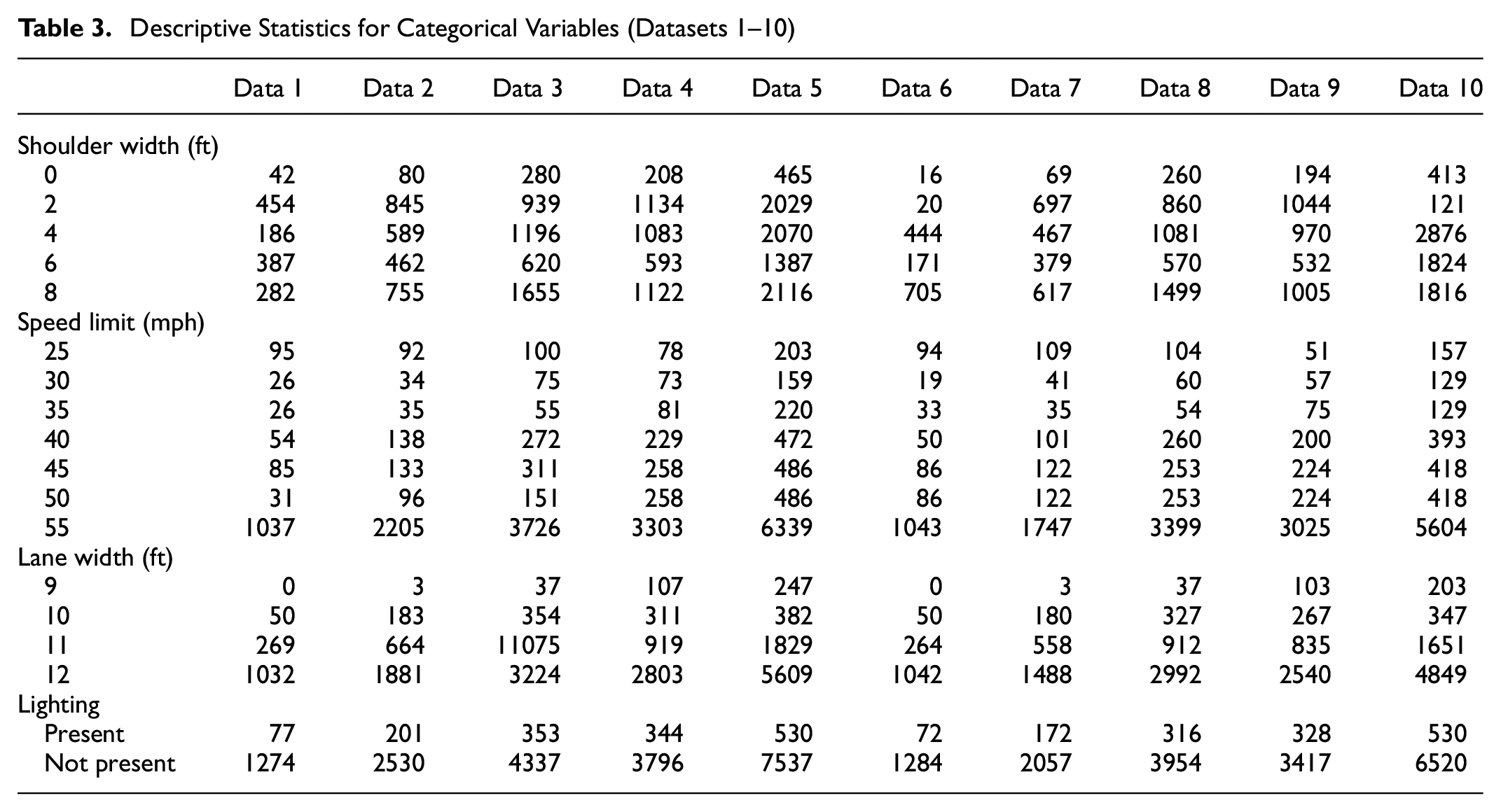
The data for the analysis was drawn from the RAD tool. The two-lane undivided roadway data contained horizontal curve data, crash data, and roadway data as described in Tables 1 to 3. To accomplish the objective of this study, all that was needed was to generate several RADs differing in mile-years of data and then to run various statistical models on all the datasets with the goal of showing the stability of the parameters from the dataset generated from the tool by examining the differences between the estimated and the assumed parameter values. Only the NB model for total crashes will be illustrated in this study because of space limitations. Ten different datasets—two sets each of 150, 300, 500, 750, 1000 mi—with different random seeds were generated. It should be noted that the same sized dataset (e.g., the two sets of 150 mi) resulted in different numbers of observations because of the data being randomly generated. In addition, the roadway characteristics generated had the same distribution as the sample size increase, which is a result of the effects described by the central limit theorem.

Table 1.

Descriptive Statistics for Continuous Variables (Datasets 1–5)

Continuous variables	Data 1 (n = 1351) 150 mi		Data 2 (n = 2742) 300 mi		Data 3 (n = 4690) 500 mi		Data 4 (n = 4140) 750 mi		Data 5 (n = 8667) 1000 mi
Continuous variables	Mean	SD	Mean	SD	Mean	SD	Mean	SD	Mean	SD
Crash counts PDO	0.938	1.752	0.856	1.615	0.853	1.684	1.231	2.52	0.95	1.80
Crash counts K	0.005	0.094	0.003	0.060	0.005	0.092	0.007	0.150	0.004	0.088
Crash counts A	0.168	0.565	0.137	0.477	0.143	0.504	0.223	0.765	0.168	0.583
Crash counts B	0.041	0.247	0.041	0.241	0.047	0.278	0.060	0.374	0.057	0.323
Crash counts C	0.157	0.454	0.165	0.493	0.158	0.486	0.282	0.908	0.193	0.552
Pavement roughness	104	34.04	104.5	34.656	105.3	40.64	107.6	40.30	105.9	39.800
Pavement condition	40.170	3.090	39.85	3.077	23.0	3.714	39.37	3.791	39.33	3.730
Average superelevation	0.769	2.603	0.769	2.586	−8.00	2.576	−8.183	11.94	−19.61	9.240
Curvature degree	4.320	8.435	5.217	10.354	5.21	9.30	0.00	4.750	5.52	10.91
Arc angle	36.53	20.62	35.16	21.904	10.0	22.08	43.29	12.42	36	22.670
Log(radius)	7.686	0.904	7.189	0.943	7.17	0.830	8.281	0.842	7.153	0.920
Log segment length	−2.710	1.066	−2.72	1.058	−2.75	1.056	−2.383	1.22	−2.63	1.101
Vertical approach	0.225	0.828	0.293	0.910	0.355	0.895	0.504	1.094	0.44	0.960
Vertical leaving	0.239	0.873	0.213	0.822	0.221	0.831	0.340	1.017	0.26	0.930
Log(AADT)	7.735	0.570	7.394	0.845	7.628	0.832	7.381	0.851	7.56	0.804
Grade	0.353	1.075	0.402	1.090	0.462	1.080	0.671	1.30	0.56	1.170

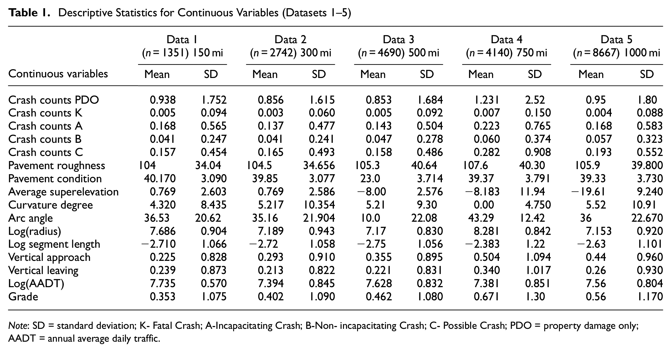
Note: SD = standard deviation; K- Fatal Crash; A-Incapacitating Crash; B-Non- incapacitating Crash; C- Possible Crash; PDO = property damage only; AADT = annual average daily traffic.

Table 2.

Descriptive Statistics for Continuous Variables (Datasets 6–10)

Continuous variables	Data 6 (n = 1361) 150 mi		Data 7 (n = 2229) 300 mi		Data 8 (n = 4270) 500 mi		Data 9 (n = 3749) 750 mi		Data 10 (n = 7050) 1000 mi
Continuous variables	Mean	SD	Mean	SD	Mean	SD	Mean	SD	Mean	SD
Crash counts PDO	0.870	1.751	0.988	1.997	0.923	1.841	1.432	2.751	1.087	2.13
Crash counts K	0.0044	0.085	0.0085	0.232	0.0014	0.037	0.008	0.230	0.0079	0.27
Crash counts A	0.153	0.561	0.156	0.536	0.165	0.629	0.247	0.855	0.167	0.63
Crash counts B	0.036	0.234	0.052	0.306	0.054	0.336	0.073	0.386	0.064	0.370
Crash counts C	0.196	0.527	0.213	0.613	0.186	0.618	0.397	0.810	0.219	0.641
Pavement roughness	104.7	33.54	104.9	34.96	105.1	39.29	108.5	40.83	106.7	40.7
Pavement condition	40.28	3.173	39.63	3.18	39.59	3.76	39.4	3.728	39.24	3.70
Average superelevation	0.802	2.60	0.771	2.608	0.737	2.59	−9.14	12.14	−19.07	9.74
Curvature degree	5.155	10.17	4.624	8.563	5.062	8.943	3.122	2.970	5.367	10.27
Arc angle	36.06	22.72	40.75	18.904	37.79	19.92	45.33	5.557	37.41	20.93
Log(radius)	7.143	0.931	7.694	1.094	7.463	1.051	8.657	0.304	7.397	1.034
Log segment length	−2.69	1.053	−2.58	1.126	−2.69	1.087	−2.29	1.249	−2.576	1.150
Vertical approach	0.2323	0.850	0.316	0.950	0.361	0.913	0.548	1.134	0.459	0.990
Vertical leaving	0.252	0.905	0.250	0.874	0.236	0.848	0.369	1.055	0.277	0.936
Log(AADT)	7.739	0.575	7.411	0.858	7.616	0.835	7.357	0.891	7.542	0.820
Grade	0.370	1.05	0.446	1.145	0.4741	1.104	0.728	1.35	0.594	1.200

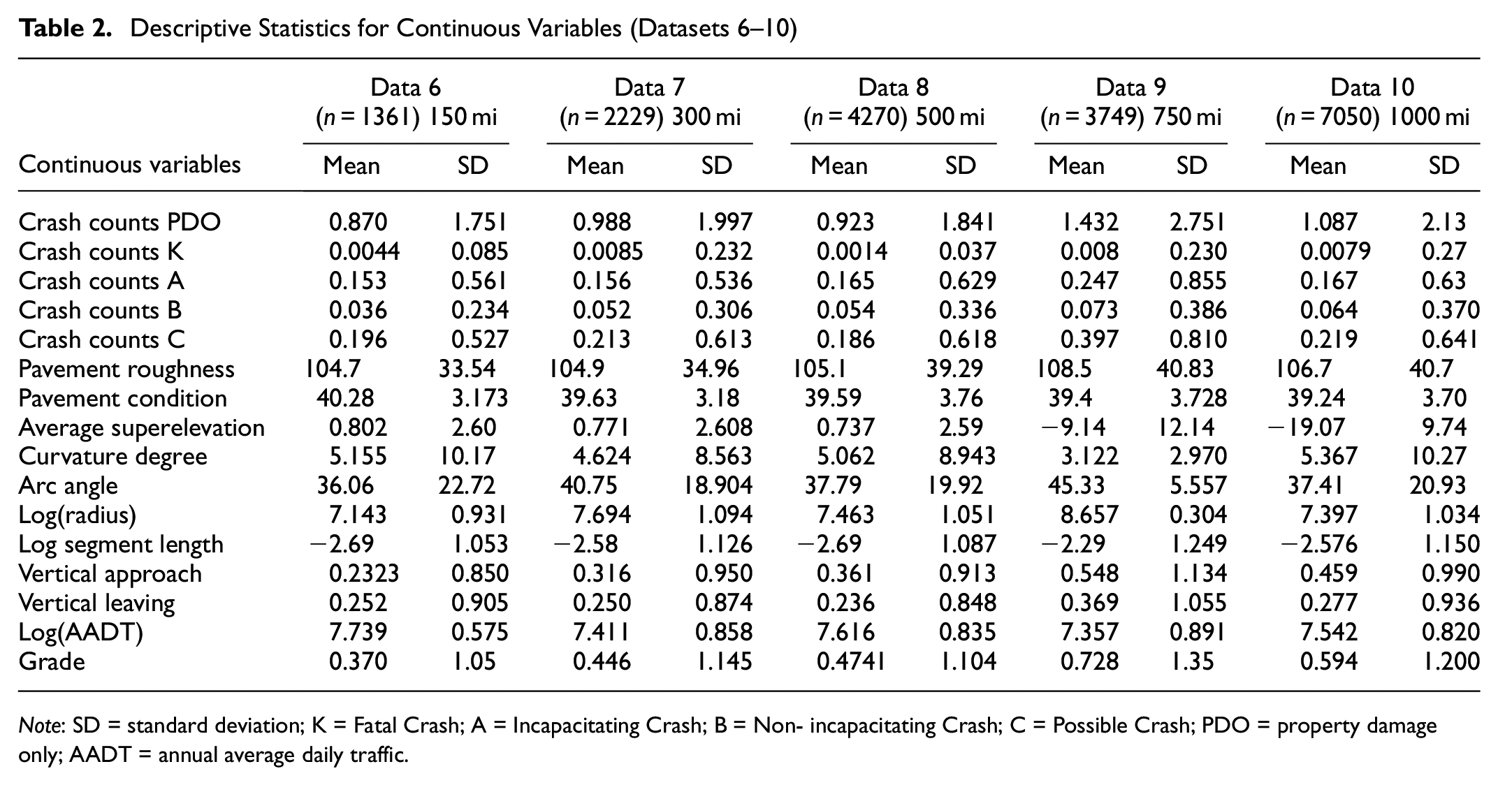
Note: SD = standard deviation; K = Fatal Crash; A = Incapacitating Crash; B = Non- incapacitating Crash; C = Possible Crash; PDO = property damage only; AADT = annual average daily traffic.

Table 3.

Descriptive Statistics for Categorical Variables (Datasets 1–10)

	Data 1	Data 2	Data 3	Data 4	Data 5	Data 6	Data 7	Data 8	Data 9	Data 10
Shoulder width (ft)
0	42	80	280	208	465	16	69	260	194	413
2	454	845	939	1134	2029	20	697	860	1044	121
4	186	589	1196	1083	2070	444	467	1081	970	2876
6	387	462	620	593	1387	171	379	570	532	1824
8	282	755	1655	1122	2116	705	617	1499	1005	1816
Speed limit (mph)
25	95	92	100	78	203	94	109	104	51	157
30	26	34	75	73	159	19	41	60	57	129
35	26	35	55	81	220	33	35	54	75	129
40	54	138	272	229	472	50	101	260	200	393
45	85	133	311	258	486	86	122	253	224	418
50	31	96	151	258	486	86	122	253	224	418
55	1037	2205	3726	3303	6339	1043	1747	3399	3025	5604
Lane width (ft)
9	0	3	37	107	247	0	3	37	103	203
10	50	183	354	311	382	50	180	327	267	347
11	269	664	11075	919	1829	264	558	912	835	1651
12	1032	1881	3224	2803	5609	1042	1488	2992	2540	4849
Lighting
Present	77	201	353	344	530	72	172	316	328	530
Not present	1274	2530	4337	3796	7537	1284	2057	3954	3417	6520

Empirical Analysis

An NB regression model was estimated for each dataset. The objective was to check whether the stochasticity embedded in the RAD generation process will be consistent for different random seed of data generated from the tool. To achieve this, the parameter estimate from the NB models for each dataset was examined using the revised Wald test statistics created by Hoover et al. ( 28 ) as shown below.

Parameter test statistics = abs [\frac{sample parameter - population benchmark}{\sqrt{SE sampl e^{2}} - \sqrt{SE populatio n^{2}}}]

(2)

To check the differences in the parameters across the datasets, the t-statistics for all the parameters across all the datasets samples were computed using the computation of the test statistic mentioned above. Dataset 10 (1000 mi) was used as the benchmark to evaluate whether the parameters for other datasets were statistically different relative to this sample dataset. If the parameter test statistic is greater than the 90% t-statistic, it indicates that there is a significant difference between the datasets. On the other hand, if the parameter test statistics is below the 90% t-statistic, there is no significant difference between the datasets, and we can trust that the stochasticity in the RAD tool is consistent across different generations with different random seeds.

Model Results

Table 4 shows the NB parameter estimates for total crashes for all 10 databases. A visual examination reveals that the parameter estimates for each dataset model are relatively close to one another. Comparing the estimated parameters requires having the same variables in all models; to balance variable significance with identical variable sets, we dropped variables that were statistically insignificant based on the 90% significance level in more than six datasets. It was noted that the majority of the categories for lane width and speed limit in datasets 1 and 6 were statistically insignificant at 90% significance level; nonetheless, these variables were left in because the parameter estimate was rather logical in comparison with what has been published in other literature. Overall, the parameter estimates are consistent with what would normally be obtained when using conventional crash data, showing that the RAD tool generates data with reasonable relationships among the variables. However, the main objective of the study was focused on checking for parameter stability across the datasets with different random seeds and varying sizes generated using the tool.

Table 4.

Negative Binomial Estimates for Total Crashes

Parameter	Data 1	Data 2	Data 3	Data 4	Data 5	Data 6	Data 7	Data 8	Data 9	Data 10
Intercept	−0.621^a (0.860)^b	−3.870 (0.685)	−1.856 (0.369)	−2.001 (0.389)	−1.965 0.291	−1.000* (1.176)	−3.278 (0.671)	−1.917 (0.448)	−2.438 (0.385)	−2.223 (0.321)
Ln(length)	0.963 (0.036)	1.054 (0.034)	1.023 (0.021)	1.058 (0.019)	1.049 (0.017)	0.965 (0.050)	1.050 (0.031)	1.074 (0.025)	1.048 (0.021)	1.064 (0.017)
Ln(AADT)	0.392 (0.065)	0.627 (0.045)	0.548 (0.027)	0.452 (0.025)	0.474 (0.023)	0.415 (0.089)	0.533 (0.044)	0.464 (0.032)	0.530 (0.043)	0.546 (0.088)
Shoulder width: 8 ft base level
<2 ft	0.167 (0.329)	0.610 (0.155)	0.381 (0.076)	0.240 (0.093)	0.349 (0.071)	0.818 (0.365)	0.334 (0.159)	0.266 (0.093)	0.189 (0.095)	0.246 (0.076)
>=2 ft <4 ft	0.361 (0.092)	0.497 (0.077)	0.360 (0.051)	0.292 (0.050)	0.383 (0.043)	0.781 (0.373)	0.471 (0.076)	0.249 (0.061)	0.341 (0.051)	0.329 (0.118)
>=4 ft <6 ft	0.144 (0.083)	0.446 (0.083)	0.277 (0.048)	0.257 ( 0.051)	0.243 (0.042)	0.361 (0.095)	0.410 (0.083)	0.218 (0.058)	0.307 (0.051)	0.351 (0.094)
>=6 ft <8 ft	0.168 (0.096)	0.479 (0.089)	0.137 (0.058)	0.246 (0.059)	0.217 (0.048)	0.117* (0.136)	0.332 (0.088)	0.126 (0.070)	0.177 (0.060)	0.287 (0.044)
Lane width: 12 ft base level
9 ft or less	NA	0.932 (1.071)	0.326 (0.196)	0.5047 (0.129)	0.415 (0.112)	NA	0.599* (1.088)	0.566 (0.232)	0.403 (0.130)	0.235 (0.117)
9.5–10.5 ft	0.210* (0.208)	0.252 (0.143)	0.125 (0.089)	0.256 (0.094)	0.289 (0.081)	−0.151* (0.285)	0.255 (0.142)	0.184 (0.111)	0.268 (0.093)	0.152 (0.084)
11–11.5 ft	0.008* (0.101)	0.116 (0.086)	0.183 (0.051)	0.091 (0.052)	0.141 (0.043)	0.047* (0.142)	0.374 (0.083)	0.102* (0.064)	0.152 (0.051)	0.210 (0.043)
Speed limit: 45 mph base level
25 mph	0.475 (0.062)	0.140 (0.188)	0.439 (0.116)	0.041 (0.030)	0.606 (0.102)	0.291 (0.125)	0.429 (0.174)	0.519* (0.140)	0.244 (0.139)	0.483 (0.098)
30 mph	0.171* (0.242)	0.428 (0.244)	0.210 (0.136)	0.041 (0.035)	0.349 (0.110)	0.313 (0.173)	0.385* (0.241)	−0.059* (0.184)	0.234 (0.139)	0.035* (0.111)
35 mph	−0.840* (0.271)	−0.701 (0.306)	−0.271 (0.174)	−0.295 (0.143)	0.069* (0.109)	0.268* (0.343)	−0.045* (0.253)	−0.567 0.237	−0.222 (0.150)	−0.336 (0.112)
40 mph	−0.956 (0.252)	−0.824 (0.197)	−0.822 (0.114)	−1.109 (0.119)	−0.655 (0.099)	−0.879 (0.319)	−0.992 (0.216)	−0.916* 0.144	−0.969 (0.123)	−1.021 (0.103)
50 mph	0.120* (0.233)	0.095 (0.172)	−0.163 (0.122)	0.003* (0.119)	−0.087 (0.124)	−0.425* (0.367)	−0.036 (0.178)	0.117* 0.139	−0.057 (0.130)	−0.115 (0.116)
55 mph	−0.280* (0.132)	−0.332 (0.118)	−0.254 (0.072)	−0.329 (0.071)	−0.011* (0.067)	−0.196 (0.180)	−0.066 (0.115)	−0.226 (0.089)	−0.125 (0.074)	−0.270 (0.064)
Presence of lighting	−0.341 (0.184)	−0.603 (0.151)	−0.523 (0.151)	−0.531 (0.101)	−0.412 (0.085)	−0.300 (0.259)	−0.334 (0.026)	−0.658 (0.122)	−0.306 (0.098)	−0.431 (0.085)
Presence of horizontal curve	0.549* (0.239)	0.294* (0.205)	0.078* (0.116)	0.186 (0.112)	0.264 (0.088)	0.269* (0.244)	0.407 (0.036)	0.652 (0.111)	0.168* (0.112)	0.365 (0.085)
Overdispersion	0.257	0.463	0.344	0.199	0.375	0.725	0.271	0.447	0.216	0.307
AIC	3417.6	5603.7	11292	9304.8	17328	2980.1	8947.1	4638.1	9028.3	15389
Log-likelihood	−1690.3	−2772.84	−5616.7	−4623.4	−8634.9	−1462.0	−4444.5	−2290.0	−4485.1	−7665.6

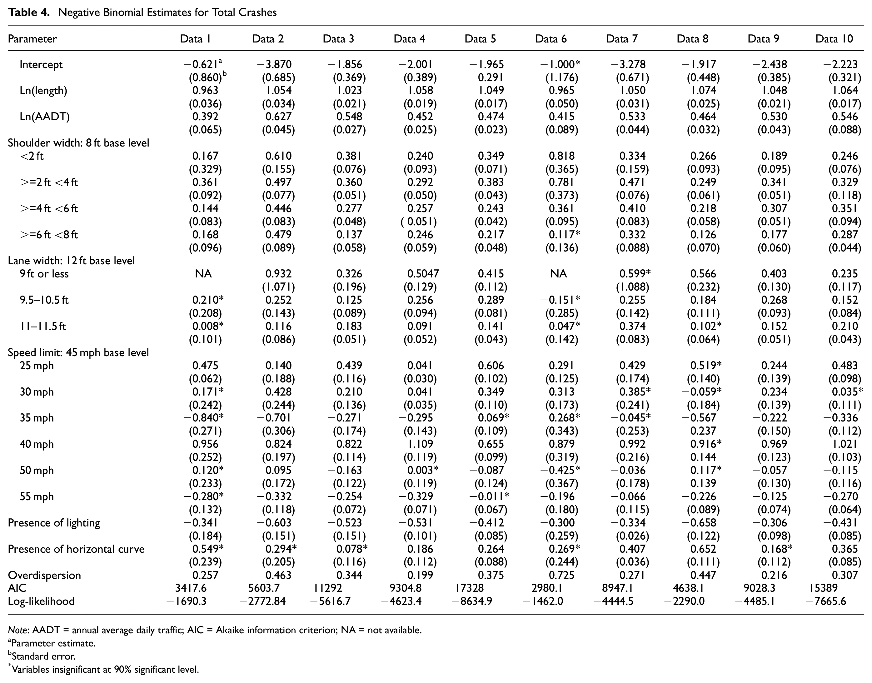
Note: AADT = annual average daily traffic; AIC = Akaike information criterion; NA = not available.

Parameter estimate.

Standard error.

Variables insignificant at 90% significant level.

Dataset 10 (1000 mi) was used as the population benchmark to evaluate whether each parameter in any model was statistically different from the corresponding one in that dataset. Dataset 10 was used because it had the largest number of observations and was believed to be the most able to produce convincing parameter estimates. As previously mentioned, if the parameter test statistic computed is higher than the 90% t-statistic, the result would indicate significant difference between the corresponding dataset and dataset 10.

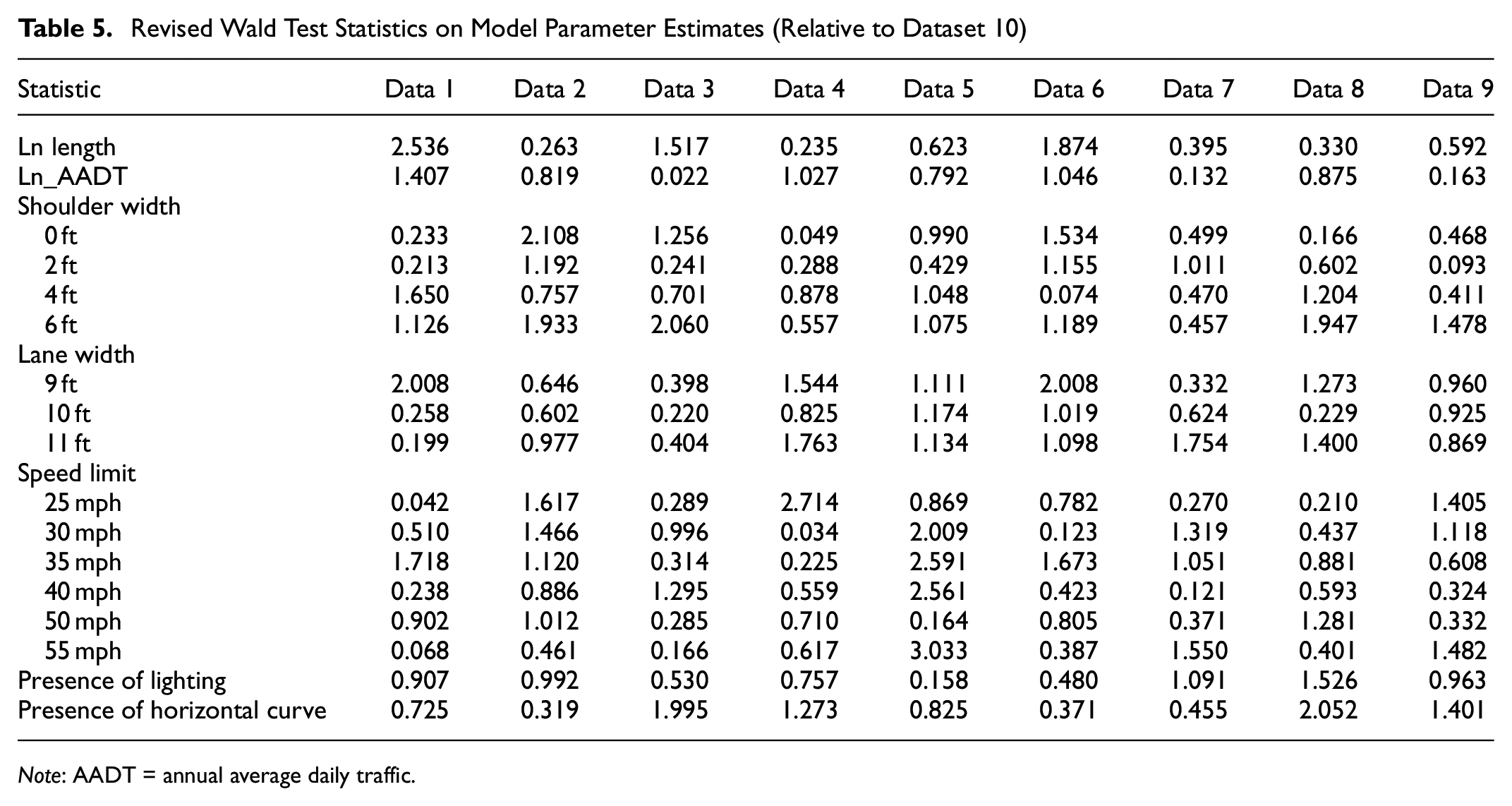
Table 5 shows the revised Wald test statistics on the model parameter estimates. The test statistics for segment length across the datasets were lower than the 90% confidence value of 1.65, which could mean that there is no significant difference between the estimated parameters in the corresponding dataset and dataset 10. The test statistics across the datasets for the AADT parameter were also lower than the 90% confidence value of 1.65, indicating that the variation across the different datasets is within a statistically acceptable level. Note that the test statistics for some of the speed limit category coefficients (i.e., 30 mph, 35 mph, and 55 mph) in dataset 6 exceeded the 90% confidence value, which might indicate that the parameter values for those categories could be significantly different relative to dataset 10. The possible reason for this could be that these parameter estimates were actually statistically insignificant on their own.

Table 5.

Revised Wald Test Statistics on Model Parameter Estimates (Relative to Dataset 10)

Statistic	Data 1	Data 2	Data 3	Data 4	Data 5	Data 6	Data 7	Data 8	Data 9
Ln length	2.536	0.263	1.517	0.235	0.623	1.874	0.395	0.330	0.592
Ln_AADT	1.407	0.819	0.022	1.027	0.792	1.046	0.132	0.875	0.163
Shoulder width
0 ft	0.233	2.108	1.256	0.049	0.990	1.534	0.499	0.166	0.468
2 ft	0.213	1.192	0.241	0.288	0.429	1.155	1.011	0.602	0.093
4 ft	1.650	0.757	0.701	0.878	1.048	0.074	0.470	1.204	0.411
6 ft	1.126	1.933	2.060	0.557	1.075	1.189	0.457	1.947	1.478
Lane width
9 ft	2.008	0.646	0.398	1.544	1.111	2.008	0.332	1.273	0.960
10 ft	0.258	0.602	0.220	0.825	1.174	1.019	0.624	0.229	0.925
11 ft	0.199	0.977	0.404	1.763	1.134	1.098	1.754	1.400	0.869
Speed limit
25 mph	0.042	1.617	0.289	2.714	0.869	0.782	0.270	0.210	1.405
30 mph	0.510	1.466	0.996	0.034	2.009	0.123	1.319	0.437	1.118
35 mph	1.718	1.120	0.314	0.225	2.591	1.673	1.051	0.881	0.608
40 mph	0.238	0.886	1.295	0.559	2.561	0.423	0.121	0.593	0.324
50 mph	0.902	1.012	0.285	0.710	0.164	0.805	0.371	1.281	0.332
55 mph	0.068	0.461	0.166	0.617	3.033	0.387	1.550	0.401	1.482
Presence of lighting	0.907	0.992	0.530	0.757	0.158	0.480	1.091	1.526	0.963
Presence of horizontal curve	0.725	0.319	1.995	1.273	0.825	0.371	0.455	2.052	1.401

Note: AADT = annual average daily traffic.

Figures 2 to 4 show the boxplot summary of the test statistics variation for parameter estimates across the datasets. The figures clearly reveal that the range of the test statistics across all the parameters is quite narrow and does not exceed the 90% confidence value of 1.65 from the parameters discussed above. In Figure 2, segment length and shoulder width (6 ft) have a majority of t-statistics falling above the upper quartile (right skewed) but still reasonably within the test of 90% significance which supports the discussion above; the parameter estimate of the other datasets relative to dataset 10 is not statistically different. The plot in Figure 3 shows the t-statistics all falling below the lower quartile (left skewed) and within the test of 90% confidence value. Figure 4 shows the variability among the various category levels of speed limit, with the test statistics all falling below the lower quartile except for speed limit (55 mph). Overall, there was variability across the different variables, but they all reasonably fall within the chosen confidence value.

Discussion

The parameter coefficients estimated using data from the tool are comparable with the estimates reached in previous studies for the variables included in this paper. For example, a study by Gooch et al. ( 29 ) quantified the safety performance of horizontal curves on two-way two-lane rural roads and estimated an AADT coefficient for total crashes as 0.697. Other studies ( 21 , 30 ) estimated 0.622 and 0.656, respectively, these estimates being comparable with the range of AADT estimates from this study. Segment length had estimates of 0.889, 0.801, and 0.459 respectively ( 27 , 29 , 31 ) while the presence of horizontal curve had estimates of 0.053 and 0.050 ( 24 , 29 ). Overall, these estimates compared with ours show that the data from the tool can produce results comparable to those from the traditional data.

Practical Implications

The results from this paper could have significant implications for highway safety research, for the development of information that can be used to make roads safer and crashes less severe. Since the data generation process in the tool is completely known it will allow objective evaluation and validation of various safety analysis methods used to verify various assumptions related to safety performance and in turn lead to providing effective countermeasures to address crashes. The RAD can also be helpful in generating large datasets with consistent conditions in cases where we cannot go back many years because of changes in road characteristics or drivers; this makes it easier to estimate models for unusual and rare events like minor crashes. In addition to this, the tool can help determine sample sizes by determining the quantity of data necessary to produce convincing results.

Conclusions

The current research uses datasets generated from the RAD tool with the objective of assessing the stability of the resulting estimated parameters across the varying datasets and random seeds. Revised Wald test statistics were generated to check whether the variation across the different datasets is within a statistically acceptable level using dataset 10 as the benchmark. The result clearly highlights the stability in various parameter estimates across the datasets.

The resulting stability found across the datasets indicates that the parameter estimates using RAD will be consistent regardless of the miles of segment-related data generated using the tool. Having this knowledge of stability, the dataset from the RAD tool can be used for other possible purposes, such as estimating different prediction models or comparing the performance of various safety analysis methods, and can also help determine the adequate sample size to get convincing results especially for fatal crashes with low realizations. This study contributes to safety research by providing data that can be used by researchers who have no knowledge of the cause–effect structure and who would apply the method they wish to assess. The degree to which they succeed would then be made evident by having the entity which owns the RAD generator compare the estimated parameters to the known relationships embedded in the data. In the future, other statistical models that have been employed by researchers, such as Poisson regression, Poisson-lognormal, random parameters, and multivariate modeling, will be used on the RAD dataset for all roadway facility types including segments and intersections, roadway specifically included in the highway safety manual.

Footnotes

Author Contributions

The authors confirm contribution to the paper as follows: study conception and design: John Ivan, Shanshan Zhao, Naveen Eluru, and Kai Wang; data collection: Oluwaseun Olufowobi, John Ivan; analysis and interpretation of results: Oluwaseun Olufowobi, John Ivan; draft manuscript preparation: John Ivan, Shanshan Zhao, and Kai Wang. All authors reviewed the results and approved the final version of the manuscript.

Declaration of Conflicting Interests

The author(s) declared no potential conflicts of interest with respect to the research, authorship, and/or publication of this article.

Funding

The author(s) disclosed receipt of the following financial support for the research, authorship, and/or publication of this article: The authors would like to gratefully acknowledge FHWA’s sponsorship in this research under project number 693JJ31950017.

ORCID iDs

John Ivan

Naveen Eluru

The ideas expressed in this work do not necessarily indicate acceptance by FHWA of the findings and conclusions expressed within.

References

Road Traffic Injuries . World Health Organization. June 21, 2021. https://www.who.int/news-room/fact-sheets/detail/road-traffic-injuries. Accessed April 15, 2022.

“Motor Vehicles.” National Safety Council, injuryfacts.nsc.org/work/costs/work-injury-costs. Accessed January 8, 2022.

Mannering

Bhat

Analytic Methods in Accident Research: Methodological Frontier and Future Directions. Analytic Methods in Accident Research, Vol. 1, 2014, pp. 1–22.

Zhao

W. S.

Wang

Eluru

Abdel-Aty

Development and Application of a Disaggregate Artificial Realistic Data Generator for Computationally Testing Safety Analysis Methods. Report No. FHWA-PROJ-19-0014. Proposal to the U.S. Department of Transportation, Federal Highway Administration, Washington, D.C., 2018.

“Safety Data and Analysis.” Federal Highway Administration, Washington, D.C., highways.dot.gov/research/research-programs/safety/safety-data-analysis. Accessed September 8, 2022.

Bonneson

Ivan

Theory, Explanation and Prediction in Road Safety. E-Circular E-C179. Transportation Research Board, Washington, D.C., 2013.

Lord

Mannering

The Statistical Analysis of Crash-Frequency Data: A Review and Assessment of Methodological Alternatives. Transportation Research Part A: Policy and Practice, Vol. 44, No. 5, 2010, pp. 291–305.

Lord

Modeling Motor Vehicle Crashes Using Poisson-Gamma Models: Examining the Effects of Low Sample Mean Values and Small Sample Size on the Estimation of the Fixed Dispersion Parameter. Accident Analysis & Prevention, Vol. 38, No. 4, 2006, pp. 751–766.

Lord

Bonneson

J. A.

Calibration of Predictive Models for Estimating the Safety of Ramp Design Configurations. Transportation Research Record: Journal of the Transportation Research Board, 2005. 1908: 88–95.

10.

Abdulhafedh

. “Road Traffic Data Crash Data: An Overview on Sources, Problems, and Collection Methods.”Journal of Transportation Technologies, Vol. 7, No. 2, 2017, pp. 206–219.

11.

Park

B.-J.

Lord

Hart

J. D.

Bias Properties of Bayesian Statistics in Finite Mixture of Negative Binomial Regression Models in Crash Data Analysis. Accident Analysis & Prevention, Vol. 42, No. 2, 2010, pp. 741–749.

12.

Lord

Miranda-Moreno

L. F.

Effects of Low Sample Mean Values and Small Sample Size on the Estimation of the Fixed Dispersion Parameter of Poisson-Gamma Models for Modeling Motor Vehicle Crashes: A Bayesian Perspective. Safety Science, Vol. 46, No. 5, 2008, pp. 751–770.

13.

Council

Hauer

Lan

Harwood

Srinivasan

Use of Artificial Realistic Data (ARD) to Assess the Performance of Cross-Sectional Analysis Methods in Capturing Causal Relationships between Individual Roadway Attributes and Safety, 2017.

14.

Lan

Srinivasan

Estimation of Crash Modification Factors with Cross-Sectional Data: An Investigation Using a Simulated Realistic Artificial Dataset. Proc., Road Safety and Simulation Conference, Iowa City, October 2019.

15.

Miaou

S.-P.

The Relationship between Truck Accidents and Geometric Design of Road Sections: Poisson versus Negative Binomial Regressions. Accident Analysis & Prevention, Vol. 26, No. 4, 1994, pp. 471–482.

16.

Abdel-Aty

M. A.

Radwan

A. E.

Modeling Traffic Accident Occurrence and Involvement. Accident Analysis & Prevention, Vol. 32, No. 5, 2000, pp. 633–642.

17.

Anastasopoulos

P. C.

Mannering

F. L.

A Note on Modeling Vehicle Accident Frequencies with Random Parameters Count Models. Accident Analysis & Prevention, Vol. 41, No. 1, 2009, pp. 153–159.

18.

Shankar

Milton

Mannering

F. L.

Modeling Accident Frequency as Zero-Altered Probability Processes: An Empirical Inquiry. Accident Analysis & Prevention, Vol. 29, No. 6, 1997, pp. 829–837.

19.

Malyshkina

N. V.

Mannering

F. L.

Tarko

A. P.

Markov Switching Negative Binomial Models: An Application to Vehicle Accident Frequencies. Accident Analysis & Prevention, Vol. 41, No. 2, 2009, pp. 217–226.

20.

Lord

Washington

S. P.

Ivan

J. N.

Poisson, Poisson-Gamma and Zero Inflated Regression Models of Motor Vehicle Crashes: Balancing Statistical Fit and Theory. Accident Analysis & Prevention, Vol. 37, No. 1, 2005, pp. 35–46.

21.

Miaou

S.-P.

Lord

Modeling Traffic Crash-Flow Relationships for Intersections: Dispersion Parameter, Functional Form, and Bayes versus Empirical Bayes Methods. Transportation Research Record: Journal of the Transportation Research Board, 2003. 1840: 31–40.

22.

Pendyala

R. M.

Washington

S. P.

Konduri

A Simultaneous Equations Model of Crash Frequency by Collision Type for Rural Intersections. Safety Science, Vol. 47, No. 3, 2003, pp. 443–452.

23.

Khan

Bill

A. R.

Chitturi

Noyce

D. A.

Horizontal Curves, Signs, and Safety. Transportation Research Record: Journal of the Transportation Research Board, 2012. 2279: 124–131.

24.

Miaou

S.-P.

Song

J. J.

Bayesian Ranking of Sites for Engineering Safety Improvements: Decision Parameter, Treatability Concept, Statistical Criterion, and Spatial Dependence. Accident Analysis & Prevention, Vol. 37, No. 4, 2005, pp. 699–720.

25.

Mohammadi

M. A.

Samaranayake

V. A.

Bham

G. H.

Crash Frequency Modeling Using Negative Binomial Models: An Application of Generalized Estimating Equation to Longitudinal Data. Analytic Methods in Accident Research, Vol. 2, 2014, pp. 52–69.

26.

Lord

Persaud

B. N.

Accident Prediction Models with and without Trend: Application of the Generalized Estimating Equations Procedure. Transportation Research Record: Journal of the Transportation Research Board, 2000. 1717: 102–108.

27.

Schneider

Zimmerman

Van Boxel

Vavilikolanu

Bayesian Analysis of the Effect of Horizontal Curvature on Truck Crashes Using Training and Validation Data Sets. Transportation Research Record: Journal of the Transportation Research Board, 2009. 2096: 41–46.

28.

Hoover

Bhowmik

Yasmin

Eluru

Understanding Crash Risk Using a Multi-Level Random Parameter Binary Logit Model: Application to Naturalistic Driving Study Data. Transportation Research Record: Journal of the Transportation Research Board, 2022. 2676: 1–9.

29.

Gooch

J. P.

Gayah

V. V.

Donnell

E. T.

Quantifying the Safety Effects of Horizontal Curves on Two-Way, Two-Lane Rural Roads. Accident Analysis & Prevention, Vol. 92, 2016, pp. 71–81.

30.

Gayah

V. V.

Donnell

E. T.

Estimating Safety Performance Functions for Two-Lane Rural Roads Using an Alternative Functional Form for Traffic Volume. Accident Analysis & Prevention, Vol. 157, 2021, p. 106173.

31.

Schneider IV

W. H.

Savolainen

P. T.

Moore

D. N.

Effects of Horizontal Curvature on Single-Vehicle Motorcycle Crashes along Rural Two-Lane Highways. Transportation Research Record: Journal of the Transportation Research Board, 2010. 2194: 91–98.