A Simple Yet Efficient K-Nearest Neighbor-Based Method for High-Resolution Traffic Time

Abstract

A time–space diagram (TSD) is an efficient tool for traffic analysis and visualization, representing the macroscopic traffic state as a set of cells. However, its application is often hampered by data sparsity, which obscures high-resolution traffic dynamics. This study proposes a modified K-nearest neighbors method, characterized by an adaptive iterative process, to impute missing TSD data. To support the method’s design, analytical bounds on error propagation motivated by Green’s function-based theory are established, and a practical empirical formula for the optimal K parameter is derived. The framework’s performance was rigorously validated on diverse data sets from China (Ubiquitous Traffic Eyes), the US (Next Generation Simulation), and Germany (HighD) across 30 distinct experimental conditions. Compared against four baseline models, the proposed model demonstrates a compelling balance between high imputation accuracy and exceptional computational efficiency. Further analyses confirm the influence of neighborhood order and the systematic performance bias. The model’s potential for knowledge transfer is also demonstrated via a cross-data set imputation scheme.

Keywords

traffic time–space diagram K-nearest neighbors traffic data imputation traffic dynamics traffic state analysis

Introduction

The time–space diagram (TSD) is a fundamental tool in transportation research, offering a visual representation of macroscopic changes in traffic flow across spatial and temporal dimensions ( 1 ). By illustrating congestion patterns, peak periods, and overall traffic trends, TSDs enable engineers and managers to analyze the dynamic characteristics of road traffic. Consequently, they are extensively applied in the study of traffic flow theory, vehicle behavior, and traffic wave propagation, advancing traffic science ( 2 – 5 ). The data populating a TSD, which represent traffic states within discrete cells, are typically sourced from fixed detectors or probe vehicles ( 6 ). However, both sources present significant limitations. Fixed detectors incur high installation and maintenance costs, resulting in low deployment density. In contrast, probe vehicles, often limited to specific fleets such as taxis, exhibit low penetration rates ( 7 ). These constraints collectively lead to data sparsity, yielding TSDs that are often insufficient to accurately represent the underlying traffic dynamics.

Existing methods mainly fall into two categories: (1) interpolation and (2) prediction ( 7 ). Interpolation techniques leverage temporal proximity or pattern similarity to estimate missing values as the average or a weighted average of adjacent data points ( 8 ). A conventional method, for instance, imputes a missing value using historical data from the same detector at a corresponding time ( 9 ). However, the efficacy of these methods hinges on the assumption of similarity between neighboring traffic states, rendering them unreliable in scenarios with contiguous missing data, a condition known as high sparsity ( 10 ). This limitation has spurred a more direct focus on the TSD problem, which moves beyond simple interpolation by attempting to model the underlying spatiotemporal relationships to reconstruct a complete, high-resolution TSD from the inputs of low-resolution TSDs. This refinement task is distinct from pure prediction because it can utilize data from all available dimensions, including temporally future data, to inform the imputation of a missing cell. A recent and important example of this approach is the work by He ( 4 ), who proposed a simple yet effective multivariate linear regression (MLR) model that leverages local spatiotemporal features to enhance the TSD resolution, establishing an important methodological baseline specifically for this refinement task.

Alongside these model-based refinement techniques, other data-driven approaches, often adapted from the broader field of traffic state estimation (TSE), have gained prominence ( 7 ). These include statistical models and, more recently, deep learning (DL). The DL techniques excel at modeling the intricate, nonlinear dependencies inherent in large-scale data sets ( 4 , 11 , 12 ). For instance, Zhang et al. ( 7 ) utilized a traffic state reconstruction generative adversarial network (TSR-GAN) to reconstruct spatiotemporal traffic states, and Xu et al. ( 13 ) proposed a multi-directional recurrent graph convolutional network to reconstruct TSDs from sparse data. These advanced DL models can achieve high imputation accuracy; however, their practical application faces significant challenges. Crucially, the TSD imputation task differs fundamentally from traditional TSE ( 14 ) because imputation can leverage future traffic states as input to enhance quality, a feature typically unavailable in real time TSEs ( 4 ). Therefore, models trained on fixed-dimension historical data may be ill-suited for the dynamic nature of TSD imputation. Furthermore, the high computational cost, extensive parameter counts, and limited transferability of complex DL models hinder their practical application in many real time intelligent transportation systems (ITS) ( 15 ).

This landscape creates a pressing need for a method capable of directly imputing TSD data that balances imputation accuracy with computational efficiency, requires minimal training data, and offers robust performance, particularly under high data sparsity. The K-nearest neighbors (KNN) algorithm presents a compelling alternative for traffic data imputation. It operates by identifying temporal or spatial neighbors based on a defined distance metric to impute missing values ( 16 – 19 ). The simplicity and efficiency of KNNs have led to their widespread application in traffic prediction and imputation ( 20 ). Notable adaptations include the Linearly Sewing Principle Component (KNN-LSPC) algorithm ( 16 ), a data-driven car-following model ( 21 ), a kernel-based KNN ( 22 ), and a hybrid model fusing KNN with support vector regression ( 17 ). A significant advantage of KNNs over more complex data-driven models is their parsimonious nature, often relying on a single parameter K. This facilitates direct deployment in an ITS for handling high-resolution TSDs. However, conventional KNN applications face challenges. The highly nonlinear dynamics of traffic flow can lead to significant errors when simply using adjacent spatiotemporal points ( 23 ). In addition, the algorithm’s performance degrades substantially at high data sparsity, as sufficient neighboring points may be unavailable for reliable imputation.

Leveraging the inherent spatiotemporal correlations in traffic flow ( 22 , 24 , 25 ), this study introduces an efficient and robust imputation framework to accurately reconstruct high-resolution TSDs from sparse data. The proposed framework is centered on a modified KNN algorithm, distinguished by an adaptive iterative process designed to overcome high sparsity. It begins by extracting spatiotemporal features using first-order spatial neighborhood weights ( 26 ). A key aspect of this study is establishing analytical bounds on error propagation, motivated by Green’s function-based theory, to provide theoretical insight into the method’s stability. In addition, an empirical formula is derived for determining the optimal model parameter. The model’s performance, robustness, and transferability are rigorously validated using diverse data sets from China, the US, and Germany.

The primary contributions of this study are as follows.

An algorithm with an adaptive iterative process is proposed, which ensures imputation feasibility even at high sparsity levels using a single parameter.

A theoretical analysis providing motivational analytical bounds for error propagation dynamics, integrating principles from traffic flow theory with computational analysis.

The competitive performance and practical efficiency of this model are demonstrated against a comprehensive set of baseline methods, including MLR, SoftImpute, Kalman Filter (KF), and TSR-GAN, across 30 distinct scenarios of data sparsity and resolution, validated through cross-data set testing.

A practical formula is derived to determine the optimal model parameter by analyzing its correlation with imputation error, sparsity, and data set size.

Methodology

Model Description

The KNN method is a nonparametric, instance-based learning approach renowned for its simplicity and high efficiency ( 27 , 28 ). Its fundamental assumption is that the data set exhibits self-similarity: if two samples are close in their feature space, their corresponding target values will also be similar ( 21 ), which is highly applicable to traffic data because TSDs inherently possess strong spatiotemporal correlations. It is reasonable to assume that similar spatiotemporal traffic conditions will produce similar traffic states. This periodic phenomenon has been well-validated in numerous traffic flow studies ( 29 – 32 ). Therefore, this study adopts the KNN algorithm as the foundation for a concise and efficient data-driven framework to address the TSD imputation problem, which offers a low-complexity, flexible alternative to parameter-heavy DL models, making it highly suitable for practical ITS deployment.

Given a sample $(x_{0}, y_{0})$ , the KNN formula is as follows:

{\hat{y}}_{0} = \frac{\sum_{i = 1}^{k} y_{i}}{k}

(1)

where x_i represents the similar sample’s feature to x₀, the similarity is measured by Euclidean distance, and y_i represents the corresponding observed value of x_i.

To apply this framework, the feature vector is defined first. As shown in Figure 1, for any target cell y_i (representing speed) in the TSD, its feature vector x_i is constructed from the observations of the eight adjacent cells (the first-order spatial neighborhood). This method abstracts the complex local spatiotemporal context into a simple yet effective mapping relationship. In addition, a standard KNN treats all K neighbors equally, regardless of their proximity to the target. Given the strong evidence that traffic states exhibit significant spatiotemporal correlations, neighbors that are spatiotemporally closer to the target cell should intuitively have a greater influence on the imputation. Therefore, a weighting coefficient α is introduced based on the spatiotemporal distance to refine the model. The resulting modified KNN formula is as follows:

{\hat{y}}_{0} = \frac{\sum_{i = 1}^{k} α_{i} y_{i}}{k}

(2)

where the weighted coefficient α_i is positively correlated with the inverse of the spatiotemporal distance between y_i and y₀, and all coefficients are normalized.

Figure 1.

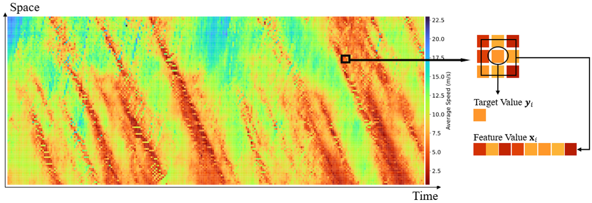
Feature and target value mapping in time–space diagram.

A significant challenge for the direct application of Equation 2 arises under high data sparsity. When a target cell’s spatiotemporal neighbors are missing, a reliable distance calculation and weighted average become impossible. This prevents the standard KNN algorithm from functioning. To address this critical limitation, this study introduces an adaptive iterative mechanism, as shown in Figure 2. The core principle of this framework is to progressively populate the TSD by prioritizing imputations based on data availability. The algorithm operates in iterations, and in each iteration N, it strategically identifies all missing cells for which a complete or sufficient eight-neighbor feature vector can be constructed from the currently available observed and previously imputed data. The modified KNN is then applied to these “high-confidence” cells, and their values are updated within the TSD. This newly imputed data is immediately incorporated into the data set, effectively expanding the pool of available information (i.e., refining the feature set) for the subsequent iteration, N + 1. This self-adaptive process repeats, leveraging newly imputed values to solve progressively more difficult gaps, until all missing values have been imputed or the process converges to a stable state. This iterative approach ensures the imputation process remains robust and effective, even when a significant proportion of the data is randomly missing, by intelligently using high-confidence estimations to unlock subsequent, more challenging imputations.

Figure 2.

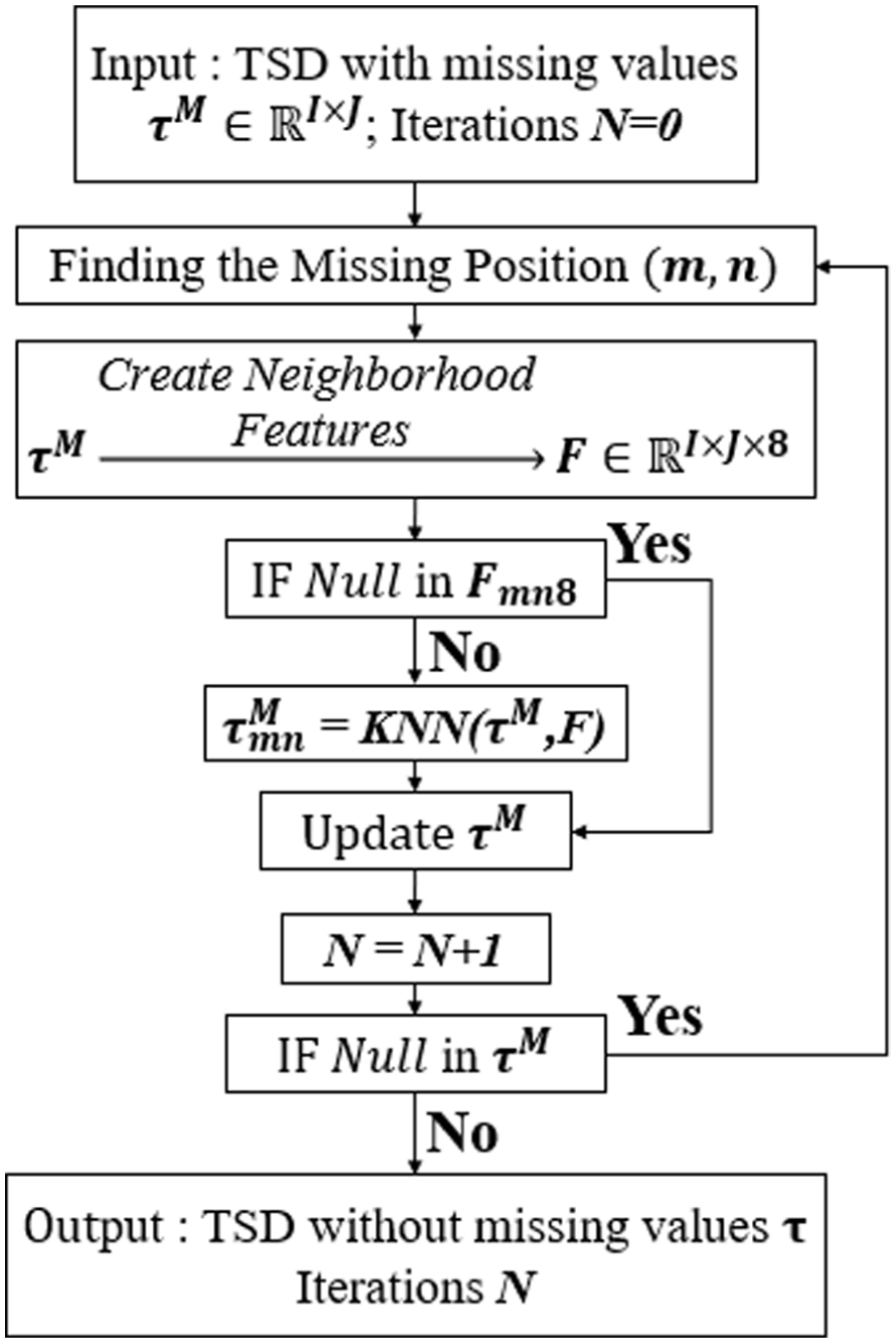
Modified K-nearest neighbor (KNN) algorithm for time–space diagram (TSD) imputation.

A notable characteristic of the KNN algorithm is that it does not involve an explicit training phase; as a nonparametric method, its training complexity is effective o(1). The computational burden is concentrated in the imputation (prediction) phase. The proposed modified KNN framework is iterative, as described in the previous section. This iterative design, which is essential for handling high sparsity, defines its practical computational cost. The total imputation complexity of this framework is approximately o(T·N_m·N_o·D), where T represents the number of iterations required for convergence, N_m represents the number of missing points, $N_{0}$ is the number of observed points, and D is the feature dimension (D = 8 in the first-order neighborhood).

Although DL can learn nonlinear feature representations, its numerous hidden layers and neurons make it significantly more complex, requiring extensive, computationally expensive offline training and managing many parameters. In sharp contrast, this modified KNN algorithm remains nonparametric, which drastically simplifies model tuning and enhances implementation stability. Therefore, this framework’s balance of zero training cost and predictable, manageable imputation complexity could efficiently meet engineering requirements, rapidly providing reliable initial solutions for sophisticated traffic management analyses.

Theoretical Foundation and Convergence Analysis

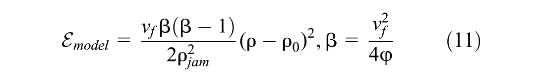
The modified KNN framework is a nonparametric, data-driven method. To provide a theoretical justification for its design, particularly the use of a weighted average of spatiotemporal neighbors, this section develops an analytical framework to explore the fundamental error propagation dynamics in TSD imputation. This framework is built on the classic Lighthill–Whitham–Richards (LWR) traffic flow model. It should be emphasized that the purpose of this analysis is to offer theoretical motivation and to demonstrate that under idealized conditions, the error of a local weighted estimation process is bounded and convergent. This provides a foundational rationale for this algorithm’s stability and effectiveness, rather than serving as a direct mathematical proof of the KNN algorithm.

Given the one-dimensional (1D) traffic flow conservation law based on the LWR traffic flow model ( 33 , 34 ).

\frac{\partial ρ}{\partial t} + \frac{\partial (ρ v)}{\partial x} = 0

(3)

where $ρ (x, t)$ represents traffic density at position x and time t, and $v (ρ) = v_{f} (1 - {(\frac{ρ}{ρ_{jam}})}^{β})$ represents the velocity–density relationship, where v_f represents free-flow speed, ρ_jam represents jam density, and β= 1 for low-density highway conditions $ρ << ρ_{jam}$ . To regularize numerical solutions, an artificial diffusion term is introduced, yielding the modified equation.

\frac{\partial ρ}{\partial t} + \frac{\partial (ρ v)}{\partial x} = φ \frac{\partial^{2} ρ}{\partial x^{2}}

(4)

where φ controls spatial diffusion intensity ( 35 ).

The Green’s function $G (x, t; x^{'}, t^{'})$ ( 36 ), representing the response to a Dirac impulse $δ (x - x^{'}) δ (t - t^{'})$ , is derived as,

\begin{matrix} G (x, t; x^{'}, t^{'}) = \frac{1}{\sqrt{4 π φ (t - t^{'})}} \\ \exp (- \frac{{(x - x^{'} - v_{f} (t - t^{'}))}^{2}}{4 φ (t - t^{'})}) \end{matrix}

(5)

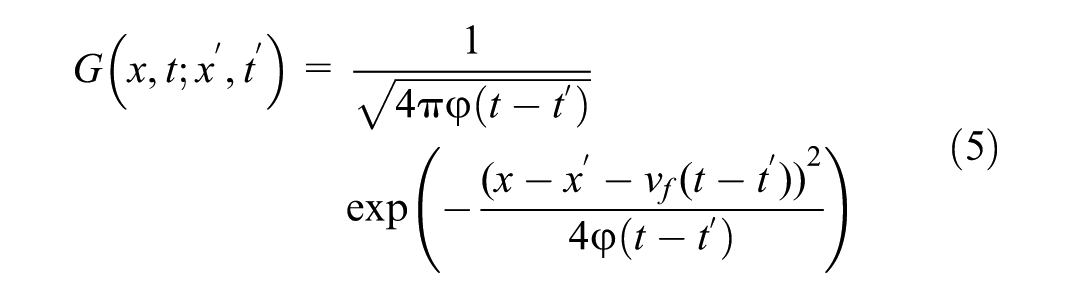
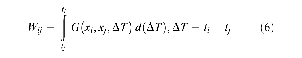
encoding convective transport v_f and diffusive smoothing φ. The weight matrix

W is constructed via temporal integration of G.

W_{ij} = \int_{t_{j}}^{t_{i}} G (x_{i}, x_{j}, Δ T) d (Δ T), Δ T = t_{i} - t_{j}

(6)

with diagonal elements quantifying historical self-influence.

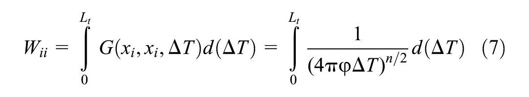
W_{ii} = \int_{0}^{L_{t}} G (x_{i}, x_{i}, Δ T) d (Δ T) = \int_{0}^{L_{t}} \frac{1}{{(4 π φ Δ T)}^{n / 2}} d (Δ T)

(7)

and off-diagonal elements.

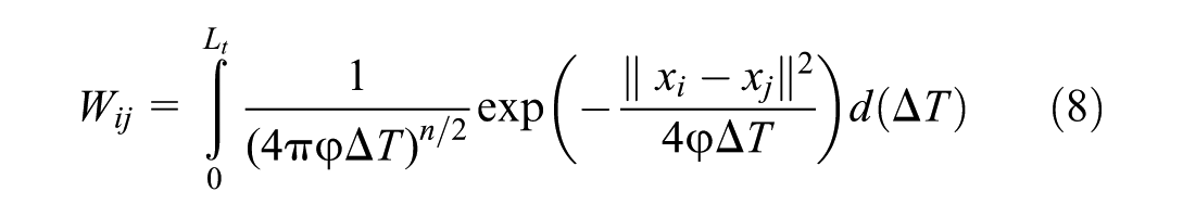
W_{ij} = \int_{0}^{L_{t}} \frac{1}{{(4 π φ Δ T)}^{n / 2}} \exp (- \frac{∥ x_{i} - x_{j} ∥^{2}}{4 φ Δ T}) d (Δ T)

(8)

For missing values $(x_{0}, t_{0})$ , the spatiotemporal neighborhood $Ω (x_{0}, t_{0}) = (x_{i}, t_{i}) | | x_{i} - x_{0} | \leq L_{x}, | t_{i} - t_{0} | \leq L_{t}$ , defines the KNN-imputed estimate.

\hat{v} (x_{0}, t_{0}) = \sum_{i = 1}^{K} w_{i} v (x_{i}, t_{i})

(9)

where w_i represents the Green’s function-derived weight . This physical model serves as the theoretical analog for the practical, data-driven weighted KNN approach. Based on this theoretical framework, the total error evolution ϵ across K iterations can be expressed as,

ϵ^{(k + 1)} (x, t) = W^{(k)} ϵ^{(k)} + b^{(k)}, b^{(k)} = E_{model}^{(k)} + E_{trunc}^{(k)}

(10)

where $E_{model}$ model represents modeling error, from the Taylor remainder of the nonlinear $v (ρ)$ .

E_{model} = \frac{v_{f} β (β - 1)}{2 ρ_{jam}^{2}} (ρ - ρ_{0})^{2}, β = \frac{v_{f}^{2}}{4 φ}

(11)

bounded by $| E_{model} | \leq C_{1} (Δ ρ_{\max})^{2}, C_{1} = \frac{v_{f} β (β - 1)}{2 ρ_{jam}^{2}}$ .

As the number of iterations increases, missing points are supplemented with weighted values, resulting in a more concentrated distribution of traffic flow density and a decrease in $Δ ρ_{\max}$ . In addition, $E_{trunc}$ represents truncation error, from Green’s function discretization.

E_{trunc} = O (Δ x^{3} + Δ t^{3})

(12)

After expanding the neighborhood samples, the truncation error can be limited to.

| ϵ_{trunc} | \leq C_{2} (\frac{Δ x}{L_{x}^{(k)}} + \frac{Δ t}{L_{t}^{(k)}})

(13)

where C₂ depends on φ and v_f; with fixed $\frac{Δ x}{L_{x}^{(k)}} = \frac{Δ t}{L_{t}^{(k)}} = 1$ .

For Equation 10, if the spectral radius of the weight matrix W is less than one, the error bound converges according to a geometric series,

∥ ϵ^{(k)} ∥ \leq ρ (W)^{k} ∥ ϵ^{(0)} ∥ + \frac{∥ b ∥}{1 - ρ (W)}

(14)

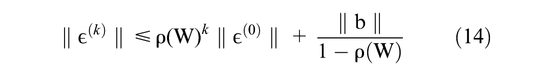
According to the Gershgorin circle theorem ( 37 ), the center of the Gershgorin disk for each row i is W_ii, with the radius $R_{i} = \sum_{j \neq i} W_{ij}$ . If $W_{ij} > R_{i}$ , then all the eigenvalues lie within the disk $| z - W_{ii} | < R_{i}$ in the complex plane, and the disk is located in the right half-plane because,

| z | \leq | z - W_{ii} | + | W_{ii} | < R_{i} + W_{ii} < 2 W_{ii}

(15)

In reality, $W_{ij} > R_{i}$ , and the spectral radius strictly satisfies,

ρ (W) \leq \max_{i} (W_{ii} + R_{i}) < 2 W_{ii}

(16)

In practical settings, compared with the scale of the TSDs, L_x and L_t are sufficiently small to ensure that $ρ (W) < 1$ .

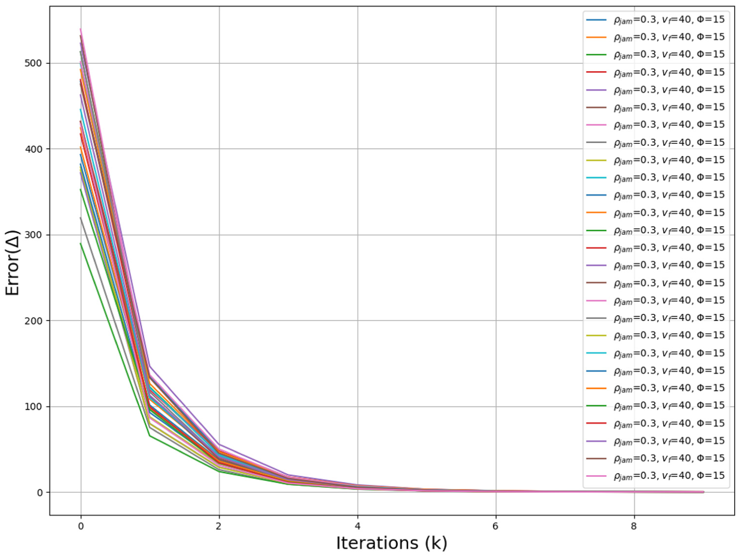
To validate this theoretical convergence, the numerical simulation results are shown in Figure 3. It is crucial to clarify that this is a theoretical simulation designed to test the convergence of the derived framework. The parameters analyzed, free-flow velocity v_f, jam density $ρ_{jam}$ , and diffusion coefficient φ, are hypothetical values chosen for this simulation to represent a range of traffic conditions. The simulation imputes data for a 2,000 m segment ( $Δ x$ = 50 m, $Δ t = 5 s$ ) using K = 3. As Figure 3 shows, the cumulative error $Error (Δ)$ rapidly converges within the initial few iterations across all tested parameter settings and missing data rates. This simulation confirms the theoretical stability of the local weighted averaging approach, satisfying the requirements for practical engineering applications. The sensitivity analysis for other missing cases can be found in Appendix A.

Figure 3.

Sensitivity analysis results under 10% missing rate.

Note that Error(Δ) denotes the cumulative error between the imputed results and the original data on the TSD.

Experiments and Discussions

Data Set Description

To ensure a fair evaluation of the modified KNN algorithm’s effectiveness in TSD imputation, three representative trajectory data sets were selected from diverse traffic environments, which have different traffic flow and road conditions.

Next Generation Simulation (NGSIM) ( 38 ): Highway section US-101 in Los Angeles, US, capturing complex weaving traffic flows.

HighD ( 39 ): German highway naturalistic trajectories from RWTH Aachen University, reflecting free-flow conditions.

Ubiquitous Traffic Eyes (UTE) ( 40 ): RML-7 highway section in Nanjing, China, representing mixed traffic operations.

Detailed information on the three data sets is provided in Table 1.

Table 1.

Description of Detailed Information in Three Data Sets

Indicators	NGSIM	HighD	UTE
Sampling frequency (s)	0.1	0.025	0.03
Effective data volume (vehicle)	2,097,023	770,895	203,161
Temporal length (s)	2,235	1,103	158
Spatial length (m)	672	369	237
Number of lanes	5	6	4

Note: NGSIM = Next Generation Simulation; UTE = Ubiquitous Traffic Eyes.

The trajectory data from aerial video sources introduces inherent perspective distortions, causing spatiotemporal positioning errors in road boundary and entry/exit zone detection ( 41 ). The TSD reliability is enhanced by systematically excluding terminal zones during preprocessing. The experimental framework establishes two spatiotemporal resolutions.

Fine-grained TSD (10 m × 1 s): Minimum spatial resolution of 10 m (encompassing ≥ 2 typical vehicles) with 1-s temporal granularity, achieving sub-vehicle-level traffic state characterization.

Benchmark TSD (20 m × 5 s): Coarser-resolution baseline for comparative analysis.

To simulate the various levels of data corruption found in real-world scenarios, missing values were introduced into the processed TSDs. This study focuses on the missing completely at random pattern, which was implemented by randomly selecting and removing a specific percentage of individual cells from the TSD matrix, independent of their spatiotemporal location or underlying speed value. The severity of data corruption was adjusted by controlling this random missing ratio across five levels: 10%, 20%, 30%, 40%, and 50% ( 42 ).

Baseline Models and Experimental Indicators

To comprehensively evaluate the performance of the proposed modified KNN algorithm, its effectiveness is benchmarked against a diverse set of established and advanced methods for TSD imputation. Recognizing the need to position this computationally efficient approach within the broader landscape of imputation techniques, baselines were included from classic statistical models to contemporary DL architectures. Advanced DL methods often achieve high accuracy by modeling complex nonlinear dependencies; their significant computational demands, large parameter counts, and requirements for extensive training data can limit practical deployment in a real time ITS. Therefore, this comparison includes computationally intensive and lightweight models to provide a holistic assessment of the accuracy–efficiency trade-off. The selected baseline models for comparison in this study are as follows.

Multivariate Linear Regression

Inspired by the approach proposed in the literature ( 4 ), this model utilizes the spatiotemporal features derived from the eight adjacent cells (first-order spatial neighborhood) to predict the value of a target cell. The MLR model was implemented noniteratively: it was trained once on all available data points in the sparse TSD to fit a single linear model, which was then used to predict all missing values simultaneously.

Alternating Least Squares With SoftImpute

This method is an efficient algorithm for matrix completion using nuclear norm regularization. It approximates the underlying low-rank structure of the TSD matrix via fast alternating least squares. The implementation utilizes a rank approximation and iterates until convergence or a maximum of iterations. The corresponding software package, SoftImpute, is designed for matrix imputation ( 43 ).

Kalman Filter

A KF is a classic, widely used method for time series state estimation and smoothing. For TSD imputation, it was adapted by treating each spatial row of the TSD as an independent 1D time series. A 1D Kalman smoother is applied row-wise, assuming a simple constant velocity model. The KF smoother efficiently imputes missing values based on temporal correlations within each spatial slice, with a computational cost primarily dependent on the TSD dimensions rather than the missing rate ( 44 ).

Traffic State Reconstruction Generative Adversarial Network

This model employs a GAN architecture specifically designed to reconstruct spatiotemporal traffic states. This implementation follows a typical GAN training strategy involving a generator and a discriminator. The training includes a pretraining phase using pixel-wise and scale distribution losses, followed by adversarial fine-tuning for each specific missing rate using a relativistic least squares GAN loss combined with the pretraining losses ( 7 ).

The mean absolute percentage error (MAPE) is employed as the evaluation metric. The formula for MAPE is as follows:

MAPE = \frac{1}{n} \sum_{i = 1}^{n} | \frac{y_{i} - {\hat{y}}_{i}}{y_{i}} | \times 100 %

(17)

where y_i represents the actual speed values in the ith cell of TSD and ${\hat{y}}_{i}$ represents the speed values imputed by the modified KNN algorithm. Of note, the parameters of the MLR models calculated from the different data sets for different conditions are shown in Appendix B.

In addition, the total computational time required by each model to complete the TSD imputation task is recorded as a key indicator of computational efficiency and practical deployability. This metric is defined as the sum of two components: (1) training time; and (2) imputation time, providing a comprehensive measure of the overall computational overhead associated with using each method for a given imputation task (the specific CPU configuration for completing the experiment is Intel (R) Core (TM) i9-10940X CPU @ 3.30 GHz (28 CPUs), ∼ 3.3 GHz).

Parameters of the Modified KNN Model

A key advantage of the proposed modified KNN algorithm is its parsimony, relying primarily on a single parameter: the number of nearest neighbors K. This section details the investigation into the model’s sensitivity to K and presents a practical empirical formula for estimating an optimal value, enhancing the model’s usability in real-world applications.

To understand the effect of K on imputation performance, the optimal value was determined by systematically traversing K values of 2–10 across all 30 experimental conditions. The relationship between K and the resulting MAPE is shown in Figure 4. The results reveal a consistent trend in most scenarios (e.g., Figure 4, a, b, d, e, f): the error typically exhibits a U-shaped relationship with K. Initially, as K increases from a small value, the error decreases. This is probably because incorporating more neighbors helps to average out noise and capture the underlying traffic state more reliably. However, beyond a certain optimal point (often found between K = 3 and K = 8 in these tests, see Appendix C for optimal values), further increasing K leads to a rise in error. Selecting too many neighbors, especially those spatiotemporally distant, can introduce irrelevant information or patterns from dissimilar traffic conditions, increasing the risk of mismatch and degrading imputation accuracy, which reflects the classic bias-variance trade-off inherent in KNN models. A notable exception is observed in the high-resolution NGSIM data set (Figure 4c), where the error consistently decreases as K increases within the tested range [2, 10]. This does not necessarily contradict the general U-shaped trend but suggests that for large-scale, complex data sets with potentially richer patterns, the optimal K might lie beyond the traversed range. The flattening of the error curve at larger K values in Figure 4c supports this speculation. While exploring K > 10 could be beneficial for such specific cases, the range [2, 10] provided effective results across the majority of conditions in this study. This analysis underscores that the optimal choice of K is influenced by factors such as data set size, traffic complexity, and data sparsity.

Figure 4.

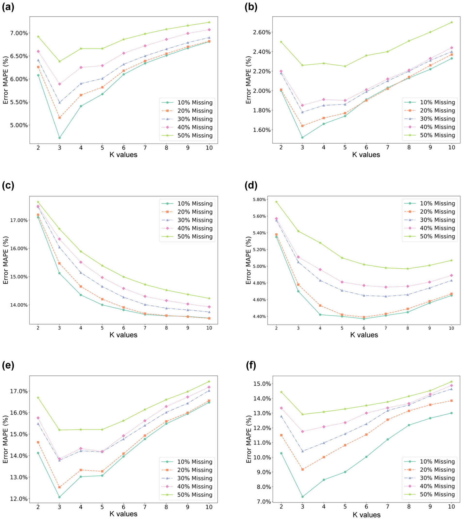
Modified K-nearest neighbor (KNN) model errors for different values of K in different cases: (a) HighD 1 s × 10 m; (b) HighD 5 s × 20 m; (c) NGSIM 1 s × 10 m; (d) NGSIM 5 s × 20 m; (e) UTE 1 s × 10 m; and (f) UTE 5 s × 20 m.

Given the observed relationship between K, MAPE, missing rate (MR), and data set size N, defined as the number of available spatiotemporal data points in the TSD, and motivated by the need for a practical method to select K without extensive traversal, an empirical formula is proposed. Based on the analysis shown in Figure 4, the imputation error is modeled using a quadratic polynomial that incorporates K, MR, and N, including linear, quadratic, and interaction terms.

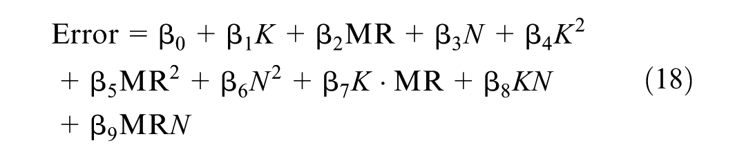
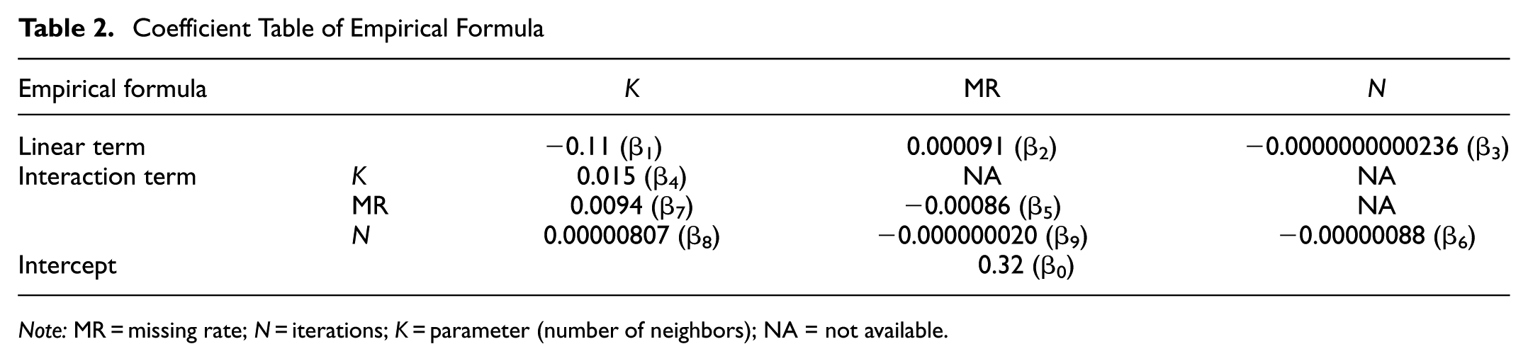
\begin{matrix} Error = β_{0} + β_{1} K + β_{2} MR + β_{3} N + β_{4} K^{2} \\ + β_{5} {MR}^{2} + β_{6} N^{2} + β_{7} K \cdot MR + β_{8} K N \\ + β_{9} MR N \end{matrix}

(18)

An ordinary least squares regression is employed to derive the coefficients. The regression was fitted using data points (K, MR, N, and Error) pooled from all 30 experimental conditions across the three data sets. Before fitting, MAPE values across all conditions were normalized to ensure comparability and allow for integrated analysis. The resulting coefficients are presented in Table 2. The goodness-of-fit for this empirical formula is shown in Figure 5, where the high coefficient of determination R² values (from 0.78 to 0.97) across the diverse data sets and resolutions confirm that the quadratic model effectively captures the underlying relationship between K and imputation error, substantiating the modeling hypothesis.

Table 2.

Coefficient Table of Empirical Formula

Empirical formula		K	MR	N
Linear term		−0.11 (β₁)	0.000091 (β₂)	−0.0000000000236 (β₃)
Interaction term	K	0.015 (β₄)	NA	NA
	MR	0.0094 (β₇)	−0.00086 (β₅)	NA
	N	0.00000807 (β₈)	−0.000000020 (β₉)	−0.00000088 (β₆)
Intercept		0.32 (β₀)

Note: MR = missing rate; N = iterations; K = parameter (number of neighbors); NA = not available.

Figure 5.

Fitting effect of correlation between K values and errors: (a) HighD 1 s × 10 m; (b) HighD 5 s × 20 m; (c) NGSIM 1 s × 10 m; (d) NGSIM 5 s × 20 m; (e) UTE 1 s × 10 m; and (f) UTE 5 s × 20 m.

The coefficients presented in Table 2 provide insights into how each factor influences the imputation error. The intercept (β₀ = 0.32) serves as a baseline normalized error under theoretical zero conditions. Linear terms, such as the negative coefficient for K (β₁ = –0.11), reflects the initial error reduction observed as K increases from small values (consistent with Figure 4). Quadratic terms, such as the positive coefficient for K² (β₄ = 0.015), capture the characteristic U-shaped curve, ensuring the error eventually increases as K becomes excessively large. Furthermore, interaction terms model the interplay between factors; for example, the positive $K MR$ coefficient (β₇ = 0.0094) suggests that the effect of increasing K might vary depending on the level of data sparsity.

Because this empirical formula was derived from pooled data encompassing diverse traffic conditions and experimental settings (sparsity, resolution), it is expected to possess reasonable transferability for estimating a near-optimal K value in similar highway TSD imputation tasks. Data set-specific fine-tuning might yield marginal improvements; this formula offers a valuable and computationally inexpensive starting point. In practice, when encountering a new TSD, the MR and N can be determined, and the formula can be applied. The optimal integer value for K can be estimated by finding the value of K where the partial derivative of Equation 18 for K is zero, for instance, by solving $\frac{\partial Error}{\partial K} = β_{1} + 2 β_{4} K + β_{7 MR} + β_{8} N = 0$ for K, and rounding to the nearest integer, which avoids the substantial computational cost associated with iterative K value searching, significantly enhancing the model’s efficiency and deployment potential in practical ITS applications, particularly those requiring rapid responses.

Effect Analysis of Imputation

Using the imputation process of the NGSIM data set with a cell size of 1 s× 10 m and an MR of 50% as an example to show the modified KNN’s mechanism. With the optimal K value obtained through traversal, the model required only three iterations to fill in all the missing values. The imputation process is shown in Figure 6.

Figure 6.

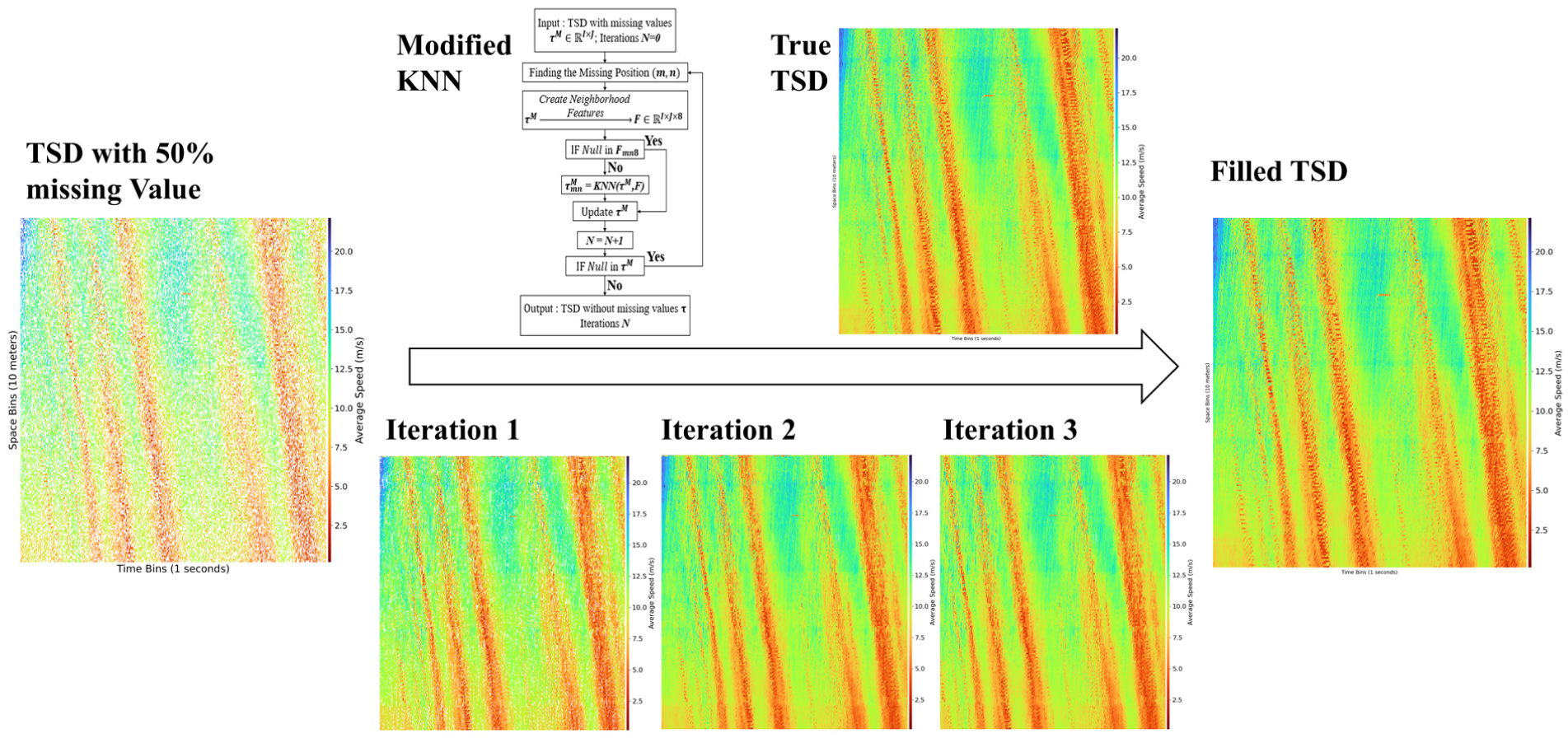
Example of imputation process.

Comparative results for imputation accuracy, shown in Figure 7, reveal nuanced performance characteristics across the models. The DL approach, TSR-GAN, frequently achieved the lowest MAPE, particularly at lower resolutions and intermediate MRs at high resolution; its advantage was not universal, especially considering its computational overhead. The proposed modified KNN demonstrated remarkably strong and consistent performance, often yielding MAPE values very close to, and in several instances exceeding, those of TSR-GAN. The modified KNN consistently outperformed MLR, SoftImpute, and KF across nearly all scenarios, showcasing superior accuracy and robustness, especially as data sparsity increased. For example, on the challenging NGSIM 1 s × 10 m data set with 50% missing data, the modified KNN’s MAPE was substantially better than MLR, SoftImpute, and KF. The SoftImpute model showed notable strength on the UTE 1 s × 10 m data set, achieving the best accuracy among non-DL methods at higher missing rates (e.g., 12.04% MAPE at 50% missingness), aligning with observations about potential data set-specific suitability. However, its performance on NGSIM was less competitive. The MLR generally exhibited higher errors than the modified KNN, particularly at high missing rates, reinforcing concerns about its stability. The KF, while computationally stable, typically yielded moderate accuracy, often falling behind the modified KNN and TSR-GAN.

Figure 7.

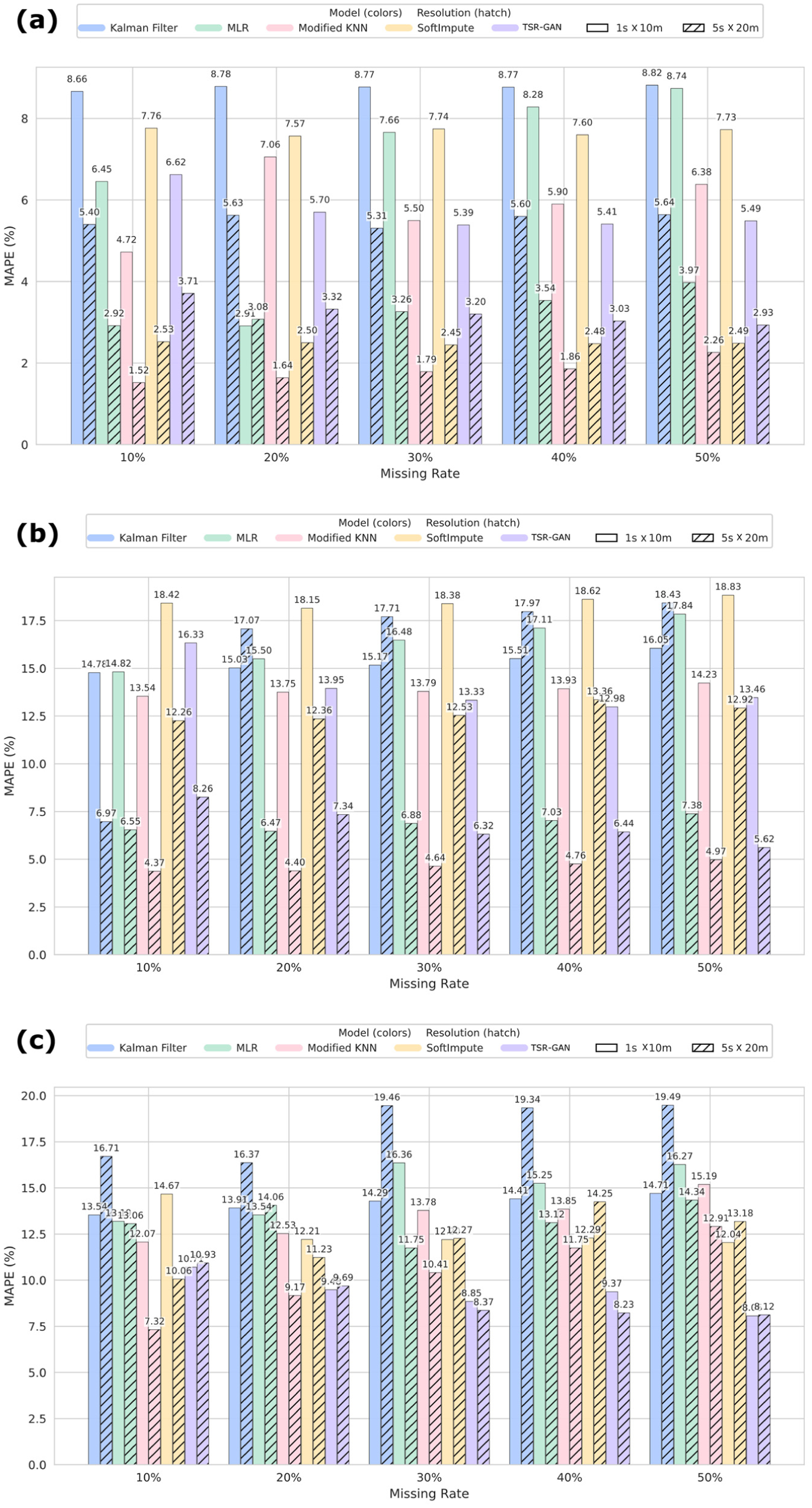
Comparison of model’s MAPE under different conditions: (a) HighD, (b) NGSIM, and (c) UTE.

The analysis of computational efficiency, shown in Figure 8, highlights stark differences in resource requirements. The TSR-GAN consistently demanded the highest computational time, often requiring 10 s or even over 100 s per run, reflecting the intensive nature of the DL model training and inference. In contrast, MLR and SoftImpute consistently demonstrate low computational overheads. The computational time for the modified KNN and KF is data set-dependent but remains significantly lower than that of TSR-GAN. Their execution times showed only marginal increases with rising missing rates, positioning them as computationally lightweight options. The KF occupied an intermediate position; its execution time was significantly higher than the MLR, modified KNN, and SoftImpute, but substantially lower than TSR-GAN, and notably stable across different missing rates because of its noniterative, row-wise processing structure.

Figure 8.

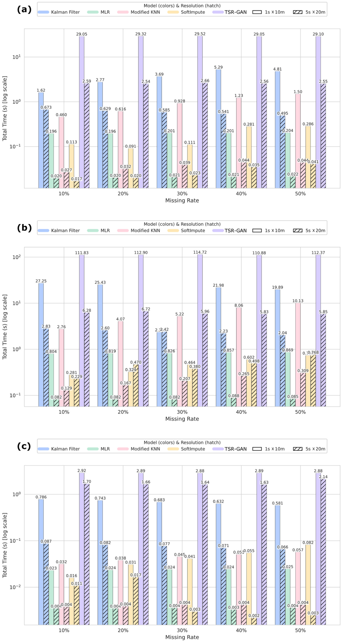
Comparison of model’s computational efficiency under different conditions: (a) HighD; (b) NGSIM; and (c) UTE.

Synthesizing these findings, Figure 9 shows a distinct accuracy–efficiency landscape. TSR-GAN occupies the high accuracy, high-cost corner. In addition, MLR and SoftImpute are low-cost options but often compromise on accuracy or consistency. The KF offers stable, moderate performance and efficiency. The proposed modified KNN algorithm distinguishes itself by occupying a highly advantageous position in this landscape. It delivers accuracy that is consistently among the best, frequently rivaling or exceeding the state-of-the-art DL model, especially at lower resolutions, while maintaining exceptional computational efficiency comparable with the simplest baseline methods. This compelling combination of high accuracy, robustness against data sparsity, and minimal computational overhead makes the modified KNN algorithm a highly practical and effective solution for TSD imputation. Its consistent performance across diverse international data sets further supports its strong transferability and generalizability, rendering it suitable for objective benchmarking and deployment in various ITS contexts where balancing accuracy and efficiency is paramount.

Figure 9.

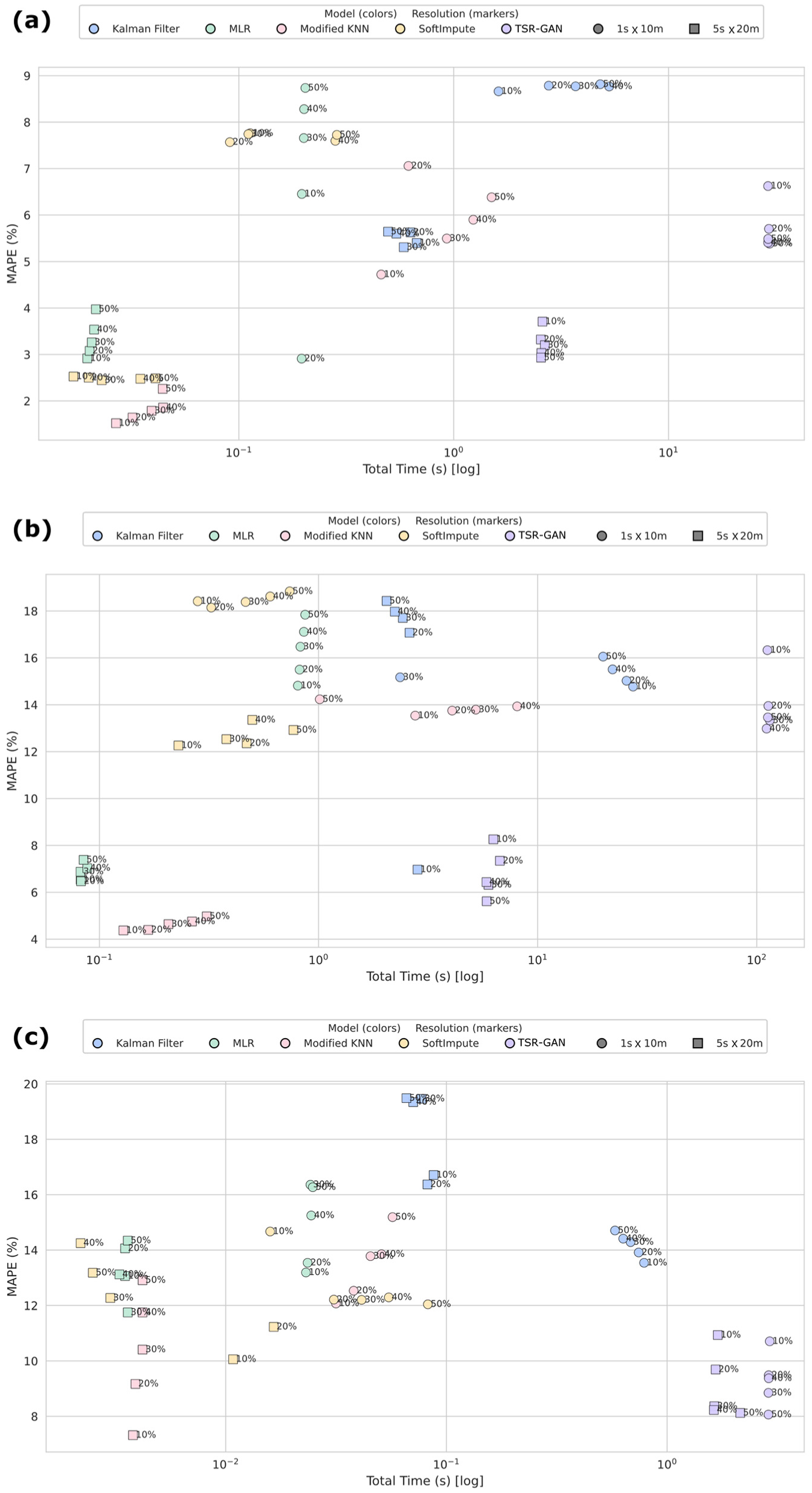
Accuracy–efficiency trade-off of time–space diagram (TSD) imputation models under different conditions: (a) HighD; (b) NGSIM; and (c) UTE.

Influence of Neighborhood Order on Imputation Performance

Selecting appropriate features is crucial to the performance of KNN algorithms. In spatiotemporal data such as TSDs, the neighborhood used to extract features defines the model’s receptive field and influences its ability to capture relevant local traffic dynamics. To systematically investigate the effect of this receptive field size on imputation accuracy, a comprehensive set of experiments was conducted. The “Neighborhood Order” is defined based on the spatial and temporal adjacency layers around a target cell within the TSD grid. Order 1 corresponds precisely to the first-order spatial neighborhood used throughout this study, encompassing the immediate eight neighboring cells surrounding the target cell. Order 2 expands this to include the 24 cells forming the next layer outward (a 5 × 5 grid excluding the central 3 × 3 grid). Similarly, Order 3 includes the subsequent layer of 48 cells (a 7 × 7 grid excluding the central 5 × 5 grid). For each order, the observed values (speeds) within the corresponding neighborhood cells were used as the feature vector for the KNN model. Imputation performance was evaluated across three neighborhood orders across all experimental conditions: three distinct data sets, two spatiotemporal resolutions, and five random missing data rates. The optimal K value determined previously for the first-order neighborhood was used for all orders within each condition for consistency.

The experimental results, shown in Figure 10, reveal a clear and consistent trend across all tested scenarios. The KNN model utilizing the first-order neighborhood consistently achieves the lowest MAPE, indicating the highest imputation accuracy. As the neighborhood order increases from first to second, and then to third, the model’s performance exhibits a persistent and significant degradation, manifested as a marked increase in imputation error. This seemingly counterintuitive outcome, where incorporating more spatiotemporal information leads to poorer results, highlights a fundamental aspect of applying instance-based learning methods such as KNN to traffic flow data. The first-order neighborhood appears to capture the most relevant and highly correlated contextual information necessary for accurately estimating the state of the target cell; this immediate vicinity constitutes the core predictive signal. In contrast, expanding the receptive field to second and third orders introduces information from a broader spatial-temporal region; the correlation between these more distant neighbors and the target cell diminishes rapidly. These distant cells are more likely influenced by different traffic dynamics or perturbations (e.g., upstream bottlenecks or downstream spillbacks occurring further away in time or space), which predominantly act as irrelevant noise or confounding factors within the feature vector. An abundance of such low-correlation features impairs the algorithm’s ability to identify genuinely similar spatiotemporal patterns based on the distance metric, leading to suboptimal neighbor selection and less accurate imputation. In addition, the consistency of this finding across three data sets reflecting diverse traffic characteristics and driving behaviors strongly suggests that for the task of local TSD imputation, the most critical predictive information is invariably contained in the immediate spatiotemporal vicinity. This reinforces the suitability of the first-order spatial neighborhood as the feature extraction method for the proposed modified KNN algorithm and underscores the importance of leveraging local correlations in TSD data imputation.

Figure 10.

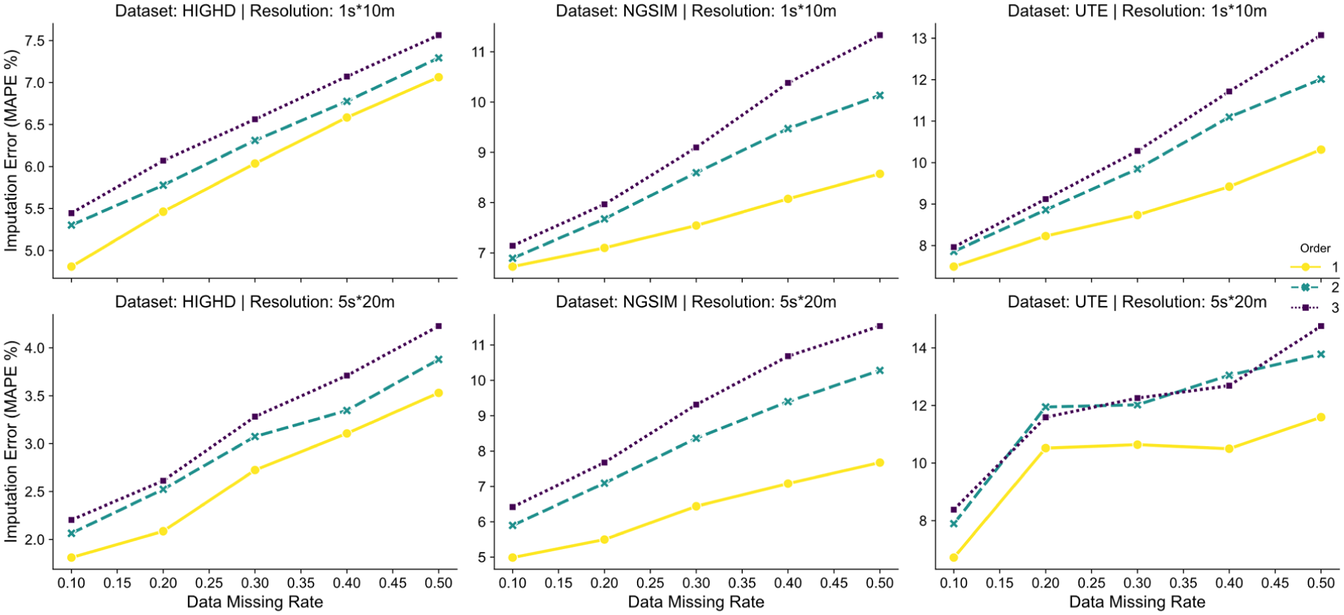
Influence of neighborhood order on imputation performance.

Analysis of Imputation Error Distribution Across Traffic Regimes

To investigate potential biases and assess the robustness of the modified KNN model under varying traffic states, a detailed analysis of the conditional distribution of imputation errors across distinct speed regimes was conducted. For each data set, the free-flow speed was estimated as the 90th percentile of all observed speeds pertaining to that segment. This 90th percentile threshold is utilized as a robust estimator, effectively approximating the unconstrained vehicular speed while remaining insensitive to anomalous low-speed observations. Subsequently, each 5-min interval was classified based on the ratio of its interval mean speed to the estimated free-flow speed. An interval was classified as “Congested-Flow” if the ratio was below 0.6 ( 45 ). The MAPE for each imputation was classified into four bins: 0%–5%, 5%–10%, 10%–20%, and > 20%. Then, the conditional probability distributions were computed, representing the proportion of errors in each speed regime falling into each error category. To statistically assess whether the observed differences in these conditional distributions were significant, indicating a dependence between error magnitude and speed regime, Pearson’s chi-squared $χ^{2}$ . test of independence was applied to the underlying 2 × 4 observed frequency tables for each of the 30 experimental conditions.

χ^{2} = \sum \frac{{(O_{i} - E_{i})}^{2}}{E_{i}}

(19)

where O_i represents the observed frequency in cell i of the contingency table and E_i represents the expected frequency in cell i under the null hypothesis of independence between speed regime and error bin. The resulting p-values were compared against a significance level of α = 0.05.

The test results shown in Figure 11 revealed statistically significant evidence (p < 0.05) of dependence between the error distribution and speed regime in the vast majority of tested conditions, particularly as the MR increased beyond 10% or 20% across all data sets and resolutions. The consistently significant p-values, often below 0.001, strongly suggest the presence of a systematic bias effect in the modified KNN model’s performance relative to the prevailing traffic state. Although warnings for low expected frequencies occasionally arose, primarily at the 10% MR or in the high accuracy HighD (20 m × 5 s) case, the persistent significance across numerous conditions lends confidence to the overall finding of dependence. In addition, the congested-flow regime consistently exhibits a markedly higher proportion of large errors (> 20%) compared with the free-flow regime. This disparity generally widens as the missing data rate increases. In contrast, the free-flow regime consistently demonstrates a significantly higher proportion of very small errors (0%–5%) compared with the congested-flow regime in almost all conditions where bias was statistically detected.

Figure 11.

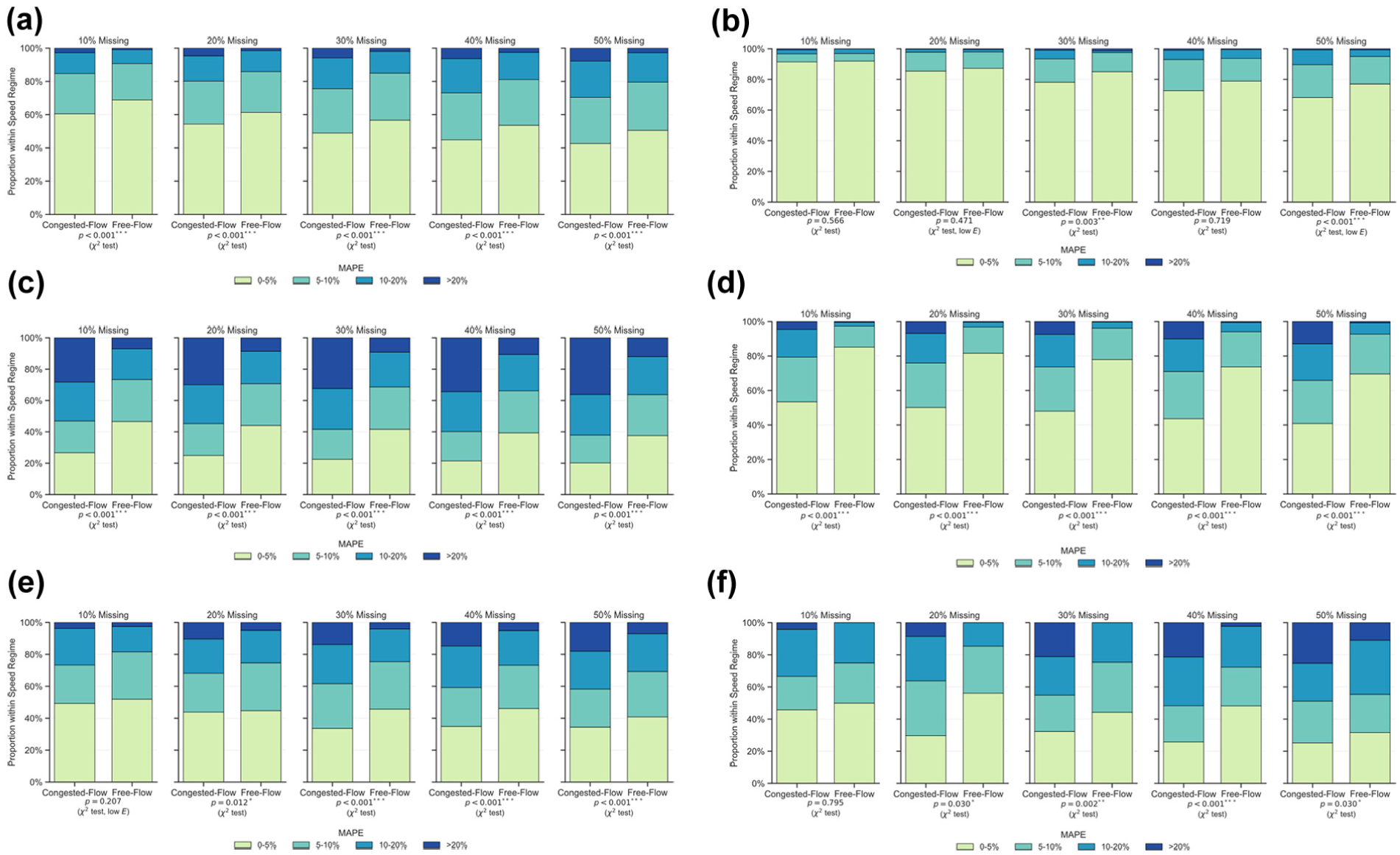
Conditional distribution of modified KNN imputation errors by speed regime and MR: (a) HighD (10 m × 1 s); (b) HighD (20 m × 5 s); (c) NGSIM (10 m × 1 s); (d) NGSIM (20 m × 5 s); (e) UTE (10 m × 1 s); and (f) UTE (20 m × 5 s).

These findings suggest that the modified KNN model’s reliability is contingent on the traffic state being imputed. It appears less robust when estimating speeds during congested conditions compared with free-flow conditions. The inherent increase in speed variability and potentially more complex spatiotemporal dynamics characteristic of congestion probably challenge the KNN algorithm’s core assumption of local similarity, making it harder to find truly representative neighbors and increasing the likelihood of large percentage errors. The model demonstrates strong performance in smoother, high-speed traffic, characterized by a higher concentration of low-magnitude errors; its tendency toward larger deviations in congested regimes represents a notable bias.

Cross-Filling Across Data Sets

The fundamental dynamic characteristics of traffic flow, influenced by human behavior and infrastructure design, exhibit a certain degree of universality. For instance, congestion patterns during peak hours tend to follow similar rules across different areas ( 46 ). When dealing with data sets with high MRs, transferring knowledge from other data sets for imputation is currently an effective solution ( 18 , 47 ). The modified KNN model for imputing missing values in TSDs relies on finding similar spatiotemporal neighborhood features. This simple framework allows the model’s knowledge transfer capabilities to be explored across different data sets. To investigate cross-filling across data sets, a straightforward cross-dataset imputation scheme is designed. It is inferred that dimensional consistency is necessary for a simple model, such as a KNN, to effectively match different data sets. After normalization, differences in dimensions and ranges of data sets are eliminated, enhancing the comparability of traffic characteristics between different data sets. Therefore, the speed data from the three data sets need to be normalized. The normalization results are shown in Figure 12.

Figure 12.

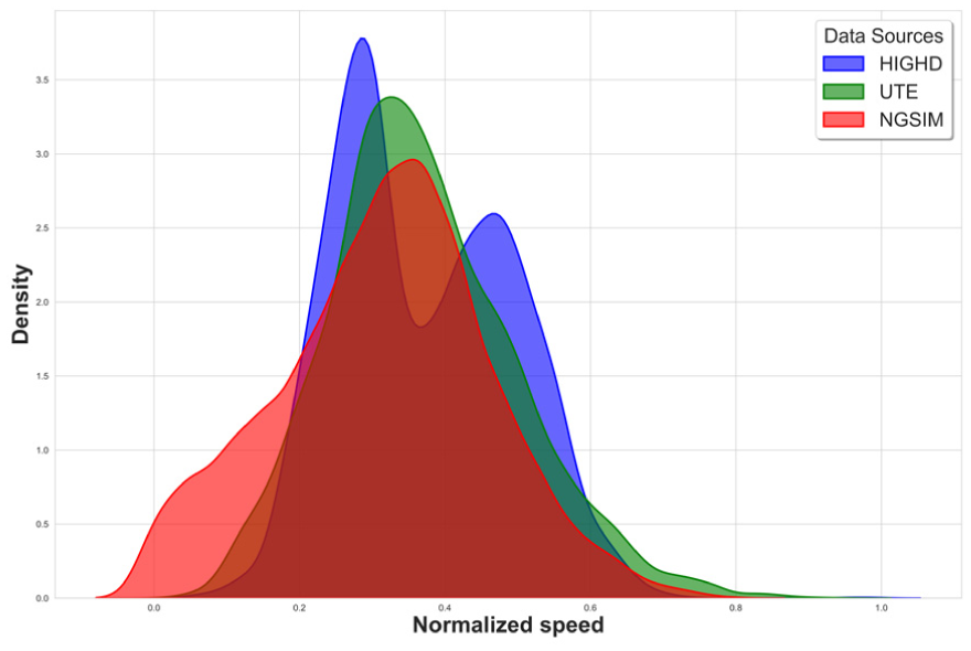
Normalized distribution of three data sets.

Define the sample library for different data sets as Y^j, with the corresponding spatiotemporal neighborhood features as X^j. For a specific sample $y_{0}^{j}$ , the formula for cross-data set imputation using KNN is as follows:

{\hat{y}}_{0}^{j} = \frac{\sum_{i = 1}^{k} α_{i} y_{i}^{m}}{k}, m \neq j

(20)

where $x_{i}^{m}$ represents a sample in data set m that is similar to $x_{0}^{j}$ in data set j, $y_{i}^{m}$ represents the observed value corresponding to $x_{i}^{m}$ , and α_i represents the correction factor.

To simplify the experiment, the spatiotemporal cell scale was fixed at 5 s×20 m, the number of neighbors was five, and the MR at 10%, using MAPE as the error metric. Jensen–Shannon divergence (JS divergence) was used to measure the similarity between the distributions of the two data sets.

M = \frac{1}{2} (P + Q)

(21)

D_{JS} (P ∥ Q) = \frac{1}{2} \sum_{i} P (i) \log \frac{P (i)}{M (i)} + \frac{1}{2} \sum_{i} Q (i) \log \frac{Q (i)}{M (i)}

(22)

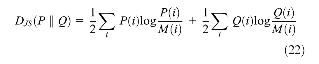
where P and Q represent two different distributions, where lower JS values indicate higher distribution similarity. Table 3 highlights that the accuracy of the cross-data set imputation scheme based on the modified KNN model is basically maintained at a high level. Paired data sets with lower JS divergence values exhibit better imputation performance, indicating that distribution similarity significantly affects the imputation outcome. In cases with higher JS divergence values, multisource imputation performs significantly better than single-source imputation. For example, using both HighD and UTE data sources to impute the UTE data set yields better results than using a single data source. In addition, the imputation effectiveness depends on distribution similarity and the quality and richness of the data sets. Although cross-imputation did not achieve the same level of accuracy as self-imputation within the same data set, it still maintained a high degree of accuracy. This result may be attributed to the high acquisition accuracy and quality of the selected datasets. Therefore, for lower-quality data sets or those lacking sufficient spatiotemporal neighborhood features, self-imputation methods are impractical. In these cases, the value of cross-data set imputation methods becomes more apparent. Designing a reasonable transfer learning framework based on modified KNN methods for cross-data set traffic flow imputation is a direction for future work.

Table 3.

Cross-Data Set Imputation Results

Filled data sets	Data sets for filling	JS divergence value	Single data source effect (%)	Multiple data source effect (%)
HighD	NGSIM	0.1277	10.27	10.30
HighD	HighD	UTE	0.1994	14.19
NGSIM	HighD	0.1277	12.15	10.66
NGSIM	NGSIM	UTE	0.1708	10.56
UTE	HighD	0.1994	35.41	20.04
UTE	UTE	NGSIM	0.1708	19.12

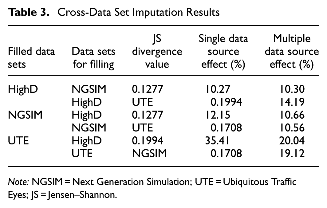
Note: NGSIM = Next Generation Simulation; UTE = Ubiquitous Traffic Eyes; JS = Jensen–Shannon.

Conclusion

The traffic TSD remains a fundamental and efficient tool for visualizing traffic flow dynamics in transportation research and practice. However, data sparsity, stemming from limitations in sensing infrastructure, often hinders the construction and utility of high-resolution TSDs, obscuring crucial details of traffic dynamics. While advanced DL frameworks have demonstrated high precision in imputation tasks, their substantial computational demands, significant parameter counts, and reliance on extensive training data often limit their practical applicability, particularly in resource-constrained or real time ITS environments.

To address these limitations by balancing accuracy and efficiency, this study proposed and evaluated a modified KNN framework incorporating spatiotemporal weighting and an adaptive iterative process for imputing missing data in high-resolution TSDs. Furthermore, theoretical motivation on the stability and convergence of these local weighted averaging methods was provided using analysis inspired by Green’s function within an idealized traffic flow model context, supported by numerical simulations. The adaptive iterative mechanism proved crucial for handling high missing rates effectively, enabling robust imputation while maintaining the model’s inherent simplicity, relying primarily on a single key parameter, K. Rigorous validation was performed using diverse trajectory datasets from the United States (NGSIM), Germany (HighD), and China (UTE) under 30 distinct experimental conditions encompassing two spatiotemporal resolutions and five levels of random data sparsity ranging from 10% to 50%. Compared against a comprehensive suite of baseline models, including MLR, SoftImpute with Alternating Least Squares (SoftImpute-ALS), KF, and TSR-GAN, the proposed modified KNN framework demonstrated a compelling balance between high imputation accuracy and exceptional computational efficiency. It consistently achieved accuracy competitive with, and occasionally surpassing, the computationally intensive TSR-GAN, while significantly outperforming the other baseline methods, particularly showcasing strong robustness under high data sparsity conditions. A practical empirical formula relating the optimal parameter K to data sparsity and data set size was derived via polynomial fitting on pooled data, offering an efficient method for parameter estimation in practice and significantly reducing the need for computationally expensive parameter searches. Further analysis confirmed the effectiveness of using the immediate first-order neighborhood for feature extraction, demonstrating that incorporating higher-order neighbors tended to degrade performance by introducing noise. In addition, a preliminary investigation into cross-data set imputation highlighted the model’s potential for knowledge transfer, particularly when leveraging multiple source data sets or data sets with similar underlying traffic flow distributions.

Given the importance and widespread use of TSDs, the proposed modified KNN imputation framework offers a significant contribution by providing a practical, robust, and computationally efficient tool to enhance the resolution and completeness of traffic state data. However, certain limitations should be acknowledged. The reliance on immediate spatiotemporal neighbors and Euclidean distance in feature space, while effective and computationally simple, may not fully capture all complex real-world traffic correlations. Furthermore, the analysis of error distribution revealed a tendency for the KNN model to exhibit larger percentage errors under congested conditions compared with free-flow states, indicating a potential performance bias relative to the traffic regime. Future research should be directed toward addressing these limitations. Enhancements to imputation accuracy could be pursued by exploring more sophisticated feature engineering or non-Euclidean distance metrics to better encapsulate traffic dynamics and mitigate the observed performance bias under congestion. To address scalability for large-scale TSDs, optimizations, such as KD-Tree indexing for accelerated neighbor retrieval or parallelization of the iterative process, require systematic investigation. The cross-data set imputation framework could also be enhanced by incorporating formal transfer learning techniques to improve performance in cases of extreme data sparsity. Finally, evaluating the proposed method’s performance specifically against structured missing data patterns remains an important avenue for future work.

Supplemental Material

sj-docx-1-trr-10.1177_03611981261419011 – Supplemental material for A Simple Yet Efficient K-Nearest Neighbor-Based Method for High-Resolution Traffic Time–Space Diagram Imputation

Supplemental material, sj-docx-1-trr-10.1177_03611981261419011 for A Simple Yet Efficient K-Nearest Neighbor-Based Method for High-Resolution Traffic Time–Space Diagram Imputation by Junjie Hu, Jaeyoung Jay Lee, Jun Bai and Suyi Mao in Transportation Research Record

Footnotes

Author Contributions

The authors confirm contribution to the paper as follows: study conception and design: Junjie Hu, Jun Bai; data collection: Junjie Hu; analysis and interpretation of results: Junjie Hu, Jaeyoung Jay Lee; draft manuscript preparation: Junjie Hu, Jaeyoung Jay Lee, Jun Bai, Suyi Mao. All authors reviewed the results and approved the final version of the manuscript.

Declaration of Conflicting Interests

The authors declared the following potential conflicts of interest with respect to the research, authorship, and/or publication of this article: Jaeyoung Jay Lee is on the Transportation Research Record’s Editorial Board. His role is a handling editor. This potential conflict of interest has been acknowledged by all authors, and no part of the editorial decision-making process was influenced by his involvement.

Funding

The authors disclosed receipt of the following financial support for the research, authorship, and/or publication of this article: This research was funded by the Natural Science Foundation of China under Grant No. 72471249, the Natural Science Foundation of Changsha under Grant No. kq2402221, and the Changsha Major Science and Technology Project (No. kh2401002).

ORCID iDs

Junjie Hu

Jaeyoung Jay Lee

Jun Bai

Suyi Mao

Supplemental Material

Supplemental material for this article is available online.

References

Grumert

E. F.

Tapani

Characteristics of Variable Speed Limit Systems. European Transport Research Review, Vol. 10, No. 2, 2018. https://doi.org/10.1186/s12544-018-0294-8.

Dai

Wang

Learning Traffic as Images: A Deep Convolutional Neural Network for Large-Scale Transportation Network Speed Prediction. Sensors, Vol. 17, No. 4, 2017, P. 818. https://doi.org/10.3390/s17040818.

Guan

Constructing Spatiotemporal Speed Contour Diagrams: Using Rectangular or Non-Rectangular Parallelogram Cells?

Transportmetrica B: Transport Dynamics, Vol. 7, No. 1, 2019, pp. 44-60.

Refining Time-Space Traffic Diagrams: A Simple Multiple Linear Regression Model. IEEE Transactions on Intelligent Transportation Systems, Vol. 25, No. 2, 2024, pp. 1465–1475. https://doi.org/10.1109/tits.2023.3316593.

Wang

Yan

From Rectangle to Parallelogram: An Area-Weighted Method to Make Time-Space Diagrams Incorporate Traffic Waves. Digital Transportation and Safety, Vol. 3, No. 1, 2024, pp. 1–7. https://doi.org/10.48130/dts-0024-0001.

Zheng

Visualizing Traffic Dynamics Based on Floating Car Data. Journal of Transportation Engineering, Part A: Systems, Vol. 143, No. 5, 2017, P. 04017005. https://doi.org/10.1061/JTEPBS.0000024.

Zhang

Feng

Jia

Zhao

TSR-GAN: Generative Adversarial Networks for Traffic State Reconstruction with Time Space Diagrams. Physica A: Statistical Mechanics and its Applications, Vol. 591, 2022, P. 126788. https://doi.org/10.1016/j.physa.2021.126788.

Missing Traffic Data: Comparison of Imputation Methods. IET Intelligent Transport Systems, Vol. 8, No. 1, 2014, pp. 51–57. https://doi.org/10.1049/iet-its.2013.0052.

Peng

C.-Y. J.

Zhu

Jin

Comparison of Two Approaches for Handling Missing Covariates in Logistic Regression. Educational and Psychological Measurement, Vol. 68, No. 1, 2008, pp. 58–77. https://doi.org/10.1177/0013164407305582.

10.

Zhang

Zheng

Zhao

A Generative Adversarial Network for Travel Times Imputation Using Trajectory Data. Computer-Aided Civil and Infrastructure Engineering, Vol. 36, No. 2, 2021, pp. 197–212. https://doi.org/10.1111/mice.12595.

11.

Luo

Yang

Zhang

Spatiotemporal Traffic Flow Prediction with KNN and LSTM. Journal of Advanced Transportation, Vol. 2019, 2019, pp. 1–10. https://doi.org/10.1155/2019/4145353.

12.

Xia

Yin

Liang

Chen

Missing Traffic Data Imputation based on Tensor Completion and Graph Network Fusion. Transportation Research Record: Journal of the Transportation Research Board, 2025. 2679: 877-897. https://doi.org/10.1177/03611981251330889.

13.

Wang

Jia

Zhang

Real-Time Road Traffic States Measurement Based on Kernel-KNN Matching of Regional Traffic Attractors. Measurement, Vol. 94, 2016, pp. 862–872. https://doi.org/10.1016/j.measurement.2016.08.038.

14.

Zhao

Wang

Song

Zhu

Real-Time Freeway Traffic State Estimation for Inhomogeneous Traffic Flow. Physica A: Statistical Mechanics and Its Applications, Vol. 639, 2024, P. 129633. https://doi.org/10.1016/j.physa.2024.129633.

15.

Zhao

Towards Real-World Traffic Prediction and Data Imputation: A Multi-Task Pretraining and Fine-Tuning Approach. Information Sciences, Vol. 657, 2024, P. 119972. https://doi.org/10.1016/j.ins.2023.119972.

16.

Zheng

Short-Term Traffic Volume Forecasting: A k-Nearest Neighbor Approach Enhanced by Constrained Linearly Sewing Principle Component Algorithm. Transportation Research Part C: Emerging Technologies, Vol. 43, 2014, pp. 143–157. https://doi.org/10.1016/j.trc.2014.02.009.

17.

Lin

Using Support Vector Regression and K-Nearest Neighbors for Short-Term Traffic Flow Prediction Based on Maximal Information Coefficient. Information Sciences, Vol. 608, 2022, pp. 517–531. https://doi.org/10.1016/j.ins.2022.06.090.

18.

Karimpour

Y. J.

Data-driven Transfer Learning Framework for Estimating On-ramp and Off-ramp Traffic Flows. Journal of Intelligent Transportation Systems, Vol. 29, No. 1, 2025, pp. 67–80. https://doi.org/10.1080/15472450.2023.2301696.

19.

Khalladi

S. A.

Ouessai

Benamara

N. K.

Keche

Deep-Learning-Based Microscopic Approach for Road Traffic Congestion Classification in Highway and Urban Roads Under Adverse Conditions. Transportation Research Record: Journal of the Transportation Research Board. 2024. 2678(11): 1777–1795. https://doi.org/10.1177/03611981241246255.

20.

Park

H. S.

Park

Y. W.

Kwon

O. H.

Park

S. H.

Applying Clustered KNN Algorithm for Short-Term Travel Speed Prediction and Reduced Speed Detection on Urban Arterial Road Work Zones. Journal of Advanced Transportation, Vol. 2022, 2022, pp. 1–11. https://doi.org/10.1155/2022/1107048.

21.

Zheng

Guan

A Simple Nonparametric Car-Following Model Driven by Field Data. Transportation Research Part B: Methodological, Vol. 80, 2015, pp. 185–201. https://doi.org/10.1016/j.trb.2015.07.010.

22.

Wei

Peng

Xuan

Guo

GE-GAN: A Novel Deep Learning Framework for Road Traffic State Estimation. Transportation Research Part C: Emerging Technologies, Vol. 117, 2020, P. 102635. https://doi.org/10.1016/j.trc.2020.102635.

23.

Tak

Woo

Yeo

Data-Driven Imputation Method for Traffic Data in Sectional Units of Road Links. IEEE Transactions on Intelligent Transportation Systems, Vol. 17, No. 6, 2016, pp. 1762–1771. https://doi.org/10.1109/tits.2016.2530312.

24.

Chang

Yoon

High-Speed Data-Driven Methodology for Real-Time Traffic Flow Predictions: Practical Applications of ITS. Journal of Advanced Transportation, Vol. 2018, 2018, pp. 1–11. https://doi.org/10.1155/2018/5728042.

25.

Cui

Meng

Teng

T.-H.

Yang

Spatiotemporal Correlation Modelling for Machine Learning-Based Traffic State Predictions: State-of-the-Art and Beyond. Transport Reviews, Vol. 43, No. 4, 2023, pp. 780–804. https://doi.org/10.1080/01441647.2023.2171151.

26.

Huda

N. M.

Imro’ah

Determination of the Best Weight Matrix for the Generalized Space Time Autoregressive (GSTAR) Model in the Covid-19 Case on Java Island, Indonesia. Spatial Statistics, Vol. 54, 2023, P. 100734. https://doi.org/10.1016/j.spasta.2023.100734.

27.

Jiang

Chen

Meng

Wang

A Novel Density Peaks Clustering Algorithm Based on k Nearest Neighbors for Improving Assignment Process. Physica A: Statistical Mechanics and its Applications, Vol. 523, 2019, pp. 702–713. https://doi.org/10.1016/j.physa.2019.03.012.

28.

Fazli

Poshtan

Wind Turbine Fault Prognosis Using SCADA Measurements, Pre-Fault Labeling, and KNN Classifiers Robust against Data Imbalance. Measurement, Vol. 243, 2025, P. 116202. https://doi.org/10.1016/j.measurement.2024.116202.

29.

Liu

Zhang

An Efficient Spatial-Temporal Transformer with Temporal Aggregation and Spatial Memory for Traffic Forecasting. Expert Systems with Applications, Vol. 250, 2024, P. 123884. https://doi.org/10.1016/j.eswa.2024.123884.

30.

Guo

Wang

Zhang

Deng

Modeling Dynamic Spatio-Temporal Correlations and Transitions with Time Window Partitioning for Traffic Flow Prediction. Expert Systems with Applications, Vol. 252, 2024, P. 124187. https://doi.org/10.1016/j.eswa.2024.124187.

31.

Wang

Jia

Zhang

Real-Time Road Traffic States Measurement Based on Kernel-KNN Matching of Regional Traffic Attractors. Measurement, Vol. 94, 2016, pp. 862–872.

32.

Luo

Yang

Zhang

Spatiotemporal Traffic Flow Prediction with KNN and LSTM. Journal of Advanced Transportation, Vol. 2019, No. 1, 2019, P. 4145353. https://doi.org/10.1155/2019/4145353.

33.

Zhao

Zhan

Zhang

Finite-Time Boundary Stabilization for LWR Traffic Flow Model. IEEE Control Systems Letters, Vol. 7, 2023, pp. 3471–3476. https://doi.org/10.1109/LCSYS.2023.3332450.

34.

Wen

Xiao

Lyu

A Novel Stochastic Second-Order Macroscopic Continuum Traffic Flow Model for Traffic Instability. Chaos, Solitons & Fractals, Vol. 190, 2025, P. 115752. https://doi.org/10.1016/j.chaos.2024.115752.

35.

Shagolshem

Bira

Sil

Conservation Laws and Some New Exact Solutions for Traffic Flow Model via Symmetry Analysis. Chaos, Solitons & Fractals, Vol. 165, 2022, P. 112779. https://doi.org/10.1016/j.chaos.2022.112779.

36.

Nikolov

Nikolova

Stoilova

Green-Function for the Highway Vehicular Traffic Flow Modeling and Analysis. IFAC Proceedings Volumes, Vol. 45, No. 24, 2012, pp. 150–157. https://doi.org/10.3182/20120912-3-BG-2031.00029.

37.

Moreno-Ahedo

Castillo

Rascón

Pena Ramirez

On the Design of Linear Dynamic Controllers for the Master–Slave Synchronization of Chaotic Oscillators. Chaos, Solitons & Fractals, Vol. 192, 2025, P. 116002. https://doi.org/10.1016/j.chaos.2025.116002.

38.

U.S. Department of Transportation Federal Highway Administration. Next Generation Simulation (NGSIM) Vehicle Trajectories and Supporting Data. https://data.transportation.gov/Automobiles/Next-Generation-Simulation-NGSIM-Vehicle-Trajector/8ect-6jqj/about_data.

39.

Krajewski

Bock

Kloeker

Eckstein

The HighD Dataset: A Drone Dataset of Naturalistic Vehicle Trajectories on German Highways for Validation of Highly Automated Driving Systems. 2018 21st International Conference on Intelligent Transportation Systems (ITSC), Maui, HI, 2018, pp. 2118-2125. https://doi.org/10.1109/ITSC.2018.8569552.

40.

Wang

Liu

Chen

Surrogate Safety Measures for Traffic Oscillations Based on Empirical Vehicle Trajectories Prior to Crashes. Transportation Research Part C: Emerging Technologies, Vol. 161, 2024, P. 104543. https://doi.org/10.1016/j.trc.2024.104543.

41.

Coifman

Partial Trajectory Method to Align and Validate Successive Video Cameras for Vehicle Tracking. Transportation Research Part C: Emerging Technologies, Vol. 158, 2024, P. 104416. https://doi.org/10.1016/j.trc.2023.104416.

42.

Tang

Zhang

Liu

Missing Traffic Data Imputation Considering Approximate Intervals: A Hybrid Structure Integrating Adaptive Network-Based Inference and Fuzzy Rough Set. Physica A: Statistical Mechanics and its Applications, Vol. 573, 2021, P. 125776. https://doi.org/10.1016/j.physa.2021.125776.

43.

Hastie

Mazumder

Lee

J. D.

Zadeh

Matrix Completion and Low-Rank SVD via Fast Alternating Least Squares. Journal of Machine Learning Research, Vol. 16, 2015, pp. 3367–3402.

44.

Ngoduy

Low-Rank Unscented Kalman Filter for Freeway Traffic Estimation Problems. Transportation Research Record: Journal of the Transportation Research Board, Vol. 2260, No. 1, 2011, pp. 113–122. https://doi.org/10.3141/2260-13.

45.

Zeng

Xiong

Liu

Tang

Uncovering the Spatiotemporal Patterns of Traffic Congestion from Large-Scale Trajectory Data: A Complex Network Approach. Physica A: Statistical Mechanics and its Applications, Vol. 604, 2022, P. 127871. https://doi.org/10.1016/j.physa.2022.127871.

46.

Xie

Zhang

Guo

Chen

X. (Michael)

. Network-Scale Traffic Prediction via Knowledge Transfer and Regional MFD Analysis. Transportation Research Part C: Emerging Technologies, Vol. 141, 2022, P. 103719. https://doi.org/10.1016/j.trc.2022.103719.

47.

Balasubramani

Natarajan

A Cascaded Transition Recurrent Feature Network (CTRFN) Based Paramount Transfer Learning (PTL) Model for Traffic Congestion Prediction. Expert Systems with Applications, Vol. 248, 2024, P. 123446. https://doi.org/10.1016/j.eswa.2024.123446.

Supplementary Material

Please find the following supplemental material available below.

For Open Access articles published under a Creative Commons License, all supplemental material carries the same license as the article it is associated with.

For non-Open Access articles published, all supplemental material carries a non-exclusive license, and permission requests for re-use of supplemental material or any part of supplemental material shall be sent directly to the copyright owner as specified in the copyright notice associated with the article.

0.00 MB

0.61 MB