Revisiting the Estimation of the Highway Safety Manual Calibration Factor and the Evaluation of Crash Frequency Models

Abstract

Safety performance functions (SPFs) form the analytical backbone of various roadway safety analyses. SPF are either developed as jurisdiction-specific models or adopted from the Highway Safety Manual (HSM) and calibrated to reflect local conditions. This paper first outlines data needs and availability, data processing methods, and approaches to gathering the required data for the calibration and development of SPFs. Rural two-lane two-way segments and intersections in New Jersey are used as a case study. The paper then presents a maximum likelihood–based calibration factor estimation method, an alternative to the one given in the HSM, allowing for the estimation of its standard deviation and the evaluation of sample size adequacy. The results reveal notable differences in calibration factors derived from these two methods. The paper also develops New Jersey–specific SPFs and presents a statistically rigorous evaluation of both the calibrated and developed SPF. A comparative analysis of the calibrated and developed SPF is performed using log-likelihood ratio tests, Rootogram plots, and chi-square tests. The findings caution against relying on mean absolute deviation alone for model comparison, as it fails to account for the intrinsic variability of crash data. The study also highlights that data preparation is often the most resource-intensive aspect of SPF development and calibration, requiring substantial programming and manual effort. Accordingly, the paper emphasizes the need for automated data extraction techniques to reduce costs and improve accuracy, and it underscores the critical role of crash location accuracy in model outcomes.

Keywords

highway safety crash prediction safety performance function crash data goodness-of-fit tests

Introduction

The Highway Safety Manual (HSM), published in 2010, provides a comprehensive approach and a set of analytical tools and methods for roadway safety analysis ( 1 ). The HSM’s predictive methods are based on safety performance functions (SPFs), which are regression models developed to relate crash counts to traffic exposure as well as geometric and operational characteristics of roadway facilities. SPFs have the following general form for the mean crash counts of roadway segments ( $N_{spf, s})$ and intersections ( $N_{spf, x})$ in the HSM:

\log (N_{spf, s}) = a_{0} + a_{1} . \log (AADT) + a_{2} . \log (L)

(1)

\log (N_{spf, x}) = b_{0} + b_{1} . \log (AAD T_{maj}) + b_{2} . \log (AAD T_{\min})

(2)

where

AADT, AADT_maj, and AADT_min are the annual average daily traffic on road segments, and on the major and minor approaches of intersections, respectively,

L is the roadway segment length in miles, and

a and b are the model coefficients.

These functions yield the mean predicted crash frequency under specific base geometric and operational conditions. Crash modification factors (CMFs) are then used to adjust the mean to account for the differences between the base and site-specific conditions, as follows:

N_{e}^{i} = N_{spf}^{i} \underset{\forall k}{Π} {CMF}_{k}^{i}

(3)

where

$N_{spf}^{i}$ is mean predicted crash count at site i for base conditions, similar in form to Equations 1 and 2,

$N_{e}^{i}$ is the adjusted mean predicted crash count at site i, and

${CMF}_{k}^{i}$ is calculated for specific geometric or operational feature k for site i.

The negative binomial (NB) distribution, a continuous Poisson-gamma mixture, was used to estimate SPFs provided in the HSM, using historic crash data collected at sites of the same facility types in various states over several years. To use these functions for other states one could either calibrate the generic SPFs provided in the HSM, or develop new SPFs using local data.

In the calibration process, a calibration factor C is calculated using historical local crash counts N_o collected from similar sites, as follows:

C = \sum_{\forall i} N_{o}^{i} / \sum_{\forall i} N_{e}^{i}

(4)

C is then adopted in future safety analyses when predicting the mean crash count of a similar site by calibrating the adjusted mean predicted crash count N_e as $N_{pred} = C . N_{e}$ .

One can observe that the calibration process simply alters the intercept term in Equations 1 and 2 by using local crash data, where the intercept becomes $a_{0} + \log (C)$ or $b_{0} + \log (C)$ , as also discussed in Mehta and Lou ( 2 ). On the other hand, all model coefficients are re-estimated when developing a new SPFs. The latter necessitates specialized statistical expertise and the use of dedicated statistical software. As a result, calibration is often perceived as the more practical option for safety analysts. Yet, when the entire process of data gathering, processing, and filtering is considered, the specialized expertise required for development pales in comparison to the substantial effort needed to compile the necessary data set. Numerous studies have been dedicated to the calibration and development of SPFs. A comprehensive review of these studies is presented in the next section. It is evident from this review that a significant portion of the research effort was directed toward identifying and compiling the required data from multiple sources, as well as manually extracting data to complement missing information.

As stated in Hull et al. ( 3 ), many state departments of transportation (DOTs) have made significant progress in implementing the HSM concepts and methods within their safety management processes, and the manual has become a national standard for safety analysis. It is, therefore, expected that numerous new studies will focus on the calibration or development of SPFs, or on updating existing ones as new data become available. These studies will likely encounter similar issues and challenges as those faced in relevant studies, including the present one.

To that end, the objectives of this paper are threefold. The first objective is to present a detailed discussion of data needs and availability, data processing methods, and approaches to gather the required data for the calibration and development of SPFs. For this purpose, rural two-lane two-way (R2) segments and intersections in New Jersey (NJ) are used as a case study. The paper demonstrates that data sets are rarely free of errors and inconsistencies, and that generating a usable data set from various data sources is a rigorous task of data compiling, cleaning, and processing, requiring significant computer programming effort.

The second objective of the paper is to examine the functional form of C in Equation 4 and to extend the maximum likelihood (ML)-based method proposed by Mehta and Lou ( 2 ) and Rajabi et al. ( 4 ) and thereby estimate the standard deviation of the C. This way, a more statistically sound estimate of the coefficient of variation can be calculated, which can then be used to determine whether the number of samples used for calculating C is sufficient or not. It is also shown that ML-based estimation restores the current form of C in Equation 4 only when crash counts follow a Poisson distribution.

The third objective of the paper is to provide a more statistically rigorous evaluation of the calibrated and developed SPFs using Rootograms and chi-square tests, which account for the inherent variability in crash data. The results demonstrate that commonly used metrics such as mean absolute deviation, though frequently employed in the literature, may lead to an incomplete assessment of model performance.

This study also emphasizes that because the HSM’s data requirements are not always met by the existing data sources, manual data extraction is often required. Therefore, novel data extraction methods that use machine learning techniques should be adopted to minimize labor-intensive and cost-prohibitive manual data collection processes and to increase data accuracy. Furthermore, it is demonstrated that efforts directed toward manually extracting the missing required data may be counteracted by inaccuracies inherent in crash data.

The structure of the paper is as follows: the next section provides a brief overview of the statistical foundations of crash frequency prediction models. This is followed by a comprehensive review of the relevant literature. The subsequent section outlines the data requirements, availability, and processing methods used to compile the data set for SPFs calibration and development. Using this data set, SPFs for R2 segments and intersections are calibrated and developed, with a comparison of their predictive accuracies. A detailed discussion then addresses key challenges and considerations in the calibration and development process. The paper concludes with a summary of findings.

Background on Statistical Modeling of Crash Data

The generalized linear model (GLM) is an extension of linear regression models. Adapting the same notation used in McCullagh and Nelder ( 5 ), it can be described as follows. In classical linear regression, the response variable y of n components represent the realization of a random variable Y whose components are independently and identically distributed with mean μ. The systematic component of the model takes the following linear form:

E (Y_{i}) = μ_{i} = η_{i} = \sum_{j = 1}^{p} x_{ij} β_{j} i = 1, \dots, n

(5)

where

n is the sample size,

x _ij is the j^th covariate for observation i,

β is a vector of model coefficients, and

η _i is the linear predictor, assumed to be equal to μ_i.

β are estimated based on the assumption that Y_i have independent normal distributions with mean $E (Y_{i}) = μ_{i}$ and constant variance $σ^{2}$ .

The generalization of this model involves two extensions. First, Y_i are assumed to be independently but not necessarily identically distributed. It is not restricted to normal density and can follow any distribution from the exponential family. Second, the linear predictor is expressed as function μ_i as $η_{i} = g (μ_{i}$ ), where g can be any monotonic differentiable function. In other words, the linear predictor η_i is linked to the mean via function g. The distribution of Y_i in the canonical exponential family takes the following form:

f (y_{i}; θ_{i}, ϕ) = \exp (\frac{y_{i} θ_{i} - b (θ_{i})}{ϕ} + c (y_{i}, ϕ))

(6)

which becomes a one parameter exponential family with canonical parameter θ_i if ϕ, the scale (also called dispersion) parameter, is known. $b (\cdot)$ is a cumulant function and $c (\cdot)$ is the normalization term guaranteeing that the density function integrates to 1, and $E (Y_{i}) = μ_{i} = b^{'} (θ_{i})$ and $var (Y_{i}) = b^{″} (θ_{i}) ϕ$ . Any suitable function g can be used, yet it is often convenient to use the inverse function ${b^{'}}^{- 1}$ , also called the “canonical link function.” Thus $θ_{i} = g (μ_{i}) = {b^{'}}^{- 1} (μ_{i})$ .

The Poisson distribution has long been used to model count data, where the mean and variance are equal. Because crash statistics rarely comply with this restriction, the NB distribution is frequently used to model crash counts. The NB distribution can be represented as a continuous mixture of Poisson distributions, where the mean follows a gamma density. This approach accounts for the overdispersion commonly observed in crash data. A commonly used form of the NB distribution is:

f (y_{i}; μ_{i}, α) = \frac{Γ (y_{i} + α)}{Γ (α) Γ (y_{i} + 1)} \frac{α^{α} {μ_{i}}^{y_{i}}}{{(α + μ_{i})}^{α + y_{i}}}

(7)

where $Γ (\cdot)$ is the gamma function. Here, μ is assumed to follow a Gamma $(α, B)$ density, where α > 0 is the shape parameter and $B > 0$ is the rate parameter. The NB distribution fits as a member of the natural exponential family, only if α is a known constant. Then its variance becomes $var (y_{i}) = μ_{i} + (1 / α) {μ_{i}}^{2}$ . The extra term ${μ_{i}}^{2} / α$ , accounts for the NB model’s ability to model overdispersed count data. As α→∞, this extra term becomes zero, and the model approaches a Poisson distribution. Both in Poisson and NB, the dispersion parameter ϕ is equal to one.

It should be noted that the canonical link for NB is $\log (μ / (α + μ))$ . As stated above, α must be a known constant for the NB distribution to a member of the natural exponential family. However, in practice, α is rarely known. Consequently, the log-link function is used instead of the canonical link, as was done when developing the SPFs in the HSM.

Estimation of model parameters β in the systematic component of the model, shown in equation (5), is done by ML estimation. This parameterization can be characterized as $L_{i} (β; y_{i})$ , representing the likelihood of β given observed count y_i. Because it is more convenient to estimate parameters when their relationship is additive, the natural log of the likelihood function is often employed, as $L (β; y) = \sum_{i = 1}^{n} \log L (β; y_{i})$ . The log-likelihood function for β given vector y, whose n components are crash data independently distributed with NB density can be written as:

\begin{matrix} L (β; y) = \sum_{i = 1}^{n} α \log α + y_{i} \log μ_{i} - (α + y_{i}) \log Γ (α + μ_{i}) \\ + \log Γ (y_{i} + α) - \log Γ (α) - \log Γ (y_{i} + 1) \end{matrix}

(8)

The first and second derivatives of $L (β; y)$ are the “score” and the “Hessian,” respectively. Two methods are commonly used to estimate the model coefficients. The first is the full ML Newton–Raphson algorithm, which estimates β when the gradient is set to zero, using the two-term Taylor expansion of the $L (β; y)$ function. The second is an iteratively re-weighted least squares algorithm, which replaces the Hessian matrix with the “expected” Hessian matrix in the two-term Taylor expansion, using the Fisher scoring method ( 6 ).

Literature Review

Since the publication of the first edition of the HSM, many states have attempted to estimate local calibration factors ( 7 – 24 ), calibration functions ( 25 – 30 ), or develop state-specific SPFs ( 7 , 31 – 38 ). A thorough review of these studies is presented in Ozbay et al. ( 7 ). As evidenced from the review of the previous work, although the calibration factor C, as shown in Equation 4, is a straightforward ratio between the observed and estimated crash frequencies, the major hurdle is to find the required data to estimate N_e, the adjusted mean predicted crash count. There are 76 unique variables used in the HSM’s predictive models, 47 of which are required, and the rest are desirable. Of the 47 required variables, 35 are roadway geometry related. C is calculated by using 30 to 50 independent sites with a minimum of 100 crashes a year, in accordance with the HSM’s suggestion. As discussed later in the paper, whether the objective is calibration or development of SPFs, collecting or extracting these data is labor intensive, and it is therefore crucial to automatically acquire as much data as possible from the existing sources.

Most relevant literature has focused on either calibrating the SPFs in the HSM or developing jurisdiction-specific models. A limited number of studies have examined the adequacy of sample size for calibration or questioned the functional form of Equation 4.

One of the earliest studies on minimum sample size determination was conducted by Banihashemi ( 14 ), focusing on rural two-lane, rural multilane, and urban/suburban arterial highway segments in the state of Washington between 2006 and 2008. The target C for each facility type was first computed using the full data set. Subsets representing various percentages of the overall data set were used to calculate C. Assuming a normal distribution for C, the probability of a calibration factor falling within 5% or 10% of the ideal value was estimated for each subset. The results showed that these probabilities varied greatly for roadway segment types, and the study concluded that the HSM’s recommendation of using 30 to 50 sites was insufficient for these facility types.

The method proposed by Banihashemi ( 14 ) for minimum sample size estimation was adopted in several HSM calibration studies. For example, Alluri et al. ( 15 ) applied this approach using crash data from Florida for three facility types: rural two-lane roads, rural multilane highways, and urban/suburban arterials. The minimum sample size was determined based on the probability that the estimated C would fall within 5% or 10% of the target C. For the stricter 5% accuracy criterion, the required sample size was approximately double the HSM’s recommended minimum for most facility types. The study found that using 30 to 50 sites with 100 crashes a year was inadequate; in fact, for 70% of the facilities, the probability of the C falling within 10% of the true value was less than 50% when only 50 sites were used for calibration.

Similarly, Trieu et al. ( 16 ) conducted a sensitivity analysis to determine the minimum sample size required for calibrating SPFs on two-lane two-way undivided urban arterial roadway (2U) segments using 2009–2011 data from six counties in northern NJ. They first calculated the target calibration factor using all 372 available sites, which was calculated as 1.99, then performed 500 iterations of resampling at six different sample proportions from 10% to 60%. Each resulting C was compared with the target C based on percentage error. While the HSM’s guideline of using 30 to 50 sites was met with just 10% of the data, the resulting calibration factors were highly variable, with a standard deviation of 0.210, and a coefficient of variation (CV) of 0.106. The study concluded that reliable calibration factors could not be achieved with fewer than 30% of the sites, and that a sample size of at least 50% was necessary to keep the relative error of C within 10% of the target. For the same 2U segments in NJ, Bartin et al. ( 17 ) calculated a C using statewide data from 2011 to 2015. Based on 486 homogeneous segments, C was estimated as 1.35, with a CV of 0.11.

A pioneering effort in determining the required sample size for the calibration factor was the guideline developed by Bahar ( 18 ). This guideline relied on a fundamental simplifying assumption that the only source of C’s variability was the crash data, as shown below.

var (C) = \frac{\sum_{\forall i} N_{o}^{i} + k_{i} {N_{o}^{i}}^{2}}{{(\sum_{\forall i} N_{e}^{i})}^{2}}

(9)

where k_i is the overdispersion parameter of the NB model, which is the reciprocal of the rate parameter α in Equation 7. In this formulation, k_i can be either fixed or varying for each site depending on the facility type. The methodology used by Bahar ( 18 ) begins by defining a target CV for C, which was recommended to be between 0.10 and 0.15, and conducts iterative trials in which additional sites were progressively added until the desired variance for C was achieved. Rajabi et al. ( 20 ) argued that the simplifying assumptions used in Equation 9 could lead to inaccurate estimates of the required sample size.

Shirazi et al. ( 19 ) proposed sample size guidelines using a Monte Carlo simulation which was based on the ratio between the standard deviation and the mean value of the crash data. Using hypothetical data, a target C was calculated and for each randomly selected sample of size n, an estimate calibration factor was calculated through 1,000 iterations. Assuming normal distribution for the 1,000 calibration factors, the probability that the calibration factor falls within 10% of the target C was determined.

Rajabi et al. ( 20 ) estimated the minimum sample size for the calibration factor, similar to the one proposed by Bahar ( 18 ), in which the numerator in Equation 9 was replaced by the sample variance of the observed crashes, provided that sample size was large so that observed and predicted crashes would follow a normal distribution. Similar to the assumption by Bahar ( 18 ), $N_{e}^{i}$ , the adjusted mean predicted crash count, was taken as a non-random value. Based on this assumption, the standard deviation of C was formulated as follows.

σ (C) = σ ({\bar{N}}_{o} / {\bar{N}}_{e}) = σ ({\bar{N}}_{o}) / {\bar{N}}_{e} = σ (N_{o}) / ({\bar{N}}_{e} \sqrt{n})

(10)

The following equation was proposed to estimate the CV of the calibration factor.

CV (C) = CV (N_{o}) / \sqrt{n}

(11)

Based on a predefined acceptable level of 0.10 to 0.15 for CV(C), one could estimate the minimum sample size required for calibration, using Equation 11.

In addition, some studies calculated region-specific calibration factors to overcome the variability between different regions within a state ( 21 – 23 ). For example, Geedipally et al. ( 21 ) proposed a method to decide if there was a need for region-specific calibration factors by using general data including total number of crashes, the mean value of traffic flow, and the total segment length (or the number of intersections) in Texas and Michigan. If the relative difference between the statewide and region-specific CF was less than 10%, a regional C was not deemed necessary. Llopis-Castelló and Findley ( 22 ) indicated that considering the segments’ road and crash types influenced the calibration results. This study recommended using different C s for each segment and crash type, which was claimed to perform better than using a single C.

A few studies have also questioned the functional form of Equation 4 for calculating C. For example, Mehta and Lou ( 2 ) proposed the estimation of C by a special case of SPF development. A NB model was estimated using the adjusted mean predicted crash count N_e as the covariate. Rajabi et al. ( 4 ) also investigated four different methods for calculating C. These included the ML-based method, the least squares estimation method, the traditional method in Equation 4, and the method proposed by Mehta and Lou ( 2 ). Data from rural and urban roadway segments and intersections in South Carolina were used in their analyses. While Mehta and Lou ( 2 ) re-estimated the overdispersion parameter of the NB model, Rajabi et al. ( 4 ), fixed the overdispersion parameter to the value given in the HSM for the facility type of interest. The performance of each method was evaluated using log-likelihood value, mean absolute deviation, sum of squared errors, cumulative residuals (CURE) plots, and CV. This study demonstrated that the performance of different definitions of C varied depending on the evaluation metric. For example, ML-based method performed better for the likelihood, the traditional method performed better in minimizing the mean absolute error, and the least squares method in minimizing the sum of squared errors.

Other studies have employed calibration functions, which model the relationship between observed and predicted crashes as a function of one or more covariates ( 26 – 30 ). While calibration functions offer improved flexibility and potential accuracy over a scalar calibration factor, their estimation requires a larger sample size and more advanced statistical modeling. Shirazi and Geedipally ( 28 ) investigated whether calibration functions yield better prediction accuracy than scalar factors. They conducted 36 simulation scenarios varying sample size, mean, and standard deviation to compare the two methods. Results showed that calibration functions outperformed scalar factors in prediction accuracy when the sample size increased or the data variation decreased. However, the comparison was based solely on mean percent squared error as the goodness-of-fit metric, which may not capture all dimensions of model performance.

There are also numerous studies dedicated to the development of jurisdiction-specific SPFs (e.g., 7 , 31 – 38 ). While some studies follow the same functional form for SPFs as in Equations 1 and 2, others deviate by including additional covariates in their models.

What most existing studies appear to lack is a comprehensive evaluation of the developed models. The common practice when evaluating developed SPFs or the calibrated ones for that matter, is to rely on raw residual analyses, such as mean absolute error, mean percent squared error, and mean prediction bias between the estimated and observed crash counts, which may not always be suitable because of the high variance inherent to crash data. Another method for model testing, widely accepted within road safety studies, is the CURE plot by Hauer and Bamfo ( 39 ), which displays the cumulative residuals plotted against a selected covariate of the model. However, the derivation of a CURE plot, as presented in Hauer and Bamfo ( 39 ) relies on several strong assumptions, raising questions about its overall validity.

The review of the literature indicates that there is a need for greater attention to establish a more robust model evaluation and testing framework both for new and calibrated SPFs. This current study aims to address this gap. Specifically, it contributes in three key ways:

Building on the work by Mehta and Lou ( 2 ) and Rajabi et al. ( 4 ), this study refines the ML-based method for estimating C by calculating its standard deviation using the inverse of the Hessian matrix (i.e., the second order derivative of log-likelihood function for β, as shown in Equation 8). This way, a more statistically sound estimate of the CV can be found, which can then be used to assess the sufficiency of the sample size used to estimate C. It is also proved later in the paper that ML estimation restores the current form of C in Equation 4 only when crash counts follow a Poisson distribution, which contradicts the assumption that crash counts follow an NB distribution.

Evaluating the developed SPFs not only based on the mean absolute deviation, but also using Pearson dispersion statistic, likelihood ratio test for model goodness-of-fit measures, and comparing their performance against calibrated SPFs using likelihood ratio tests, Rootograms, and chi-square tests.

Calculating the minimum required sample size for C using the proposed ML-based method and comparing it with the sample sizes obtained from Equations 9 and 10.

Data Description

R2 segments are defined as two lanes with a continuous cross section providing two directions of travel in which the lanes are not physically separated by either distance or a barrier ( 1 ). It also includes a section with three lanes where the center lane is a two-way left-turn lane (TWLTL) or a section with added lanes in one or both directions. As for R2 intersections, the HSM includes three types of intersection: 1) three-leg stop-controlled (R23ST); 2) four-leg stop-controlled (R24ST); and 3) four-leg signalized intersections (R24SG) ( 1 ).

Data Sources

Chapter 10 of the HSM lists the data requirements for these facility types. The available data sources are grouped into three categories: 1) traffic volume data; 2) roadway features data; and 3) crash data.

1. Traffic volume data were compiled from the continuous and short-term traffic count databases and turning movement counts (TMC) database maintained by the New Jersey Department of Transportation (DOT).

2. The main source for roadway features data was the Straight Line Diagrams (SLD) database provided by the New Jersey DOT in MS Access format. It included various tables for different geometric and operational features of NJ roadways. The secondary source was the geodatabase of NJ roads centerlines geographic information system (GIS) data set (NJ GIS Map), available at the NJ Geographic Information Network website ( 40 ).

3. Crash data were extracted from Safety Voyager crash database, provided by New Jersey DOT for 2011 to 2017. The relevant data elements included a standard route identifier (SRI) that is, route number, milepost, and coordinates of crash location, data, time, severity, collision type, crash type, number of vehicles, fatalities, injuries, pedestrian fatalities, and injuries. It should be noted that the crash database only includes reportable crashes. A reportable crash in NJ is one that results in an injury or death or property damage of more than $500.

The information gathered from the three data sources was used to generate the data required for the calibration and development of SPFs. Note that five years of crash data from 2011 to 2015 were used for calibration and development. Crash data from 2016 and 2017 were used independently to compare the estimated calibration factors from different time periods and to emphasize the importance of regularly updating the SPF calibration process as new data became available.

Data Processing

Some of the data required by the HSM were not present in the available data sets. Thus, a brief clarification of how this issue was addressed is warranted.

For R2 segments the missing required variables were horizontal curve length and radius, and the presence of center TWLTL information. TWLTL is not common in NJ, especially on rural roadways, and therefore was not available in the SLD database. As to the former variables, the CurvS tool developed by Bartin et al. ( 41 ) based on the clustering method of Bartin et al. ( 42 ) was used to extract this information for all R2 segments using the NJ GIS Map shapefile. The details of this approach can be found in Bartin et al. ( 42 ), in which the validation results demonstrated that the correct identification of curves by the clustering method was on average 95%. It was also shown that the clustering method is a fast and reliable way to calculate the corresponding CMF. It is thus used in this paper to minimize the manual labor and increase the accuracy of data extraction.

For R2 intersections, the missing required data were the number of approaches with left-turn and right turn lanes and the presence of lighting. A manual data extraction using Google Maps Street View was conducted to complement these missing data.

Figure 1 demonstrates the procedure for generating R2 homogeneous segments and intersections. This procedure was implemented using a C programming code.

It is worth mentioning that traffic volume data were rarely available at each intersection, except when there was TMC data. Similar concerns were reported in the literature ( 11 ). Therefore, for each intersection, the available AADT was assigned to the major and minor approaches from the closest detector stations on the same roadway.

Knowing the crash location, namely the SRI, milepost, and travel direction, is of utmost importance for assigning crashes to segments and intersections. Yet it is usually the most incomplete part of crash databases. In NJ, the police are equipped with GPS devices that can record crash coordinates, which are supposed to be added to crash reports; however, the percentage of crashes for which this information is actually included in the raw database is low, varying from 26.4% to 45.8%. When generating the Safety Voyager crash database, New Jersey DOT post-processes the raw crash database and geocodes crashes with missing coordinates using SRI, milepost, and cross street names. After the post-processing, the coordinates of nearly 95% of crashes are restored. Inspection of the available Safety Voyager crash database revealed that even though coordinates were available for nearly 95% of crashes, there were many instances in which the SRI or milepost information was missing. Using another C programming code, the missing SRI or milepost information was restored using the available latitude and longitude data embedded in the NJ GIS Map shapefile. Using this process, the crash database was processed, and nearly 99% of the missing information was restored.

Summary of Processed Data

Table 1 shows the summary of the processed data. A total of 13,886 homogenous R2 segments were identified. Following the HSM’s guidelines for segment lengths, 5,847 R2 segments with a minimum of 0.1-mi length were determined, 679 of which included a detector station within the segment. Only these 679 segments were selected for analysis because of the quality of AADT information expected from the stations located within segments. It should be mentioned that none of the identified segments included center TWLTLs or passing lanes.

Table 1.

Summary of the Processed R2 Segment and Intersection Data

		$\bar{AADT}$		${\bar{d}}_{d, s}$
		3,551 vpd		0.06 mi
R2 segments	n = 679	${\bar{AADT}}_{maj}$	${\bar{AADT}}_{\min}$	${\bar{d}}_{d, maj}$	${\bar{d}}_{d, \min}$
R23ST	314	4,704 vpd	1,109 vpd	0.75 mi	1.23 mi
R23SG	15	13,720	5,414	0.86	1.27
R24ST	149	4,448	958	0.68	1.09
R24SG	45	10,969	3,594	1.68	1.27

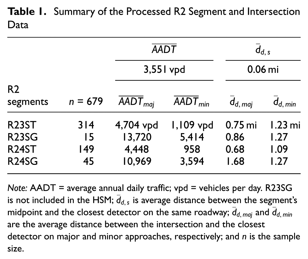
Note: AADT = average annual daily traffic; vpd = vehicles per day. R23SG is not included in the HSM; ${\bar{d}}_{d, s}$ is average distance between the segment’s midpoint and the closest detector on the same roadway; ${\bar{d}}_{d, maj}$ and ${\bar{d}}_{d, \min}$ are the average distance between the intersection and the closest detector on major and minor approaches, respectively; and n is the sample size.

It is important to note that assembling the final database of segments and intersections necessitates a substantial amount of data from various sources, and advanced programming skills to merge them into a single, usable database. Additionally, many data points that are not readily available need to be manually extracted, as done by many studies (e.g., 9 , 11 , 23 ), making the entire process cumbersome and prone to errors.

SPF Calibration

The functional form of Equation 4 is the focus of this section. It relates the total number of predicted crashes to the observed ones through a fixed parameter value. As discussed in the literature review section, while many studies have adopted Equation 4, others have explored different functional forms for C.

In this study, an ML-based method is employed to derive a more statistically robust estimate of C. This approach builds on the method introduced by Mehta and Lou ( 2 ), who estimated an NB model relating observed crash frequencies to the adjusted mean crash count (N_e), with C and α as model parameters. Rajabi et al. ( 4 ) later adopted the same framework but held α constant, using the default values provided in the HSM for each facility type. Expanding on Rajabi et al. ( 4 ), the current study additionally estimates the standard deviation of the ML-derived C, which is critical for calculating the CV and, in turn, for assessing whether the available sample size is adequate for reliable calibration.

Let us denote the observed crash data y_i for $i = 1, \dots, n$ facilities (either segments or intersections), along with the associated geometric and operational features. Let us also replace the notation N_spf,s in Equation 1 with ${\hat{μ}}_{i}^{b}$ as the expected crash frequency of facility i for the base conditions. Then denote ${\hat{μ}}_{i}^{a}$ as the expected crash frequency after adjusting for deviations from the base conditions by combining Equations 1 and 3 as ${\hat{μ}}_{i}^{a} = {\hat{μ}}_{i}^{b} K_{i}$ , where K_i is a constant term representing the product of CMFs for each facility i. The inherent motivation in using C is to alter the model coefficient a₀ in Equation 1 that would make ${\hat{μ}}^{a}$ close to y, as ${\hat{μ}}_{i}^{c} = C {\hat{μ}}_{i}^{b} K_{i}$ , where ${\hat{μ}}_{i}^{c}$ is the calibrated SPF. The intercept a₀ in Equation 1 becomes $a_{0} + \log (C)$ .

As the objective of a regression model is to determine the values of model coefficients that maximize the log-likelihood function given observed counts, as shown in Equation 8, one would find it natural to estimate C accordingly.

Let us assume for now that crash counts y follow Poisson distribution as $f (y; μ) = e^{- μ} μ^{y} / y!$ . The objective is to estimate ${\hat{μ}}^{c}$ as a function of C with its covariate ${\hat{μ}}^{b} K$ . Using data from n facilities, the log-likelihood function of C, given y, is $L (C; y) = \sum_{i = 1}^{n} - {\hat{μ}}_{i}^{c} + y_{i} \log ({\hat{μ}}_{i}^{c}) - \log (y_{i}!)$ . The ML estimate of C can then be found by:

\begin{matrix} \frac{d L (\hat{C}; y)}{dC} = \sum_{i = 1}^{n} s_{i} (\hat{C}; y) \\ = \sum_{i = 1}^{n} - \frac{d {\hat{μ}}_{i}^{c}}{dC} + y_{i} \frac{d \log ({\hat{μ}}_{i}^{c})}{dC} \\ = \sum_{i = 1}^{n} - {\hat{μ}}_{i}^{b} K_{i} + y_{i} \frac{{\hat{μ}}_{i}^{b} K_{i}}{{\hat{μ}}_{i}^{c}} = 0 \end{matrix}

(12)

where $s_{i} (\hat{C}; y)$ is the score, that is, the first derivative of the log-likelihood function for each i. Since, ${\hat{μ}}_{i}^{c} = \hat{C} {\hat{μ}}_{i}^{b} K_{i}$ , the value of $\hat{C}$ that satisfies this condition is $\hat{C} = \sum_{i = 1}^{n} y_{i} / \sum_{i = 1}^{n} {\hat{μ}}_{i}^{b} K_{i}$ or $\hat{C} = \sum_{i = 1}^{n} y_{i} / \sum_{i = 1}^{n} {\hat{μ}}_{i}^{a}$ . Note that this formulation for $\hat{C}$ is the same as Equation 4.

However, if we let y follow NB distribution (see Equation 7), as assumed in the HSM, then $\hat{C}$ that maximizes the log-likelihood shown in Equation 8 can be derived as:

\sum_{i = 1}^{n} \frac{α (y_{i} - C {\hat{μ}}_{i}^{a})}{C (α + C {\hat{μ}}_{i}^{a})} = 0

(13)

In this case, there is no closed form solution for finding $\hat{C}$ . Yet a simple root finder algorithm in any statistical software or in MS Excel™ can be used for this purpose, as done in Rajabi et al. ( 4 ).

Note that ML estimation of Equation 13 involves a single parameter, C, where α is held fixed at the reciprocal of the overdispersion parameter specified in the HSM for the facility type under consideration.

Table 2 shows the calibration factors for the R2 segments and intersections calculated by Equation 4 and the ones estimated using the ML-based method from Equation 13. Significant differences in the calibration factors are observed, especially for R23ST and R24ST facilities.

Table 2.

Comparison of Calibration Factors from Equations 4 and 13

Statistic	R2 Segments	R23ST	R24ST	R24SG
C (Equation 4)	1.506	0.861	0.842	0.817
Standard deviation (Bahar [ 18 ])	0.067	0.063	0.060	0.060
Standard deviation (Rajabi et al. [ 20 ])	0.091	0.056	0.073	0.080
$\hat{C}$ (Equation 13)	1.639	1.015	0.952	0.849
Standard deviation (Equation 14)	0.085	0.056	0.053	0.051
95% Confidence interval	[1.472, 1.806]	[0.905, 1.125]	[0.848,1.056]	[0.749,0.949]

The advantage of the ML-based method is that one can compute the standard error of $\hat{C}$ using the Fisher information as the expectation of the outer product of gradients, calculated as follows:

I = E [s_{i} (\hat{C}; y) s_{i} (\hat{C}; y)] = \frac{α {\hat{μ}}_{i}^{a}}{(α + \hat{C} {\hat{μ}}_{i}^{a}) \hat{C}}

(14)

ML estimate of C is unbiased, with a normal distribution. $\hat{C} ~ N (C, I^{- 1})$ as $n \to \infty$ . For only one parameter to be estimated I is a scalar, and the standard deviation of $\hat{C}$ is the square root of its reciprocal.

For example, for R2 segments $\hat{C}$ = 1.639 we compute I = 139.25 and its standard deviation is 0.085. Note that I is the expected information. If a standard optimization tool is used, one could directly use the negative of Hessian, that is, the observed information matrix, evaluated at the ML estimate. In this context, the Hessian is simply a scalar, the second derivative of the log-likelihood. In that case the standard error of $\hat{C}$ is the square root of this observed information matrix. Using this estimate, a 95% confidence interval for the parameter C is calculated and presented in the table.

Table 2 also compares the standard deviation for $\hat{C}$ with the ones for the traditional C, as per Equation 4, based on Bahar ( 18 ) and Rajabi et al. ( 20 )’s estimation using Equations 9 and 10, respectively.

Using the estimated C and standard deviations given in Table 2, the CV of each approach is also computed, as shown in Table 3.

Table 3.

Coefficient of Variation of Calibration Factors Estimated Using Different Methods

Statistic	R2 segments	R23ST	R24ST	R24SG
CV (Equation 9) of C (Equation 4)	0.044	0.073	0.071	0.073
CV (Equation 10) of C (Equation 4)	0.060	0.065	0.087	0.098
CV (Equation 14) of $\hat{C}$ (Equation 13)	0.052	0.055	0.056	0.060

The results indicate that, based on the assumption, as suggested by Bahar ( 18 ) that CV should fall within the range of 0.10 to 0.15, the sample sizes for each facility type are adequate.

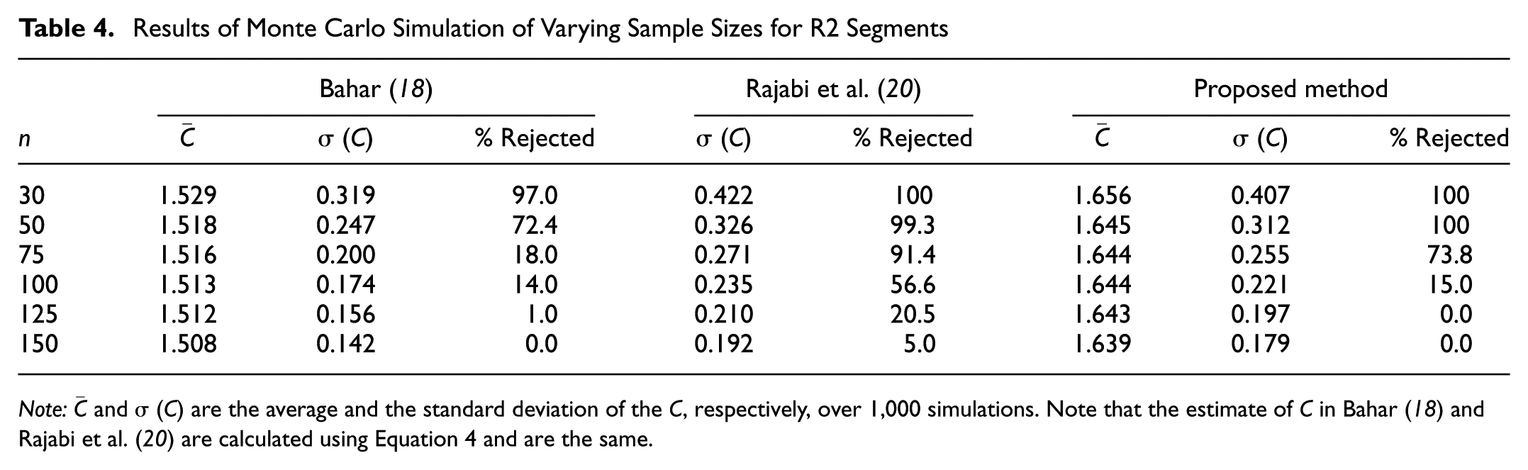
To evaluate the minimum sample size required for reliable calibration, a Monte Carlo simulation is performed, following the methodology used in Alluri et al. ( 15 ), Trieu et al. ( 16 ), and Shirazi et al. ( 19 ). The analysis focused on the R2 segment, which includes a total of 679 observations. The target values of parameter C were calculated as 1.506 and 1.639, based on Equations 4 and 13, respectively. Random samples of sizes 30, 50, 75, 100, 125, and 150 are drawn from the data set 1,000 times. For each iteration, the CV of the estimate is computed using the methods proposed by Bahar ( 18 ), Rajabi et al. ( 20 ), and the approach developed in this study, corresponding to Equations 9, 10, and 14, respectively. Table 4 presents the results, including the proportion of iterations in which the calculated CV outside the recommended range of 0.10 to 0.15 across 1,000 simulations.

Table 4.

Results of Monte Carlo Simulation of Varying Sample Sizes for R2 Segments

	Bahar ( 18 )			Rajabi et al. ( 20 )		Proposed method
n	$\bar{C}$	σ (C)	% Rejected	σ (C)	% Rejected	$\bar{C}$	σ (C)	% Rejected
30	1.529	0.319	97.0	0.422	100	1.656	0.407	100
50	1.518	0.247	72.4	0.326	99.3	1.645	0.312	100
75	1.516	0.200	18.0	0.271	91.4	1.644	0.255	73.8
100	1.513	0.174	14.0	0.235	56.6	1.644	0.221	15.0
125	1.512	0.156	1.0	0.210	20.5	1.643	0.197	0.0
150	1.508	0.142	0.0	0.192	5.0	1.639	0.179	0.0

Note: $\bar{C}$ and σ (C) are the average and the standard deviation of the C, respectively, over 1,000 simulations. Note that the estimate of C in Bahar ( 18 ) and Rajabi et al. ( 20 ) are calculated using Equation 4 and are the same.

The results indicate that although the estimate of C approaches its target value with a sample size of 30, the CV remains outside the recommended range for all three methods used to calculate its standard deviation. Based on Bahar’s ( 18 ) approach and the one proposed in this study, the proportion of iterations in which the CV exceeds the recommended range approaches an acceptable threshold of 5% when the sample size is between 100 and 125 for the facility under consideration. However, based on the approach by Rajabi et al. ( 20 ), the sample size that corresponds to a rejection of 5% is 150. This conservative number can be attributed to the CV estimated according to Equation 10 depending on the variance of the observed number of crashes.

Modeling Results of NJ Specific SPFs

The SPFs for R2 segments and intersections are developed using NB regression, as suggested by the HSM. The model estimation is performed in R statistical software. R23SG and R24SG models are not estimated because, as shown in Table 1, the number of data points is insufficient for GLM regression. The regression results are shown in Table 5, alongside the coefficients provided by the HSM. Note that β₀ is the intercept, and β₁ and β₂ are the coefficients for $\log (AADT)$ and $\log (L)$ for R2 segments, whereas for intersections, β₁ and β₂ are the coefficients for $\log (AAD T_{maj})$ and $\log (AAD T_{\min})$ .

Table 5.

NB Regression Results

Parameter	Estimate (SE)	z-value	HSM
R2 segments (1.88, 2.87)^‡
β₀	−6.731 (0.377)	−17.87^***	−8.23
β₁	0.875 (0.045)	19.59^***	1.0
β₂	0.954 (0.08)	12.00^***	1.0
α	2.147 (0.301)		L/0.236
Sample size = 679, logLik: −1,014.3, Pearson dispersion: 0.99, MAD: 1.34, LR ratio test: 0.20 (Sig.)
R23ST (4.84, 5.69)
β ₀	−6.987 (0.463)	−15.081^***	−9.86
β ₁	0.591 (0.058)	10.179^***	0.79
β ₂	0.297 (0.047)	6.366^***	0.49
α	2.713 (0.376)		1.852
Sample size = 314, logLik: −735.34, Pearson dispersion: 0.989, MAD: 2.81, LR ratio test: 0.88 (Sig.)
R24ST (7.58, 7.86)
β ₀	−5.950 (0.647)	−9.206^***	−8.56
β ₁	0.350 (0.072)	4.973^***	0.60
β ₂	0.512 (0.071)	7.217^***	0.61
α	2.388 (0.389)		4.17
Sample size = 149, logLik: −417.85, Pearson dispersion: 1.151, MAD: 4.27, LR ratio test: 0.80 (Sig.)

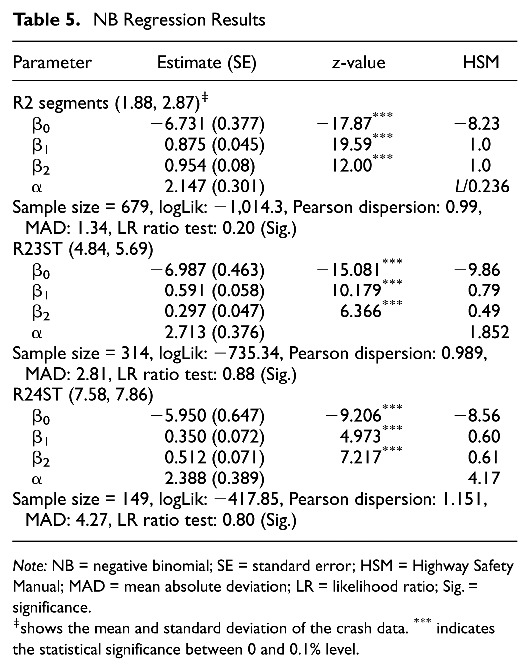
Note: NB = negative binomial; SE = standard error; HSM = Highway Safety Manual; MAD = mean absolute deviation; LR = likelihood ratio; Sig. = significance.

‡

shows the mean and standard deviation of the crash data. ^*** indicates the statistical significance between 0 and 0.1% level.

The table also presents various model statistics including:

(1) Pearson dispersion statistic, defined as $(\sum_{i = 1}^{n} {(y_{i} - {\hat{μ}}_{i})}^{2} / var ({\hat{μ}}_{i})) / (n - p)$ , where p is the number of model parameters,

(2) Mean absolute deviation (MAD), defined as $(\sum_{i = 1}^{n} | y_{i} - {\hat{μ}}_{i} |) / n$ ,

(3) Likelihood ratio (LR) Test, in which the developed NB model is compared with an intercept-only model using a likelihood ratio test. The traditional likelihood ratio test is defined as $LR = - 2 (L_{R} - L_{F})$ where $L_{F}$ is the log-likelihood for the model and $L_{R}$ is the log-likelihood for the intercept-only model. LR is treated as a chi-square random variate. Here, the full model uses two covariates in addition to the intercept; the degrees of freedom for the chi-square test are, therefore, two.

Note that the number of years (5) is included in the regression model as an offset. Various combinations of covariates were tested, and traffic volume and segment length consistently emerged as statistically significant predictors, along with pavement width in R2 segments and skew angle in R23ST. However, the inclusion of these variables does not significantly improve the model statistics. Therefore, these two covariates are excluded from Table 5 to facilitate ease of understanding and comparison with the HSM coefficients, which are also included in the table as a reference.

As seen in Table 5, for all models the Pearson dispersion statistic is very close to 1.0, indicating that the NB model can handle the overdispersion inherent in the crash data. MAD statistics are 1.34, 2.81, and 4.27 for R2 segments, R23ST, and R24ST, respectively, indicating how much the estimated mean differs from the observed crash count on average. This statistic is commonly used in the literature (e.g., 4 , 37 , 43 ) to measure the accuracy of the calibrated or the developed SPFs or when comparing these two approaches. For example, using the calibrated SPFs in accordance with Equation 4, the MAD statistics were computed as 1.36, 2.78, and 4.37 for the same facilities; and in accordance with Equation 13, they were 1.40, 3.09, and 4.68. The minor differences between these values make it challenging for an analyst to determine which model fits the data better. In addition, as mentioned in Bartin et al. ( 17 ), this approach disregards the probabilistic nature of crash occurrence. The difference between the predicted crash count and its observed value is incomplete information without considering the variance of crashes at that location.

Comparison of Calibrated and Developed SPFs

To compare the calibrated and developed SPFs, three methods are used: the LR ratio test, the Rootogram plots ( 44 ), and chi-square test.

As shown in Table 5, according to the LR test, all models are significant compared with the intercept-only model. But this is usually the case as most models fit better than an intercept-only model even when both fail to fit the data ( 6 ). The log-likelihood of the calibrated SPFs are computed as −1,026.61, −738.03, and −410.47. Comparing with the log-likelihood values of the estimated models shown in Table 5, a 2 degree-of-freedom chi-square test results in p-values of 0.99, 0.93, and 0.99 for R2 segments, R23ST, and R24ST, respectively, indicating that the developed NB models are a significantly better fit to the crash data compared with the calibrated SPFs.

Figure 2 shows the Rootogram plots for the developed and calibrated SPFs (in accordance with Equation 4) that compare the observed and expected counts graphically by plotting histogram-like rectangles for the observed frequencies and a curve for the theoretical fit (represented by a red line). Note that the x-axis in these figures shows 95% of the observed crash counts for each facility, with the last bin representing the remaining 5%.

For R2 segments, although the MAD statistics were very close, the Rootograms indicate that the developed SPFs yield better crash frequency predictions, especially at zero crashes. A similar trend is also observed for R23ST and R24ST. Nevertheless, it might not be clear, as in R24ST case, how to determine which model fits better by visual inspection alone. Pearson’s chi-square test could provide a quick assessment for this purpose, where a lower test statistic indicates a better fit between observed and predicted values.

The chi-square values for the calibrated SPFs in accordance with Equation 4 are computed as 29.3, 31.9, and 24.5 for R2 segments, R23ST, and R24ST, respectively; whereas when calibrated based on Equation 13, the chi-square values for the calibrated SPFs are computed as 25.9, 27.2, and 21.3, indicating a relatively better fit than the traditional calibration method. On the other hand, the values computed for the developed SPFs are 12.7, 5.9, and 18.8, showing a significantly better match between the observed and predicted crash counts.

It should be noted that these chi-square values can only be used to assign a numerical value to the Rootograms and for comparison purposes, but not as a formal test statistic, since they fail to control for estimation error. For a more formal test, such as conditional moments test, readers are referred to Cameron and Trivedi ( 45 ).

Discussion on Challenges and Considerations in Calibrating and Developing Safety Performance Functions

There have been many studies conducted since the first edition of the HSM in 2010. It is expected that many other state DOTs will seek to calibrate HSM SPFs or develop jurisdiction-specific ones, or update the existing ones as new data become available. It is, therefore, important to elaborate on the strategic direction state agencies should take when considering the findings. Numerous studies have focused solely on calibration or development, or both, yet the choice of whether to calibrate the HSM SPFs or develop state-specific SPFs is not extensively discussed. This decision involves trade-offs, including sample size, data processing, labor, and the accuracy of estimates.

One of the HSM’s guidelines suggests that the new SPFs: (a) should use facility data with the same base conditions used in the manual, or (b) should be capable of being converted to those base conditions ( 1 ). Choosing option (a) is nearly improbable because it filters out a large portion of the acquired data set and makes it insufficient for statistically significant regression results. Option (b) suggests including all covariates in the model and replacing them with the base condition values to convert them to the general forms shown in Equation 1 or 2. This option raises several questions. For instance, if a variable, say lighting, comes out significant, should the analyst suppress its coefficient and use the CMF suggested by the HSM? What if the sign of its coefficient is the opposite from what is expected? What if some or all other variables come out statistically insignificant? Should the analyst still replace them with the base values and use the CMFs or repeat the regression analyses without these variables? These questions, along with the one on whether to calibrate or develop SPFs, should be answered in close coordination and communication with the safety practitioners who will eventually make use of the results. As also stated in Srinivasan and Carter ( 38 ) the future applications of the developed SPFs should be considered in this decision process.

Interviews with the New Jersey DOT safety practitioners revealed that they are required to use the HSM’s application spreadsheets for safety analyses. Modifying these with newly developed SPFs, especially those with covariates different from the HSM, is viewed as a major hurdle. Thus, using calibration factors appears more straightforward. However, calibration factors and developed SPFs are subject to change and need to be updated as new data sets become available. For example, the calibration factors shown in Table 2 were based on crash data from 2011 to 2015. When the crash data from 2016 and 2017 were used, the calibration factors were computed as 1.556, 0.851, 1.068, and 0.992 for R2 segments, R23ST, R24ST, and R24SG, respectively. While the calibration factors for the first two facilities are close to the ones shown in Table 2, the ones for R24ST and R24SG are significantly higher compared with those previously computed (0.842, 0.817). This shows the need for constantly updating these values as new data become available. Nevertheless, this process requires advanced statistical and data mining skills, suggesting that a computerized tool to automatically update results would be highly beneficial for state agencies.

The process of calibrating and developing SPFs involves considerable time, effort, and resources, requiring detailed data from various sources. Identifying all readily available data sources and automating data gathering can alleviate some of the burden, but manual extraction is often inevitable, particularly for geometry and operational characteristics data. For example, horizontal curvature data is rarely available in state roadway inventory databases. Studies have either assumed default values for horizontal curvature CMFs or omitted sections with horizontal curvature (e.g., 8 , 15 , 37 ) or manually extracted this information using Google Earth (e.g., 23 , 35 ) or built-in plans (e.g., 8 , 10 ). However, the accuracy of manually extracted data can be questionable. Bartin et al. ( 42 ) found significant variability and low correct detection rates in manually extracted horizontal curvature data, suggesting the need for novel methods to extract data automatically. Other novel methods can be used to get large-scale reliable estimates of required and desirable data, such as the number of left-turn and right turn lanes, the presence of lighting, parking information, presence of schools, and so forth. For example, Yin et al. ( 46 ) investigated the feasibility of using machine learning methods to detect and count pedestrians from Google Street View images, with estimation results reported to be within a reasonable level of accuracy compared with observed pedestrian counts. Similarly, Campbell et al. ( 47 ) explored the use of deep learning to produce an autonomous system for detecting traffic signs on Google™ Street View images, showing that the process is scalable with a detection accuracy of 95.63% and classification accuracy of 97.82%. In addition, Yang and Das ( 48 ) used publicly available United States Geological Survey digital elevation model data to develop an open-source program to extract horizontal and vertical alignment information for roadways, leveraging public data and open application programming interfaces.

Aside from geometry and operational data, AADT and crash frequency data are also crucial. Although state DOTs conduct comprehensive traffic count programs, available AADT data sets often fall short of the HSM’s requirements. Milligan et al. ( 49 ) reported that short-term count length plays a major role in AADT estimation errors, varying from 8.7% to 17.1%. El-Basyouny and Sayed ( 50 ) showed that when the errors in AADT were significant, SPFs underestimated the predicted number of crashes in the presence of heavy traffic, especially for long road segments. For intersections, especially in rural areas, the lack of minor AADT data is a more common issue, often addressed by statistical models or interpolation ( 11 ). The accuracy of AADT data affects calibration and development results, but this has received little attention in the literature.

The accuracy of crash data is another critical factor. Studies have noted the impact of the crash reporting threshold on the scale of the calibration factors (e.g., 12 , 23 , 37 ). Crash data from various states were used in developing the HSM predictive models, and any deviation from the baseline crash reporting threshold would affect the estimation results for property damage crashes. Yet little attention is paid in the literature to the discussion on how the incorrect crash frequency data variables can affect the calibration or development results. For example, as seen in Equation 4, inaccuracies in the observed crash frequency would directly affect the calibration factors. In fact, the results presented in the previous section are based on the latest crash frequency data obtained from the New Jersey DOT in 2019, which is significantly different from its previous version. As mentioned before, the crash location, although crucial, is the most incomplete part of the crash database, in which some of the location information such roadway SRI, milepost, direction, or crash coordinates are often missing. As a result, the New Jersey DOT post-processes the raw crash data and geocodes crashes with missing coordinates using SRI, milepost, and cross street names. In 2019, the New Jersey DOT updated its post-processing procedure based on a tighter threshold used in geocoding process to increase the accuracy of crash coordinates, which resulted in 14.7% fewer crashes statewide, compared with the previous version. To demonstrate how this would have changed the calibration factors in retrospect, the calibration process is repeated with the previous version of the crash database for the years 2011 to 2015. The calibration factor for R2 segments is calculated as 1.82 (20.8% increase), and for R23ST, R24ST, and R24SG, they are calculated as 0.90 (4.5% increase), 0.96 (14.0% increase), and 0.92 (12.6% increase), respectively.

Conclusions

This paper focused on the calibration and development of SPFs, using R2 segments and intersections in NJ as a case study. As part of this scope, the details of the data processing and extraction efforts necessary for crash frequency prediction models were presented. It was emphasized that assembling the necessary data, whether for calibration or development, involves rigorous tasks of compiling, cleaning, and processing, and requires substantial computer programming effort. An alternative method for estimating the calibration factor using ML estimation, proposed in the literature by Mehta and Lou ( 2 ) and Rajabi et al. ( 4 ) was extended, allowing for the estimation of the standard error of the calibration factor. The results indicated significant differences in calibration factors when estimated using these two different methods (Table 2). The CV of the estimated C was then calculated and compared with the ones estimated as proposed by Bahar ( 18 ) and Rajabi et al. ( 20 ) and presented in Table 3. A Monte Carlo simulation was conducted to evaluate and compare the minimum sample size required for reliable calibration using the available methods for calculating CV (Table 4).

In addition, the results of modeling NJ-specific SPFs were presented, along with various model statistics (Table 5). The comparison of the calibrated and the newly developed SPFs were conducted using a log-likelihood ratio test, Rootogram plots (Figure 2), and chi-square test.

In addition, through past literature and best practices, this paper also discussed the practicality of the current manual data extraction practices and argued that novel data extraction methods should be adopted to minimize labor-intensive and cost-prohibitive manual data collection processes and increase data accuracy. Finally, the importance of the accuracy of crash location was underlined, the deviations in calibration factors were reported with changes to crash locations. Similar inaccuracies with crash locations are expected in other states’ crash databases, and therefore their potential impact on the calibration and development results should be recognized in future studies. One should, therefore, be cognizant of the efforts being made to manually extract the required roadway geometry and operational features data not included in available data repositories can easily be offset by the inaccuracies in crash databases.

Footnotes

Author Contributions

The authors confirm contribution to the paper as follows: study conception and design: Bekir Bartin, Kaan Ozbay; data collection: Bekir Bartin, Kaan Ozbay; analysis and interpretation of results: Bekir Bartin, Kaan Ozbay; draft manuscript preparation: Bekir Bartin, Kaan Ozbay. All authors reviewed the results and approved the final version of the manuscript.

Declaration of Conflicting Interests

The authors declared no potential conflicts of interest with respect to the research, authorship, and/or publication of this article.

Funding

The authors disclosed receipt of the following financial support for the research, authorship, and/or publication of this article: The study is supported by the New Jersey DOT (FHWA-NJ-2019-007) and partially by C2SMARTER, a Tier 1 UTC at New York University funded by the U.S. DOT, and Ozyegin University.

ORCID iDs

Bekir Bartin

Kaan Ozbay

The contents of this paper reflect the views of the authors only, who are responsible for the facts presented and do not represent any official views of the sponsoring organizations or agencies.

References

American Association of State Highway and Transportation Officials. Highway Safety Manual. Washington, DC, 2010, 529.

Mehta

Lou

Calibration and Development of Safety Performance Functions for Alabama: Two-Lane, Two-Way Rural Roads and Four-Lane Divided Highways. Transportation Research Record: Journal of the Transportation Research Board, 2013. 2398: 75–82.

Hull

Wemple

Fish

Silverman

K. K.

Perez-Bravo

State Policies and Procedures on Use of the Highway Safety Manual. Report No. FHWA-SA-16-119. Washington, DC, 2016.

Rajabi

Ogle

J. H.

Gerard

Highway Safety Manual Calibration: Assessing Alternate Definitions of the Calibration Factor. Transportation Research Record: Journal of the Transportation Research Board, 2018. 2672: 99–108.

McCullagh

Nelder

J. A.

Generalized Linear Models. London: Chapman & Hall/CRC, 1989.

Hilbe

J. M.

Modeling Count Data. Cambridge: Cambridge University Press, 2014.

Ozbay

Nassif

Bartin

Bhattacharyya

Calibration/Development of Safety Performance Functions for New Jersey. FHWA-NJ-2019-007. New Jersey Department of Transportation, Trenton, NJ; Federal Highway Administration, U.S. Department of Transportation, Washington, D.C., 2019.

Sun

Brown

Edara

Carlos

Nam

Calibration of the Highway Safety Manual for Missouri. Report No. MATC-MU: 177. Mid-America Transportation Center, 2013.

Sun

Magri

Shirazi

H. H.

Application of the Highway Safety Manual Draft Chapter: Louisiana Experience. Transportation Research Record: Journal of the Transportation Research Board, 2006. 1950: 55–64.

10.

Lubliner

Bornheimer

Schrock

Wang

M. H.

Fitzsimmons

Evaluation of Interactive Highway Safety Design Model Crash Prediction Tools for Two-Lane Rural Roads on Kansas Department of Transportation Projects. Kansas Department of Transportation, 2014.

11.

Xie

Gladhill

Dixon

K. K.

Monsere

C. M.

Calibration of Highway Safety Manual Predictive Models for Oregon State Highways. Transportation Research Record: Journal of the Transportation Research Board, 2011. 2241: 19–28.

12.

Jalayer

LaMondia

J. J.

Williamson

Zhou

Developing Calibration Factors for Crash Prediction Models with Consideration of Crash Recording Threshold Change. Transportation Research Record: Journal of the Transportation Research Board, 2015. 2515: 57–62.

13.

Saha

Alluri

Gan

A Bayesian Procedure for Evaluating the Frequency of Calibration Factor Updates in Highway Safety Manual (HSM) Applications. Accident Analysis and Prevention, Vol. 98, 2017, pp. 74–86.

14.

Banihashemi

Sensitivity Analysis of Data Set Sizes for Highway Safety Manual Calibration Factors. Transportation Research Record: Journal of the Transportation Research Board, 2012. 2279: 75–81.

15.

Alluri

Saha

Gan

Minimum Sample Sizes for Estimating Reliable Highway Safety Manual (HSM) Calibration Factors. Journal of Transportation Safety and Security, Vol. 8, No. 1, 2016, pp. 56–74.

16.

Trieu

Park

McFadden

Use of Monte Carlo Simulation for a Sensitivity Analysis of Highway Safety Manual Calibration Factors. Transportation Research Record: Journal of the Transportation Research Board, 2014. 2435: 1–10.

17.

Bartin

Ozbay

Safety Performance Functions for Two-Lane Urban Arterial Segments. Safety Science, Vol. 167, 2023, p. 106284.

18.

Bahar

User's Guide to Develop Highway Safety Manual Safety Performance Function Calibration Factors. National Cooperative Highway Research Program, Transportation Research Board, Washington, DC, 2014.

19.

Shirazi

Lord

Geedipally

S. R.

Sample-Size Guidelines for Recalibrating Crash Prediction Models: Recommendations for the Highway Safety Manual. Accident Analysis and Prevention, Vol. 93, 2016, pp. 160–168.

20.

Rajabi

Gerard

Ogle

Highway Safety Manual Calibration: Estimating the Minimum Required Sample Size. Transportation Research Record: Journal of the Transportation Research Board, 2022. 2676: 510–523.

21.

Geedipally

S. R.

Shirazi

Lord

Exploring the Need for Region-Specific Calibration Factors. Transportation Research Record: Journal of the Transportation Research Board, 2017. 2636: 73–79.

22.

Llopis-Castelló

Findley

D. J.

Influence of Calibration Factors on Crash Prediction on Rural Two-Lane, Two-Way Roadway Segments. Journal of Transportation Engineering, Vol. 145, No. 6, 2019, pp. 04019024-1–04019029.

23.

Shin

Lee

Y. J.

Dadvar

The Development of Local Calibration Factors for Implementing the Highway Safety Manual in Maryland. Office of Traffic and Safety (OOTS), Maryland State Highway Administration, Publication SP209B4J, 2014.

24.

Srinivasan

Haas

Dhakar

Hormel

Torbic

Harwood

Development and Calibration of Highway Safety Manual Equations for Florida Conditions. 2011.

25.

Troyer

Bradbury

Juliano

Strength of the Variable Calculating and Evaluating Safety Performance Function Calibration Factors for the State of Ohio. Transportation Research Record: Journal of the Transportation Research Board, 2018. 2515: 86–93.

26.

Srinivasan

Colety

Bahar

Crowther

Farmen

Estimation of Calibration Functions for Predicting Crashes on Rural Two-Lane Roads in Arizona. Transportation Research Record: Journal of the Transportation Research Board, 2016. 2583: 17–24.

27.

Matarage

I. C.

Dissanayake

Quality Assessment Between Calibrated Highway Safety Manual Safety Performance Functions and Calibration Functions for Predicting Crashes on Freeway Facilities. Journal of Traffic and Transportation Engineering (English Edition), Vol. 7, No. 1, 2020, pp. 76–87.

28.

Shirazi

Geedipally

S. R.

A Simulation Analysis to Explore When Using a Calibration Function Is Preferred over a Scalar Factor for Calibrating Safety Performance Functions. Journal of Transportation Safety and Security, Vol. 15, No. 4, 2022, pp. 335–349.

29.

Claros

Sun

Edara

HSM Calibration Factor, Calibration Function, or Jurisdiction-Specific Safety Model – A Comparative Analysis. Journal of Transportation Safety and Security, Vol. 12, No. 2, 2020, pp. 309–328.

30.

Son Oh

Kwon

Park

Abdel-Aty

Applying an Improved Calibration Method in the Safety Evaluation Framework for the Open Tolling System. Transportmetrica A: Transport Science, 2023, pp. 1–14.

31.

Garber

N. J.

Rivera

Safety Performance Functions for Intersections on Highways Maintained by the Virginia Department of Transportation. Virginia Department of Transportation Research Report, Report No. FHWA/VTRC 11-CR1, 2010.

32.

Garber

N. J.

Haas

P. R.

Gosse

Development of Safety Performance Functions for Two-Lane Roads Maintained by the Virginia Department of Transportation. Virginia Department of Transportation Research Report, Report No. FHWA/VTRC 10-R25, 2010.

33.

Shankar

Madanat

Methods for Identifying High Collision Concentrations for Identifying Potential Safety Improvements: Development of Safety Performance Functions for California. California Department of Transportation Research Report, Report No. CA15-2317, 2015.

34.

Kweon

Y. J.

Lim

I. K.

Development of Safety Performance Functions for Multilane Highway and Freeway Segments Maintained by the Virginia Department of Transportation. Report No. FHWA/VCTIR 14-R14. Virginia Center for Transportation Innovation and Research, 2014.

35.

Savolainen

P. T.

Gates

Lord

Geedipally

Rista

Barrette

Russo

B. J.

Hamzeie

Michigan Urban Trunkline Intersections Safety Performance Functions (SPFs) Development and Support. Michigan Department of Transportation Research Report, Report No. RC-1628, 2015.

36.

Donnell

Gayah

Jovanis

Safety Performance Functions. Pennsylvania Department of Transportation Research Report, Report No. FHWA-PA-2014-007-PSU WO 1, 2014.

37.

Donnell

Gayah

Regionalized Safety Performance Functions. Pennsylvania Department of Transportation Research Report, Report No. FHWA-PA-2016-001-PSU WO 017, 2016.

38.

Srinivasan

Carter

D. L.

Development of Safety Performance Functions for North Carolina. North Carolina Department of Transportation, Research and Analysis Group, Chapel Hill, NC, 2011.

39.

Hauer

Bamfo

Two Tools for Finding What Function Links the Dependent Variable to the Explanatory Variables. Proceedings of the International Cooperation on Theories and Concepts in Traffic safety (ICTCT) 1997 Conference, Lund, Sweden, 1997, pp. 1–19.

40.

New Jersey Geographic Information Network. New Jersey Geographic Information Network Website. https://njgin.nj.gov/njgin/about/gin. Accessed July 5, 2024.

41.

Bartin

Demiroluk

Ozbay

Jami

Automatic Identification of Roadway Horizontal Alignment Information Using Geographic Information System Data: CurvS Tool. Transportation Research Record: Journal of the Transportation Research Board, 2022. 2676: 532–543.

42.

Bartin

Ozbay

Extracting Horizontal Curvature Data from GIS Maps: Clustering Method. Transportation Research Record: Journal of the Transportation Research Board, 2019. 2673: 264–275.

43.

Lyon

Persaud

Gross

The Calibrator: An SPF Calibration and Assessment Tool User Guide. FHWA-SA-17-016, 2016.

44.

Kleiber

Zeileis

Visualizing Count Data Regressions Using Rootograms. The American Statistician, Vol. 70, No. 3, 2016, pp. 296–303.

45.

Cameron

A. C.

Trivedi

P. K.

Regression Analysis of Count Data. 2nd ed. Cambridge University Press, 2013.

46.

Yin

Cheng

Wang

Shaod

Big Data for Pedestrian Volume: Exploring the Use of Google Street View Images for Pedestrian Counts. Applied Geography, Vol. 63, 2015, pp. 337–345.

47.

Campbell

Both

Sun

(Chayn). “Detecting and Mapping Traffic Signs from Google Street View Images Using Deep Learning and GIS.” Computers, Environment and Urban Systems, Vol. 77, 2019, Article 101350.

48.

Yang

Das

Efficient Extraction of Horizontal and Vertical Alignment Information for Roadways Using Public Data and Open Application Programming Interfaces. Transportation Research Record: Journal of the Transportation Research Board, 2024. 2678: 2046–2058.

49.

Milligan

Montufar

Regehr

Ghanney

Road Safety Performance Measures and AADT Uncertainty from Short-Term Counts. Accident Analysis and Prevention, Vol. 97, 2016, pp. 186–196.

50.

El-Basyouny

Sayed

Safety Performance Functions with Measurement Errors in Traffic Volume. Safety Science, Vol. 48, No. 10, 2010, pp. 1339–1344.