Enhancing Wind Field Prediction and Reconstruction around Windbreak Walls along High-Speed Railway by Advanced Neural Network Architectures: Accuracy and Stability Assessment

Abstract

Accurate prediction of wind fields around high-speed railway (HSR) infrastructure is critical for operational safety and energy efficiency. This study evaluates neural network approaches for predicting wind fields around HSR windbreak walls, focusing on transformer models. Field measurements were conducted using 15 anemometer masts arranged inside and outside windbreak walls on the Lanzhou–Xinjiang railway. We compared multiple deep learning architectures (multilayer perceptron, long-short-term memory, temporal convolutional network and transformer) for predicting interior wind conditions based on exterior measurements. The key findings are summarized as follows: (1) prediction accuracy improved substantially with longer historical contexts (10–60 timesteps); (2) significant spatial variability exists in wind predictability across measurement locations; (3) feature importance analysis identified critical measurement points, enabling cost-effective maintenance strategies and optimized sensor deployment; and (4) sequence mean filling performed best among the three tested strategies for handling missing data, maintaining positive predictive power even with substantial sensor loss. Among these models, the transformer model achieved the best overall performance (R² = 0.9665 at T = 60), with its advantage becoming most pronounced at longer historical contexts. These findings have important implications for railway safety and wind energy applications, enabling more efficient monitoring networks and robust forecasting systems. The demonstrated effectiveness of transformer models represent a significant advancement in applying attention-based architectures to infrastructure monitoring challenges.

Keywords

high-speed railway wind speed prediction machine learning transformer signal processing

Introduction

Renewable energy sources, particularly wind energy, have gained significant attention over the past decades because of increasing environmental concerns and energy demand ( 1 , 2 ). The accurate and reliable forecasting of wind conditions is essential for wind power integration, energy management optimization, and infrastructure safety ( 3 , 4 ). In China, the rapid development of high-speed railways (HSRs) has posed new requirements and challenges to accurately forecasting wind fields along railway lines (5 –8). Strong winds adversely affect HSR operations by increasing aerodynamic forces and structural vibrations on trains, severely compromising passenger comfort and safety. To mitigate potential hazards, wind barriers have been widely constructed on HSR lines, dividing local areas into the internal (trackside, sheltered by barriers) and external (outside barriers, unsheltered) regions ( 9 , 10 ).

In current practice, monitoring wind conditions along railway routes typically requires intensive installation of wind sensors on both sides of wind barriers. While measurement equipment inside barriers ensures accuracy in railway operation safety monitoring, dense sensor deployments significantly increase equipment investment, data redundancy, and maintenance complexity (11 –13). Therefore, developing data-driven methodologies to predict internal wind conditions from external field measurements represents a critical opportunity to minimize operational costs without sacrificing safety performance ( 14 , 15 ).

Recent advances in deep learning have revolutionized time series forecasting capabilities across various domains (16 –19). Among emerging architectures, the transformer model, initially developed for natural language processing tasks ( 20 ), has demonstrated remarkable potential for capturing complex temporal dependencies in sequential data. Unlike traditional recurrent neural networks that process data sequentially, the transformer’s self-attention mechanism enables parallel computation and more effective modeling of long-range dependencies, making it particularly suitable for nonstationary time series such as wind speed data (21 –25). Despite these advantages, transformer models remain less commonly applied in energy-related forecasting applications, especially in complex engineering environments such as railway wind barriers ( 18 , 26 , 27 ).

This study investigates the application of transformer models for predicting wind fields around HSR windbreak structures, with implications extending to wind energy systems and broader energy applications. We present a comprehensive comparison of the transformer architecture against established baseline models including multilayer perceptron (MLP), long-short-term memory (LSTM) ( 28 ), temporal convolutional network (TCN) ( 29 ), and neural basis expansion analysis for time series (N-BEATS) ( 30 ). The research evaluates these models across several key dimensions: prediction accuracy under varying historical context lengths, spatial generalization capabilities across different measurement locations, feature importance patterns, and resilience to missing input features—a critical concern for operational energy and transportation systems. The key contributions of this work include:

The demonstration of transformer architecture superiority for wind field prediction with potential applications in both transportation and energy sectors.

Identification of spatial variation in predictability across different measurement locations.

Examination of feature importance dynamics revealing a clear measurement point hierarchy, enabling prioritized maintenance strategies and optimized sensor placement for future projects.

Evaluation of missing data handling strategies to enhance operational robustness in real-world deployment scenarios.

The remainder of this paper is organized into sections as follows: a presentation of the field experiment setup, data acquisition process, and preprocessing methods; details the architectural design of the baseline models (MLP, LSTM, TCN, N-BEATS) and the proposed transformer model; the provision of comprehensive analysis of experimental results, including comparative prediction performance evaluation; a discussion the practical implications and limitations; and finally, a summary the key findings and suggests directions for future research.

Data Acquisition and Preprocessing

Experimental Design

The experimental site was located at a critical section of the Lanzhou–Xinjiang HSR where a significant train swaying phenomenon had been previously reported under strong wind conditions. This section was specifically selected because of its historical wind-related operational challenges and recent windbreak wall modifications designed to reduce crosswind effects on passing trains. The windbreak wall along this section has a constant height of 3.5 m throughout the measurement region. The measurement system used in this study is an existing wind monitoring network deployed by the railway authority along this section, rather than a setup designed for this research. The mast positions and heights were determined by the operator according to operational monitoring needs and onsite constraints, including the safe-clearance requirement of the overhead contact system on the trackside and the conventional reference height for incoming-flow monitoring on the windward side. The wind field measurement system consisted of 15 anemometer masts arranged to capture comprehensive wind data both inside and outside the windbreak walls. Nine masts (numbered #1 to #9) were installed inside the windbreak walls near the railway tracks, while six masts (#10 to #15) were placed outside the walls on the windward side to measure the incoming wind conditions. The positioning of the measurement masts followed an arrangement to ensure coverage of the railway wind field for monitoring, as shown in Figure 1. Within the protected zone, Masts 1# to #7 were positioned 2.5 m from the centerline of the up track. Mast #8 was placed between the uptrack and downtrack at 2.5 m from each track’s centerline, while Mast #9 was situated 2.5 m from the centerline of the downtrack. The distance between two lines is 5 m. For enhanced vertical profiling, Masts #4, #8, and #9 were equipped with three pairs of wind speed and direction sensors at heights of 2 m, 3 m, and 4 m above the track surface. The remaining interior masts had single sensor pairs installed at 2.3 m height. The exterior masts (#10 to #15) were each equipped with a pair of wind speed and direction sensors at 4 m above ground level. The 4 m height for external masts captures the environmental inflow. The 2 m, 3 m, and 4 m sensors on Masts #4, #8, and #9 are used to resolve the vertical wind profile behind the wall, while the remaining 2.3 m single-sensor masts target the train-body level. For internal measurements, sensor heights were restricted to 2.3 m to maintain safety clearance from the overhead contact system. This position corresponds to the upper-middle section of the train body, offering a direct measurement of the lateral wind forces affecting the vehicle.

Figure 1.

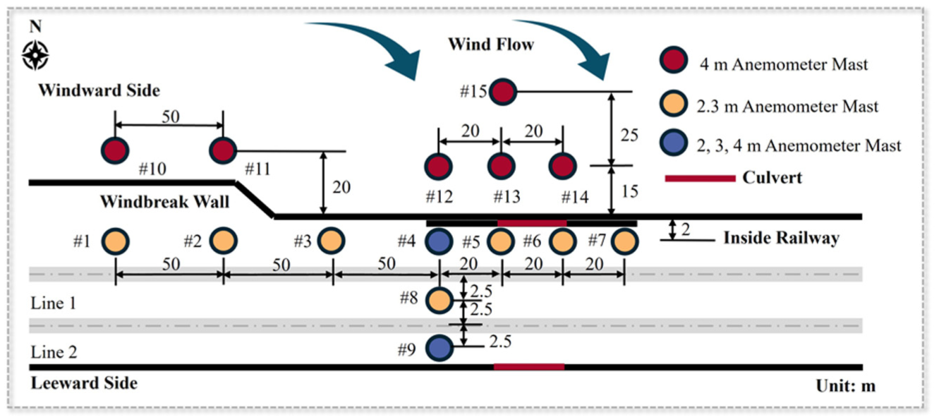
Top-view schematic diagram of anemometer mast arrangement and windbreak wall position.

Data Preprocessing

The field measurements were conducted over a continuous 4-h period under no-train-passage conditions. This time window was selected based on meteorological forecasts predicting strong winds characteristic of the region’s typical challenging conditions. The measurements captured wind speed and direction data with high temporal resolution, providing a detailed characterization of wind behavior around the windbreak structure. The raw data collected included instantaneous wind speeds at each sensor location.

The raw wind data were initially collected at a high sampling frequency of 180 Hz. To facilitate effective modeling while preserving essential wind dynamics, we downsampled the data to 1 Hz by computing 1 s average values of wind speed. All wind speed measurements underwent min–max normalization to the [0, 1] range to improve neural network training stability. For model development, we structured the data to reflect the physical relationship between outside and inside wind conditions. Input features comprised measurements from the exterior masts (#10–#15) positioned outside the windbreak walls, while target outputs were the corresponding wind speeds from interior masts (#1, #2, #3, #4-4, #4-3, #4-2, #5, #6), where the notation #4-4, #4-3, and #4-2 represents sensors at Mast #4 positioned at heights of 4 m, 3 m, and 2 m respectively. To generate the specific training samples, we employed a sliding window approach with a stride of 1 s. In this context, the input sequence length T corresponds to the number of tokens; we constructed three distinct experimental datasets with input histories of T = 10-, 30-, and 60-time steps, while fixing the prediction horizon at S = 10. The dataset was partitioned with 80% allocated for model training and 20% for testing, maintaining the temporal sequence integrity essential for time series forecasting applications.

Neural Network Model Construction

Problem Definition

The wind field prediction problem can be formalized as a multivariate time series forecasting task where we aim to predict wind speeds at multiple interior positions based on historical observations from exterior measurement points. Let $X_{t}^{ext} \in R^{m}$ represent the wind measurements from m exterior anemometer masts at time step t, and $Y_{t}^{int} \in R^{n}$ denote the corresponding measurements from n interior masts behind the windbreak wall. Our objective is to develop models that learn the mapping function f such that

Y_{t : t + s}^{int} = f (X_{t - T : t - 1}^{ext})

(1)

where $X_{t - T : t - 1}^{ext}$ represents the sequence of exterior wind measurements over a window of T previous time steps and s is the prediction step length. In this study, we set T = 60 and S = 10.

Input variables consist of normalized wind speed and direction measurements from exterior masts (#10–#15), while output variables include the wind speeds from interior masts (#1, #2, #3, #4-4, #4-3, #4-2, #5, #6). The prediction accuracy is evaluated using multiple metrics including mean absolute error (MAE), root mean square error (RMSE), and coefficient of determination (R²), which are defined as

MAE = \frac{1}{N} \sum_{i = 1}^{N} | y_{i} - {\hat{y}}_{i} |

(2)

RMSE = \sqrt{\frac{1}{N} \sum_{i = 1}^{N} {(y_{i} - {\hat{y}}_{i})}^{2}}

(3)

R^{2} = 1 - \frac{\sum_{i = 1}^{N} {(y_{i} - {\hat{y}}_{i})}^{2}}{\sum_{i = 1}^{N} {(y_{i} - {\bar{y}}_{i})}^{2}}

(4)

where y_i represents the actual wind speed, ${\hat{y}}_{i}$ is the predicted value, and ${\bar{y}}_{i}$ is the mean of observed values.

Baseline Model Design

To ensure a comprehensive assessment of deep learning capabilities in wind forecasting, we curated a selection of baseline models representing distinct architectural paradigms. The LSTM network was selected as the representative recurrent architecture, chosen over similar variants such as a gated recurrent unit (GRU) because of its established use in the railway safety literature. Similarly, TCN was selected to adapt the receptive field advantages of deep 2D convolutional networks (e.g., VGGNet) specifically for 1D temporal sequences. We also included N-BEATS to represent interpretability-focused basis expansion methods, alongside the transformer for attention-based modeling. Generative approaches such as generative adversarial networks or variational autoencoders were excluded from this study to maintain a strict focus on deterministic regression accuracy, which remains the primary requirement for real-time hazard monitoring in HSR operations. The following sections are the detailed model structures.

MLP Model

The MLP model serves as our initial baseline, employing a feedforward architecture to map temporal sequences of exterior wind measurements to corresponding interior conditions. The MLP architecture is shown as Figure 2. The model processes input data through a flattening operation that transforms sequences of T time steps with six features into a single 360-dimensional vector. This flattened input passes through two hidden layers (256 and 128 neurons) with Rectified Linear Unit (ReLU) activations, culminating in a linear output layer that produces predictions for eight interior measurement points across S future time steps. Despite lacking explicit temporal modeling mechanisms, the MLP leverages its nonlinear transformation capabilities to capture underlying patterns in wind propagation dynamics.

Figure 2.

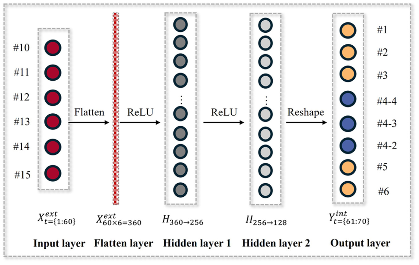
MLP architecture.

LSTM Model

The LSTM model implements a sequence-to-sequence architecture to effectively capture temporal dependencies in wind propagation through windbreak structures, as shown in Figure 3. The model employs an encoder–decoder framework where an encoder LSTM (hidden size = 64) processes a T-timestep sequence of exterior measurements, creating a compressed representation of the input time series. This representation is transferred to a decoder LSTM that generates predictions for interior wind conditions across S future timesteps. The mathematical formulation for each time step t in the input sequence is

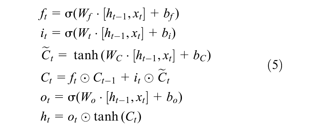
\begin{matrix} f_{t} = σ (W_{f} \cdot [h_{t - 1}, x_{t}] + b_{f}) \\ i_{t} = σ (W_{t} \cdot [h_{t - 1}, x_{t}] + b_{i}) \\ {\tilde{C}}_{t} = \tanh (W_{C} \cdot [h_{t - 1}, x_{t}] + b_{C}) \\ C_{t} = f_{t} ⊙ C_{t - 1} + i_{t} ⊙ {\tilde{C}}_{t} \\ o_{t} = σ (W_{o} \cdot [h_{t - 1}, x_{t}] + b_{o}) \\ h_{t} = o_{t} ⊙ \tanh (C_{t}) \end{matrix}

(5)

where f_t, i_t, and o_t are the forget, input, and output gates respectively, C_t is the cell state, h_t is the hidden state, and ⊙ represents element-wise multiplication. The final hidden state h_T and cell state C_T encapsulate the temporal patterns from the entire input sequence and are transferred to the decoder LSTM. The decoder then generates predictions sequentially according to

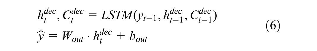
\begin{matrix} h_{t}^{dec}, C_{t}^{dec} = LSTM (y_{t - 1}, h_{t - 1}^{dec}, C_{t - 1}^{dec}) \\ \hat{y} = W_{out} \cdot h_{t}^{dec} + b_{out} \end{matrix}

(6)

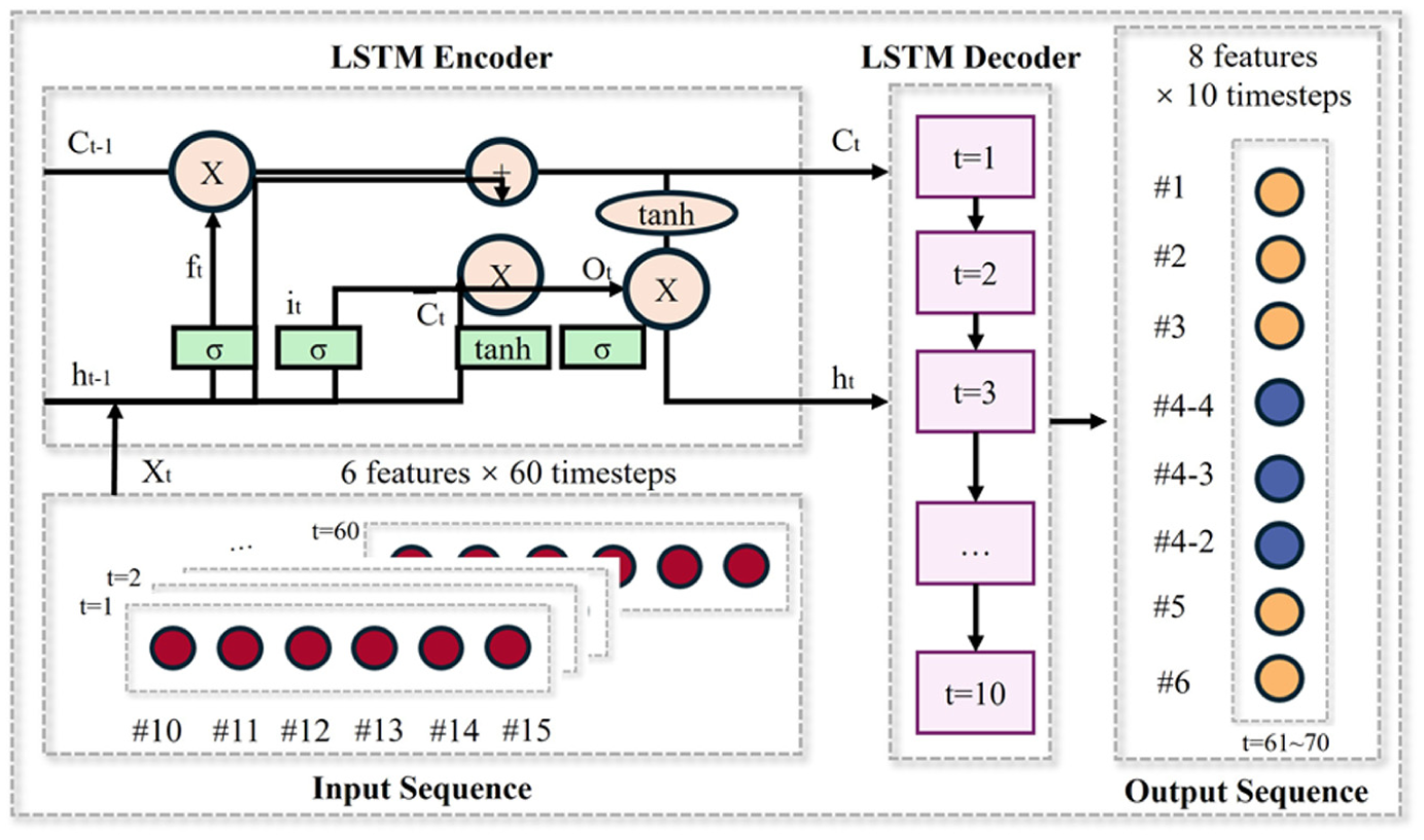
where the initial states are set as $h_{0}^{dec} = h_{T}$ and $C_{0}^{dec} = C_{T}$ from the encoder. During training, a teacher forcing mechanism is employed where ground truth values are occasionally substituted as decoder inputs to stabilize the learning process.

Figure 3.

LSTM architecture.

TCN Model

The TCN model employs dilated causal convolutions to effectively capture long-range dependencies while maintaining computational efficiency for wind field prediction. The architecture implements a hierarchical structure with three stacked temporal blocks, each featuring increasing dilation factors (1, 2, and 4), which exponentially expands the receptive field to encompass the entire historical sequence of T timesteps while using significantly fewer parameters than fully connected alternatives, as shown in Figure 4.

Figure 4.

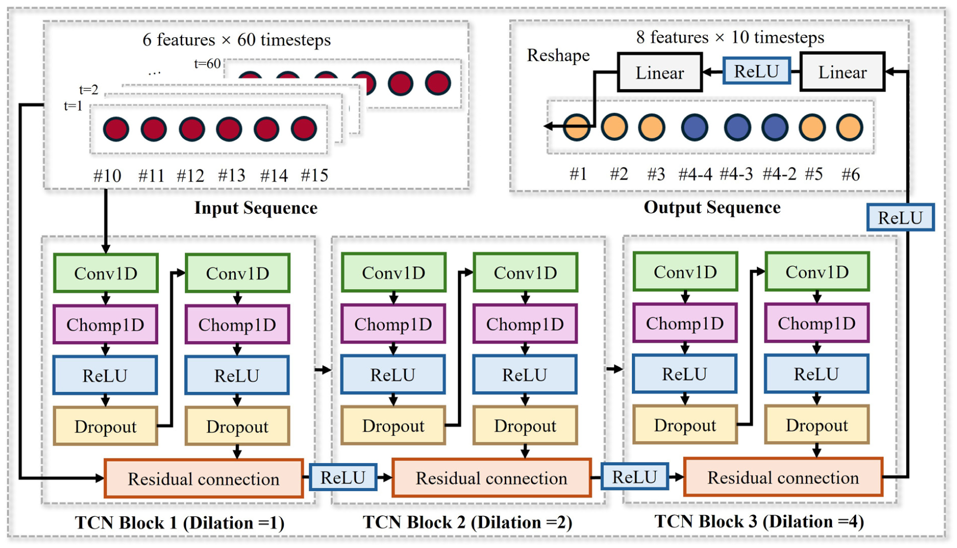
TCN architecture.

Mathematically, each dilated causal convolution layer applies the operation

F (s) = (x_{* d} f) (s) = \sum_{i = 0}^{k - 1} f (i) \cdot x_{s - d \cdot i}

(7)

where x is the input sequence, f is the filter of length k = 3, and d is the dilation factor that creates gaps between filter elements to capture broader temporal context. Each temporal block contains two weight-normalized convolutional layers with ReLU activations and dropout (rate = 0.2), connected by residual connections that facilitate gradient flow during training according to

o = Re LU (x + F (x))

(8)

where F(x) represents the convolution operations. The final output is processed through a two-layer projection network to generate multistep predictions. To strictly maintain the causal structure of the prediction, a custom layer named Chomp1d was incorporated after each convolution operation. Since standard convolution layers introduce symmetric padding, this module functions by truncating the padding on the right side of the sequence. This ensures that the model cannot access future information and that the output length remains consistent with the input across the temporal blocks.

N-BEATS Model

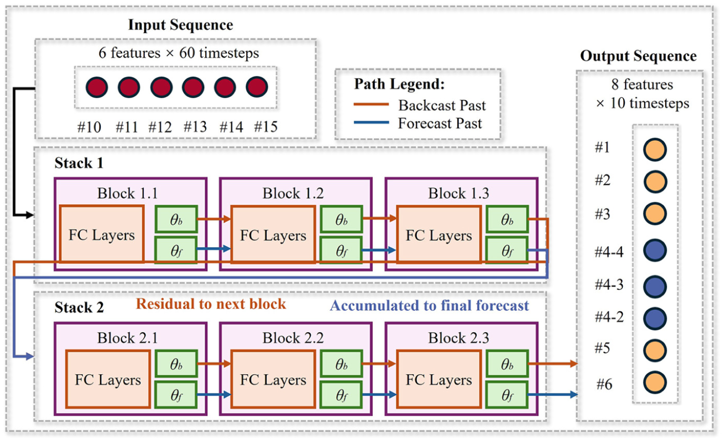
The N-BEATS model employs a hierarchical, basis-expansion architecture to tackle time series forecasting challenges. The model consists of multiple stacks of processing blocks arranged in a doubly residual configuration to enable effective learning at different temporal resolutions, as shown in Figure 5. Each block operates through a four-layer fully connected network that processes the input and projects the output onto learned basis functions through two separate pathways: the backward path (backcast) which reconstructs the input signal, and the forward path (forecast) which predicts future values. Mathematically, for an input sequence $x \in R^{T \times d}$ , where T is the sequence length and d is the dimensionality, each block performs:

\begin{matrix} θ_{b}, θ_{f} = F C_{stack} (x) \\ \hat{x} = G_{b} (θ_{b}) \\ \hat{y} = G_{f} (θ_{f}) \end{matrix}

(9)

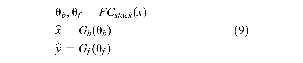
where θ_b and θ_f are the backcast and forecast basis coefficients, and G _b and G _f are the backward and forward basis functions. The architecture facilitates hierarchical decomposition of the time series into different interpretable components, allowing the model to capture both short-term patterns and long-term trends in the wind propagation data.

Figure 5.

N-BEATS architecture.

Transformer Model

The transformer architecture, initially proposed for natural language processing tasks, has emerged as a powerful paradigm for sequential data modeling across diverse domains ( 20 ). Unlike recurrent neural networks that process sequence elements sequentially, transformer employs a self-attention mechanism that enables parallel computation and captures long-range dependencies more effectively. The transformer architecture is shown in Figure 6. In the context of wind speed prediction, this architecture offers distinct advantages for modeling the complex temporal relationships between external and internal wind conditions around HSR barriers.

Figure 6.

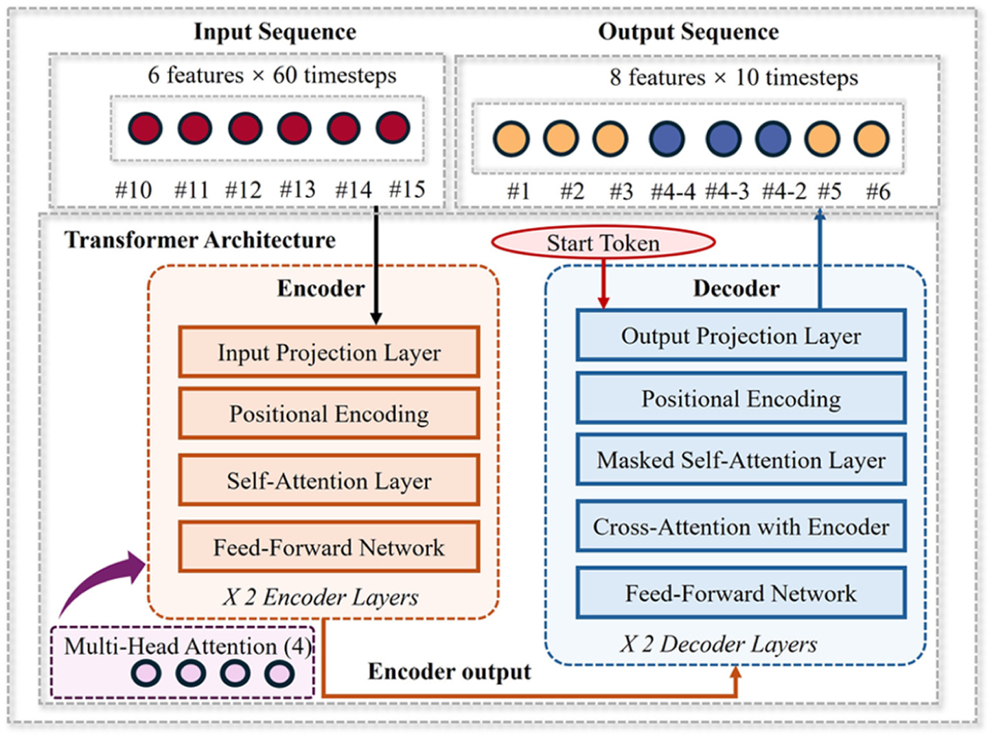
Transformer architecture.

The core component of the transformer is the self-attention mechanism, which computes the relevance between each pair of elements in the input sequence. For a given input sequence $X \in R^{n \times s}$ , where n is the sequence length and s is the feature dimension, the self-attention operation involves transforming the input into queries Q, keys K, and values V through learnable linear projections. The attention scores are then computed as

Attention (Q, K, V) = soft max (\frac{Q K^{T}}{\sqrt{d_{k}}}) V

(10)

where the scaling factor $\sqrt{d_{k}}$ prevents excessively large values in the dot products, particularly for large dimensions, which could push the SoftMax function into regions with extremely small gradients. To further enhance the model’s representational capacity, transformer employs multihead attention:

Multihead (Q, K, V) = Concat ({head}_{1}, \dots, {head}_{h})

(11)

where each head computes

{head}_{i} = Attention ({QW}_{i}^{Q}, {KW}_{i}^{K}, {VW}_{i}^{V})

(12)

Since the self-attention mechanism computes relationships in parallel without inherent sequence awareness, positional encodings are injected to provide the necessary temporal context. This ensures the model distinguishes between past and future states within the wind speed progression. We incorporate positional encoding to preserve temporal order information, as the self-attention mechanism itself is permutation-invariant:

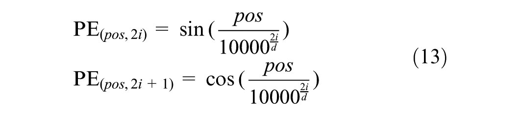
\begin{matrix} {PE}_{(pos, 2 i)} = \sin (\frac{pos}{10000^{\frac{2 i}{d}}}) \\ {PE}_{(pos, 2 i + 1)} = \cos (\frac{pos}{10000^{\frac{2 i}{d}}}) \end{matrix}

(13)

where pos is the position and i is the dimension. This encoding allows the model to leverage the relative positions of time steps in the wind speed sequences.

Model Configuration

To ensure the reproducibility of the experiments, all models were implemented using the PyTorch framework and trained on a high-performance workstation equipped with an NVIDIA RTX4070 GPU (CUDA 12.1) to accelerate computation. A fixed random seed of 42 was applied across NumPy, PyTorch, and Python random generators to guarantee deterministic initialization and data splitting. The hyperparameters for each model were determined through a grid search strategy during preliminary experiments, selecting the configurations that minimized the MSE on the training set. While the baseline models were trained for a fixed number of epochs to ensure full convergence, the transformer model utilized a dynamic training strategy involving a learning rate scheduler (ReduceLROnPlateau) and an early stopping mechanism. Specifically, the training of the transformer was halted if the test loss did not improve for 20 consecutive epochs to prevent overfitting. The specific hyperparameter settings and training configurations for all models are detailed in Table 1.

Table 1.

Model Configuration

Parameter	MLP	LSTM	TCN	N-BEATS	Transformer
Architecture	Feedforward neural network	Recurrent neural network	Temporal convolutional network	Deep residual network	Attention-based Seq2Seq
Hidden dimension	360→256→128	128	64→128→256	256	64 (d_model)
Layers/stacks	3 FC layers	2 LSTM layers	3 TCN blocks	2 stacks, 3 blocks	2 encoder, 2 decoder
Special parameters	Flattened: 360	NA	Kernel size: 3 Dilations: [1,2,4]	NA	Attention heads: 4
Dropout	0.2	0.2	0.2	NA	0.1
Activation function	ReLU	Tanh (internal)	ReLU	ReLU	ReLU
Learning rate	0.001	0.001	0.001	0.001	0.0005
Optimizer	Adam	Adam	Adam	Adam	Adam + reduce LR on plateau
Batch size	32	32	32	32	32
Epochs	1000	1000	1000	1000	1000 (with early stopping)
Gradient clipping	NA	NA	NA	1	1
Special training	NA	NA	NA	NA	Teacher forcing (0.5)
Time awareness	NA	Inherent sequence memory	Dilated convolutions	Hierarchical decomposition	Positional encoding
Parameters (approx.)	∼300K	∼200K	∼300K	∼500K	∼100K

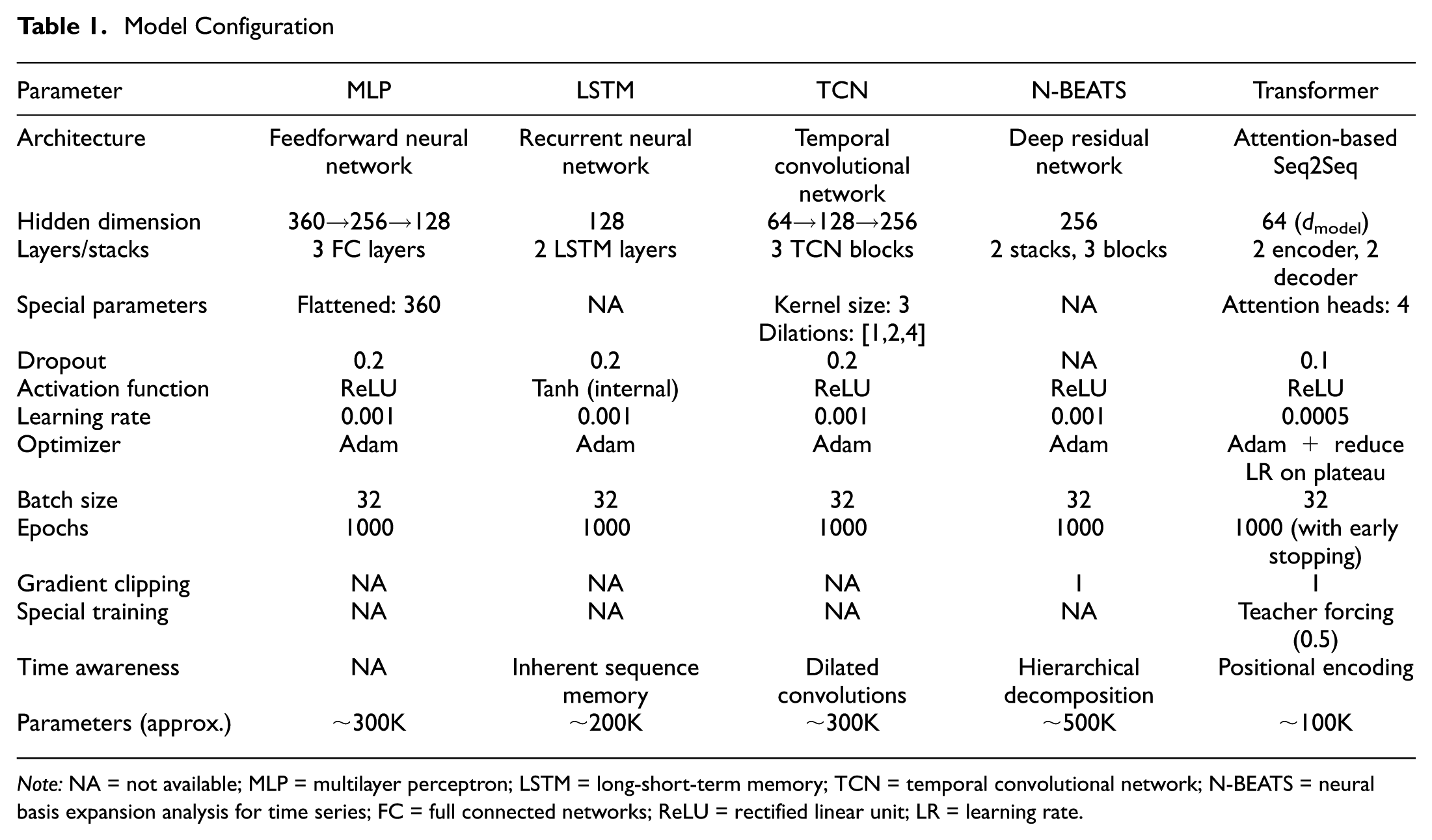
Note: NA = not available; MLP = multilayer perceptron; LSTM = long-short-term memory; TCN = temporal convolutional network; N-BEATS = neural basis expansion analysis for time series; FC = full connected networks; ReLU = rectified linear unit; LR = learning rate.

Results

Models Performance

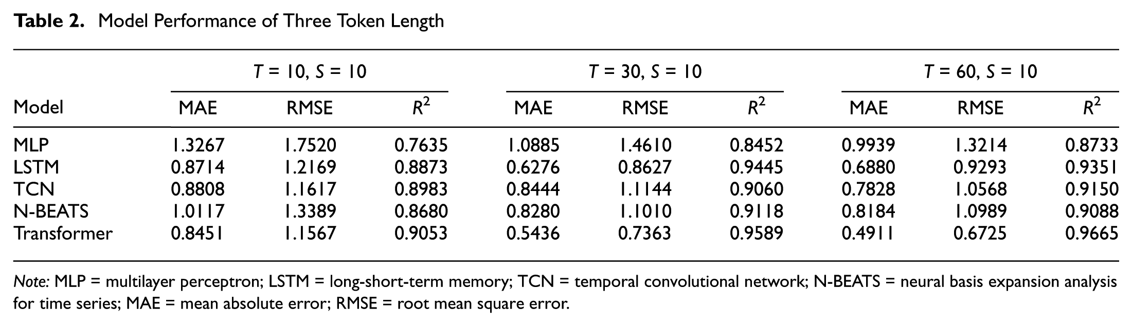
This section presents the models’ performance in the wind speed sequence prediction. Table 2 presents the comparative performance of five neural network models across three input token lengths (T = 10, 30, and 60) with a fixed prediction horizon of 10 steps (S = 10).

Table 2.

Model Performance of Three Token Length

Model	T = 10, S = 10			T = 30, S = 10			T = 60, S = 10
Model	MAE	RMSE	R ²	MAE	RMSE	R ²	MAE	RMSE	R ²
MLP	1.3267	1.7520	0.7635	1.0885	1.4610	0.8452	0.9939	1.3214	0.8733
LSTM	0.8714	1.2169	0.8873	0.6276	0.8627	0.9445	0.6880	0.9293	0.9351
TCN	0.8808	1.1617	0.8983	0.8444	1.1144	0.9060	0.7828	1.0568	0.9150
N-BEATS	1.0117	1.3389	0.8680	0.8280	1.1010	0.9118	0.8184	1.0989	0.9088
Transformer	0.8451	1.1567	0.9053	0.5436	0.7363	0.9589	0.4911	0.6725	0.9665

Note: MLP = multilayer perceptron; LSTM = long-short-term memory; TCN = temporal convolutional network; N-BEATS = neural basis expansion analysis for time series; MAE = mean absolute error; RMSE = root mean square error.

The results indicate that increasing the input token length generally improves forecasting accuracy across all models. As the historical sequence length increases from T = 10 to T = 60, both error metrics decrease while R² values rise. This trend suggests that providing models with longer historical context enables better capture of underlying temporal patterns in the data.

The transformer architecture demonstrates superior performance across all configuration scenarios, achieving the lowest error metrics and highest R² values. At T = 60, the transformer achieves remarkable performance with an MAE of 0.4911, RMSE of 0.6725, and R² of 0.9665. At this longest input length, the transformer’s MAE is approximately 29% lower than that of LSTM (0.6880) and 37% lower than that of TCN (0.7828), indicating that the performance gap between the transformer and the other competitive baselines becomes substantial as the historical context grows, even though the gap is smaller at T = 10. LSTM consistently performs as the second-best model, particularly excelling at T = 30 with an MAE of 0.6276 and R² of 0.9445. TCN and N-BEATS show competitive performance with different strengths across varying token lengths, while the MLP baseline, despite its simplicity, achieves reasonable but comparatively lower accuracy.

Figure 7 provides a visual representation of prediction performance through scatter plots of predicted versus true values for all models across different token lengths. The diagonal dashed line represents perfect prediction, with closer clustering around this line indicating better model performance. Each subplot displays both training (red) and test (blue) datasets with their respective R² values. The scatter plots reveal that the transformer model maintains the tightest clustering around the perfect prediction line, particularly at T = 60 where it achieves a test R² of 0.9665, demonstrating its superior generalization capability. It is noted that all models benefit from increased historical context, as scatter points progressively tighten around the diagonal line as token length increases from T = 10 to T = 60.

Figure 7.

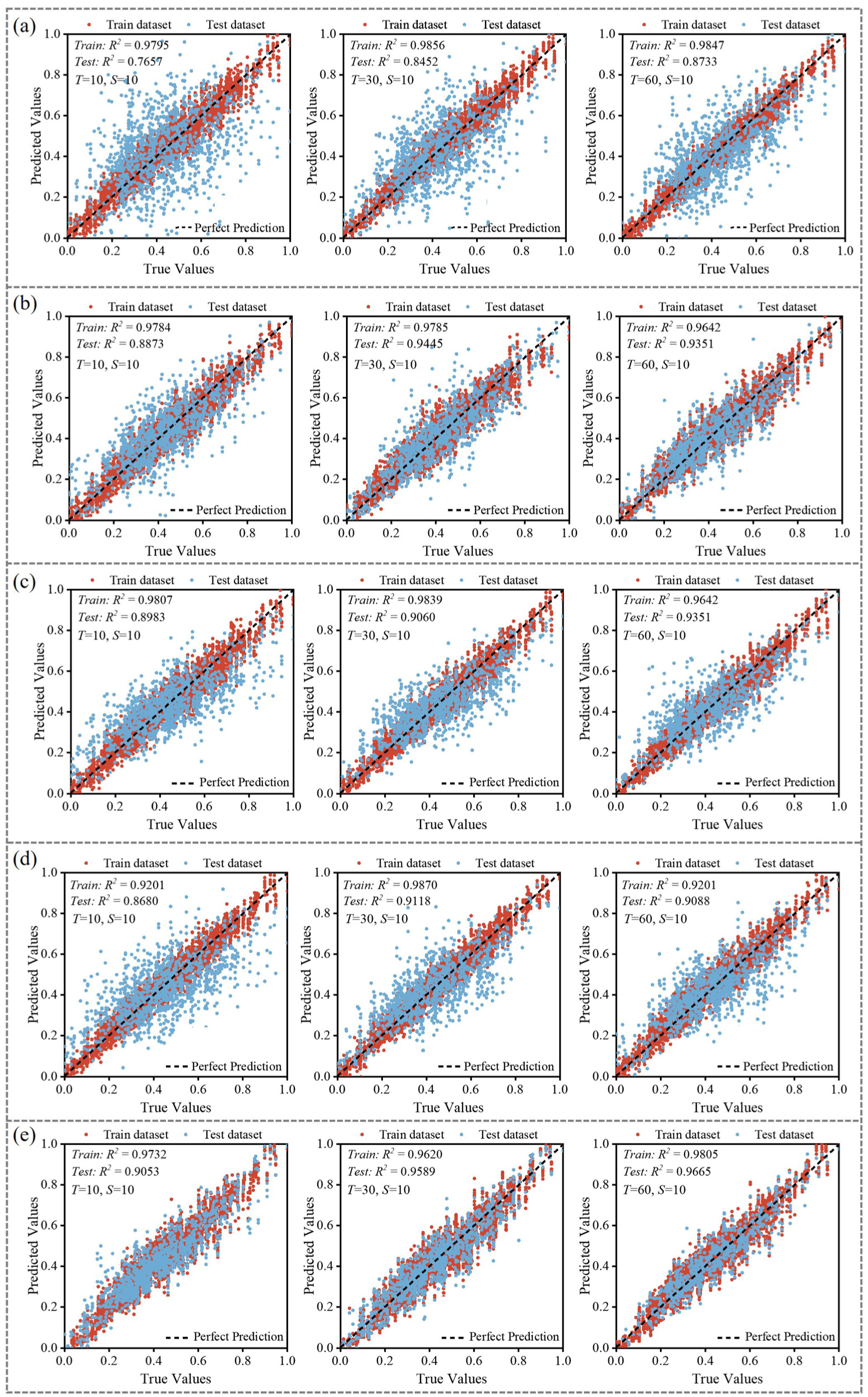
Model performance in different token length (T = 10, 30, 60) at Mast #1: (a) MLP, (b) LSTM, (c) TCN, (d) N-BEATS, and (e) transformer.

Notably, the gap between training and testing R² values provides insight into model generalization. The MLP shows the largest disparity, indicating potential overfitting, while the transformer maintains more consistent performance between training and testing sets. For T = 60, LSTM and TCN demonstrate nearly identical test R² values (0.9351), yet their scatter distributions show subtle differences in how they handle various ranges of the target variable. The most substantial performance improvements occur when increasing from T = 10 to T = 30, suggesting that a moderate historical context provides significant information gain. The relative performance gains when moving from T = 30 to T = 60 is less pronounced for most models except the transformer, which continues to show substantial improvement with longer sequences, highlighting the effectiveness of attention mechanisms in leveraging extended temporal context.

Token Length Analysis

Figure 8 illustrates the temporal prediction performance of all models against ground truth wind speed measurements across 100 consecutive time steps for three different input token lengths, taking Mast #1 as example. The time-series visualization provides additional insights beyond the aggregate metrics presented in Table 2. At T = 10 (Figure 8a), all models capture the general trend of wind speed fluctuations, but significant notable discrepancies occur at extreme values. The MLP model exhibits the largest deviations, particularly at wind speed peaks and troughs, confirming its higher error metrics. The transformer and LSTM demonstrate better tracking of the ground truth pattern, though all models struggle with sharp transitions in wind speed. With increased token length to T = 30 (Figure 8b), prediction accuracy improves across all models. The transformer and LSTM more precisely track the ground truth trajectory, with reduced phase shifts and amplitude errors. The N-BEATS model shows improvement in capturing the temporal dynamics compared with its T = 10 performance. However, some discrepancies remain during rapid wind speed changes, suggesting challenges in predicting sudden meteorological shifts. At T = 60 (Figure 8c), the most substantial improvements are observed in the transformer model, which closely follows the ground truth trajectory throughout the sequence with minimal deviations. The LSTM model maintains strong performance, while TCN and N-BEATS show moderate improvements over their T = 30 counterparts. The MLP continues to exhibit larger oscillations around the actual values, particularly at peaks, though its overall tracking has improved from shorter token lengths.

Figure 8.

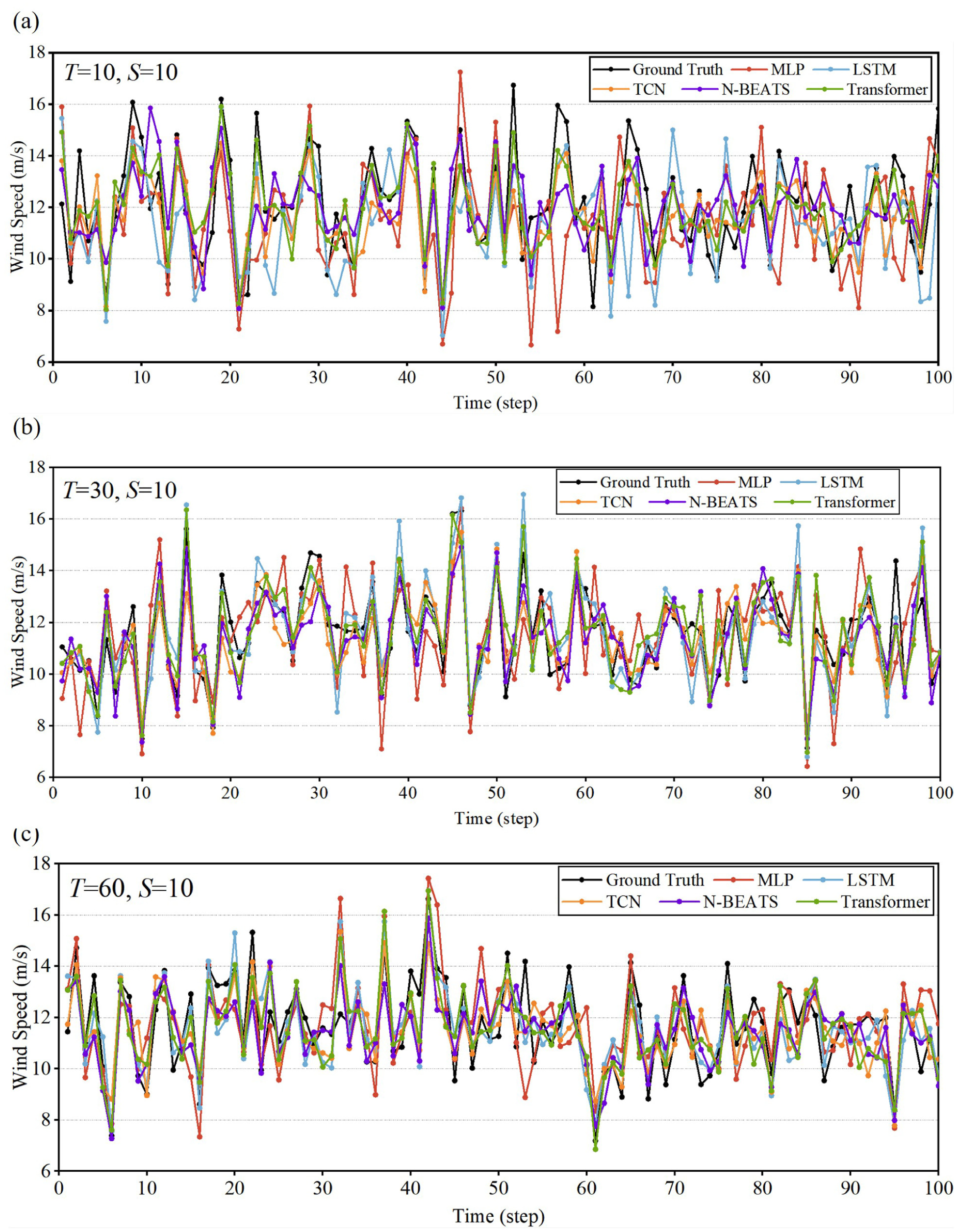
Prediction output in different token length at Mast #1: (a) T = 10, (b) T = 30, and (c) T = 60.

Across all token lengths, a common observation is that prediction errors tend to occur predominantly at transition points where wind speed changes rapidly, while periods of relative stability are predicted with higher accuracy by all models. The visualization confirms the quantitative findings that longer historical contexts enable more accurate predictions, with the transformer architecture most effectively leveraging extended temporal information to produce precise forecasts.

Mast Predictability

Figure 9 presents the time-series comparison between transformer model predictions (T = 60, S = 10) and ground truth wind speeds across different anemometer mast locations. These visualizations illustrate the varying performance of the transformer model across spatial locations over a 50-time step horizon, demonstrating how the optimal configuration performs in practice at each measurement site.

Figure 9.

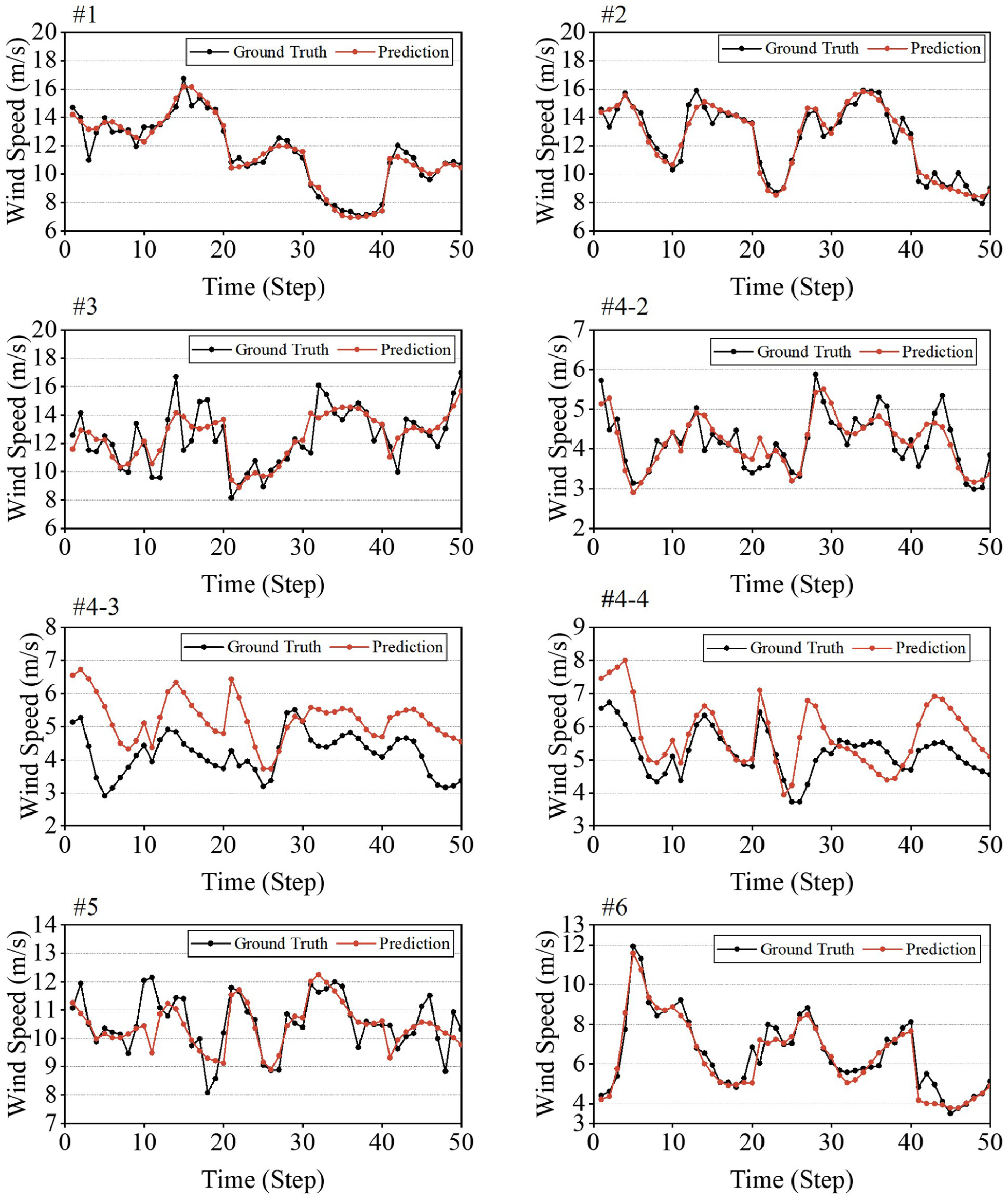
Anemometer mast prediction results.

Masts #1, #2, and #6 demonstrate the highest prediction accuracy, with forecasted values closely tracking the ground truth trajectories throughout most time steps. The close alignment between the prediction and ground truth lines indicates that the model effectively captures both the magnitude and the phase of wind speed fluctuations. This superior predictability offers a post hoc physical insight into the flow field. Specifically, Masts #1 and #2 are situated further downstream where the chaotic wake turbulence generated by the windbreak wall has likely restabilized into a coherent flow pattern, significantly reducing stochastic noise. Similarly, Mast #6 appears to benefit from its direct spatial alignment with the high-importance exterior measurement points, creating a strong linear correlation that the transformer architecture effectively captures.

In contrast, Masts #4-3 and #4-4 show notable discrepancies between transformer predictions and actual measurements, with consistent overestimation of wind speeds across most time steps. This systematic bias can be attributed to the height differences between measurement locations—while most anemometer masts are positioned at a height of approximately 2m, Masts #4-3 and #4-4 are installed at heights of 3m and 4m, respectively. The model fails to adequately account for these elevation differences and their impact on vertical wind profiles, where wind speed typically increases with height because of reduced surface friction. As a result, the model struggles to generalize patterns learned primarily from standard-height masts to these higher-positioned sensors. Mast #3 presents an interesting case where predictions accurately follow moderate wind speeds but struggle to capture extreme peaks, as evident around time steps 15–20 and 50, where sharp increases in wind speed are underestimated by the model. Similarly, Mast #5 shows generally good tracking of the temporal pattern but misses certain localized peaks and troughs in the wind speed signal.

Figure 10 presents a comparative analysis of model performance across different anemometer masts with the optimal configuration of T = 60 and S = 10. The normalized R² values for both training and testing datasets provide insights into location-specific predictability and model generalization capabilities.

Figure 10.

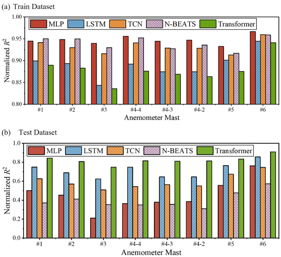
Mast predictability (T = 60, S = 10): (a) train dataset, and (b) test dataset.

In the training dataset (Figure 10a), all models achieve relatively high performance with normalized R² values consistently above 0.80. The MLP and N-BEATS models demonstrate particularly strong fitting capabilities on the training data, with MLP achieving the highest R² values at Masts #4-4 and #6. The transformer, while showing good performance, exhibits slightly lower training R² values compared with other models at most mast locations, except for Mast #6 where all models perform exceptionally well. The test dataset results (Figure 10b) reveal substantial differences in model generalization across locations. The transformer consistently outperforms other models across nearly all masts, maintaining normalized R² values around 0.80, which indicates robust generalization capability. LSTM shows the second-best performance in testing, particularly excelling at Mast #6 where it achieves the highest R² value among all models. In contrast, MLP and N-BEATS exhibit the largest performance degradation between training and testing datasets, suggesting potential overfitting to the training data.

Notable variations in predictability exist between different anemometer masts. Mast #6 demonstrates the highest predictability across all models for both training and testing datasets, suggesting that the wind patterns at this location may have more regular and learnable characteristics. Conversely, Masts #3 and #4-4 show lower predictability, particularly in the test dataset, indicating more complex or stochastic wind behavior that presents greater forecasting challenges. The gap between training and testing performance varies significantly by location. For instance, at Mast #4-3, all models show a substantial performance drop in testing compared with training, suggesting location-specific challenges in generalizing learned patterns. This spatial variability in predictability highlights the importance of considering location-specific factors in wind speed forecasting applications and the need for models that can generalize effectively across diverse geographical conditions. The consistent performance of the transformer across different mast locations underscores its robust generalization capability, likely because of its attention mechanism effectively capturing both short and long-range dependencies in the temporal data regardless of location-specific variations. This finding suggests that attention-based architecture may offer advantages for wind forecasting applications that require consistent performance across multiple measurement locations.

Feature Importance Analysis

Figures 11 and 12 provide insights into the feature importance dynamics across different masts and their temporal characteristics, offering valuable understanding of the underlying predictive mechanisms in wind speed forecasting.

Figure 11.

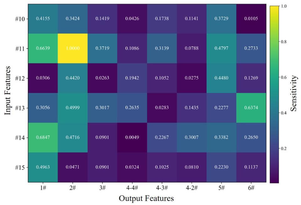
Input–output sensitivity analysis.

Figure 12.

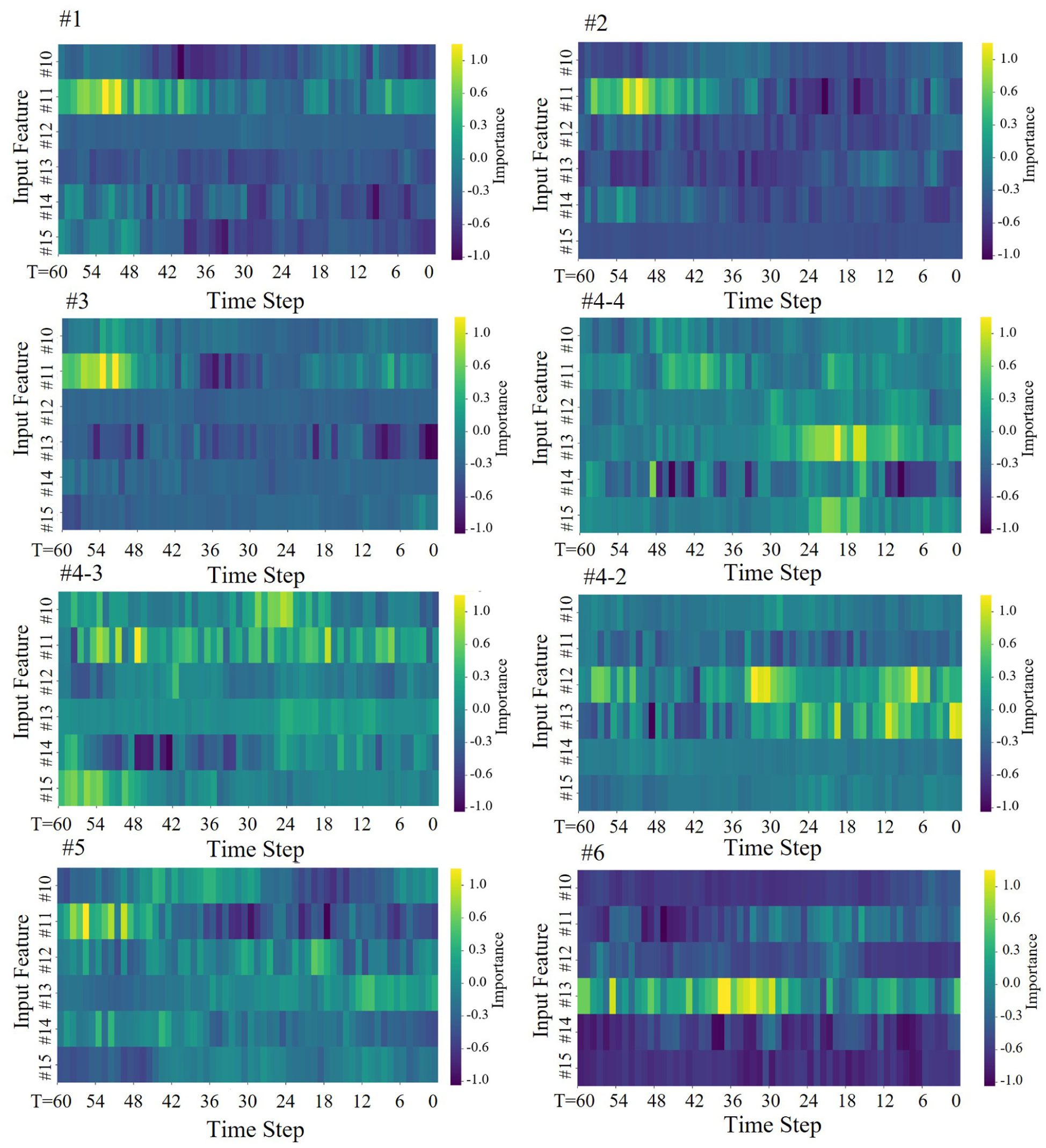
Temporal feature importance (normalized).

Figure 11 presents a heatmap of normalized input–output sensitivity analysis, revealing the relative influence of different mast inputs (#10 to #15) on the prediction of target masts (#1 to #6). The results demonstrate significant heterogeneity in cross-mast relationships. Input from Mast #11 exhibits exceptionally high sensitivity to output #2 (1.0000), indicating a dominant predictive relationship. Similarly, strong sensitivities are observed between inputs #14 and #11 to output #1 (0.6847 and 0.6639, respectively), suggesting that these locations provide critical information for forecasting at Mast #1. Notably, Mast #13 shows substantial influence on Mast #6 (0.6374), while having minimal impact on Mast #4-3 (0.0283). This highlights the spatial dependency structure of wind patterns across the measurement network. The lowest sensitivities are observed between input #12 and output #1 (0.0306), and input #14 and output #4-4 (0.0049), indicating near independence between these measurement locations. Overall, the sensitivity matrix reveals that geographic proximity alone does not determine predictive relationships, as some physically distant masts demonstrate stronger correlations than adjacent ones, likely because of complex terrain effects and wind patterns in the region.

Figure 12 extends our analysis by visualizing the temporal dynamics of feature importance across different output locations. The normalized temporal importance profiles reveal distinct patterns unique to each target mast. For Masts #1 and #2, input features #10 and #11 demonstrate consistently high importance, particularly at time steps 42–54. Mast #3 shows strong positive importance for feature #11 at earlier time steps (48–54), while Mast #4-4 displays a striking pattern with feature #15 showing high positive importance in recent time steps (0–12) and feature #14 exhibiting strong negative importance at multiple intervals. Mast #4-3 features notable importance from both features #11 and #15, while Mast #4-2 shows distinctive patterns for features #12 and #15. For Mast #5, features #10 and #11 consistently demonstrate high importance across early time steps, while Mast #6 shows particularly strong importance for feature #13 across extended periods (24–42).

The negative importance values (dark purple regions [color online only]) indicate inverse relationships between certain inputs and outputs at specific time steps, which is particularly evident in Masts #4-4, #4-2, and #6. These inverse relationships can be as valuable for prediction as positive ones, providing counterbalancing signals in the forecasting models. The heterogeneous and complex nature of these relationships explains why sophisticated models such as transformers, with their ability to capture long-range dependencies and selectively attend to relevant features, outperform simpler architectures in this forecasting task.

Figure 13 further extends our feature importance analysis, providing both detailed rankings and consolidated importance scores across all prediction targets. As shown in Figure 13a, input feature #11 consistently demonstrates the highest importance ranking across all output locations. This dominant pattern aligns with the high sensitivity observed in Figure 11, particularly for output #2. Similarly, input feature #10 consistently ranks as the second most important feature across most targets, with normalized importance scores ranging from 0.67 to 0.98, reinforcing its strong influence observed in the sensitivity analysis.

Figure 13.

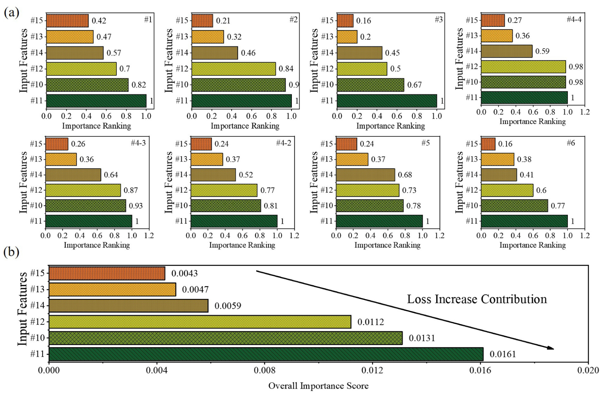
Input features importance: (a) importance ranking of input features, and (b) overall importance score.

The hierarchical importance pattern remains remarkably consistent across all prediction targets, with features #11, #10, and #12 forming the top tier, while features #14, #13, and #15 consistently show lower importance values. This consistency suggests an underlying structure in the wind dynamics that transcends individual measurement locations. Interestingly, input #15 maintains its position as the least important feature across most targets. The normalization approach used in ranking facilitates clear comparison across different output targets, highlighting the relative contribution of each input feature regardless of the absolute magnitude of its effect. Figure 13b quantifies these relationships through loss increase contribution to measure how prediction error increases when each feature is removed or perturbed. This consolidated view confirms Mast #11’s critical role with the highest overall importance score (0.0161), followed by Mast #10 (0.0131), #12 (0.0112), #14 (0.0059), #13 (0.0047), and #15 (0.0043). These absolute values provide insight into the magnitude of each feature’s contribution to prediction accuracy.

The spatial distribution analysis reveals that feature importance does not strictly adhere to proximity relationships, indicating that topographical features and regional wind patterns create complex interdependencies beyond simple distance correlations. The dominance of Mast #11 in the importance hierarchy suggests a direct aerodynamic correlation with the flow structures driving the internal wind field. Physically, this implies that Mast #11 is likely positioned within the primary upstream wind corridor where the incoming flow exhibits the highest coherence and is least perturbed by local terrain roughness, thereby serving as a robust proxy for the free-stream velocity acting on the windbreak structure. Conversely, the consistently low importance of Mast #15 suggests it may be situated in a region of local aerodynamic separation or topographic shielding where measurements are dominated by localized turbulence or wake effects physically decoupled from the main flow propagation. This distinction demonstrates that the transformer model has effectively learned to filter out unrepresentative measurement points that do not reflect global flow dynamics, prioritizing inputs that preserve the physical continuity of the wind field. These insights offer a reference for optimizing sensor deployment, suggesting that strategic placement based on aerodynamic importance yields superior forecasting utility compared with uniform distribution.

Missing Input Features Influence

In operational wind forecasting systems, missing data are an inevitable challenge because of sensor malfunctions, communication failures, or maintenance activities. The resilience of forecasting models to missing input features is therefore critical for maintaining prediction reliability in real-world applications. Different strategies for handling missing data can significantly affect model performance, with some approaches potentially preserving forecasting capabilities even under substantial data loss conditions.

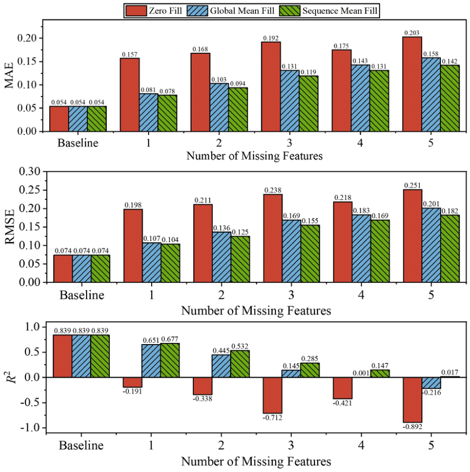
Figure 14 presents a comprehensive analysis of three common missing data handling strategies, including zero filling, global mean filling, and sequence mean filling, and their impact on model performance as measured by MAE, RMSE, and R² metrics. Table 3 provides detailed R² values for each strategy across different scenarios of missing input features.

Figure 14.

Comparison of different filling strategies.

Table 3.

Comparison of Different Filling Strategies (R²)

Filling strategy	Baseline	1 Missing	2 Missing	3 Missing	4 Missing	5 Missing
Zero filling	0.839	−0.191	−0.338	−0.712	−0.421	−0.892
Global mean filling	0.839	0.651	0.445	0.145	0.001	−0.216
Sequence mean filling	0.839	0.677	0.532	0.285	0.147	0.017

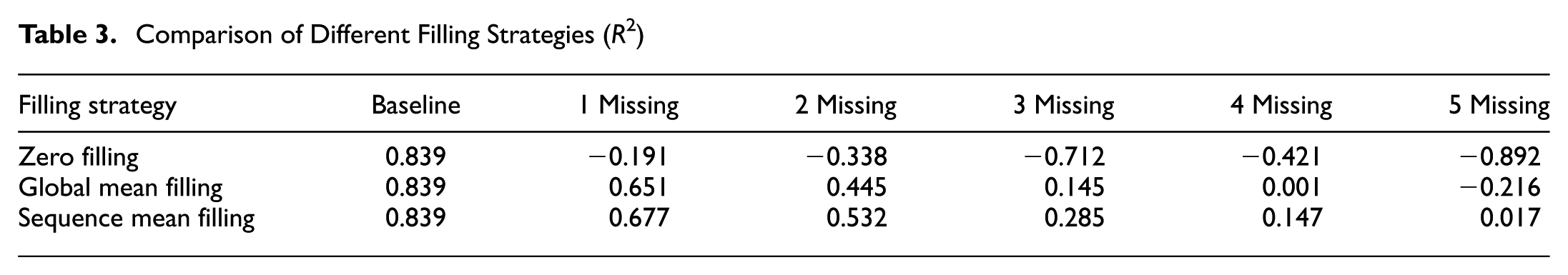
The baseline scenario, where all input features are available, establishes identical performance across all three strategies with an R² of 0.839, indicating strong predictive capability under optimal data conditions. However, as the number of missing features increases, significant performance divergence emerges between the different filling strategies.

Zero filling, which replaces missing values with zeros, demonstrates the poorest resilience to missing data. The R² values rapidly deteriorate into negative territory, reaching −0.191 with just one missing feature and plummeting to −0.892 with five missing features. This indicates that zero filling not only fails to maintain predictive power but also actively introduces harmful bias that makes predictions worse than a simple mean-based forecast. The MAE and RMSE metrics for zero filling show corresponding degradation, increasing from baseline values of 0.054 and 0.074 to 0.203 and 0.251, respectively, with five missing features.

Global mean filling, which replaces missing values with the average of all available data points for that feature, demonstrates substantially better resilience. With one missing feature, it maintains a respectable R² of 0.651, and performance degrades more gradually as missing features increase. However, its effectiveness diminishes considerably with four or more missing features, where R² approaches zero (0.001) and eventually becomes negative (−0.216) with five missing features.

Sequence mean filling performs best among the three strategies tested, replacing missing values with the mean of the available values within the same sequence. This strategy consistently outperforms the alternatives across all scenarios, maintaining positive R² values even with five missing features (0.017). The performance degradation is more gradual, with R² values of 0.677, 0.532, 0.285, and 0.147 for one to four missing features, respectively. The MAE and RMSE metrics for sequence mean filling also show the slowest rate of increase among the three strategies.

The superior performance of sequence mean filling can be attributed to its ability to preserve temporal patterns within each data sequence, thereby maintaining the contextual integrity of the input features. This approach leverages the temporal correlation structure within each feature sequence, which appears more informative than using global statistics that ignore temporal dependencies. Global mean filling, while better than zero filling, fails to capture these temporal dynamics, resulting in its intermediate performance. These findings have important implications for operational wind forecasting systems. The results demonstrate that appropriate missing data handling strategies can significantly mitigate performance degradation, with sequence-based approaches offering the most resilience. Implementation of sequence mean filling should be prioritized in operational forecasting systems to ensure prediction reliability during inevitable periods of partial data availability. Furthermore, the substantial performance differences between these simple strategies suggest that more sophisticated imputation methods, such as those based on temporal interpolation or machine learning approaches, might yield even greater robustness to missing data.

Discussion

The superior performance of transformer models for wind field prediction around railway infrastructure demonstrates the efficacy of attention mechanisms in capturing complex temporal dependencies in wind data. While achieving remarkable accuracy (R² = 0.9665), the analysis reveals that prediction performance varies substantially across measurement locations, suggesting fundamental aerodynamic differences in wind behavior around windbreak structures ( 31 ). The spatial heterogeneity in predictability challenges the development of universally applicable models and highlights the importance of location-adaptive approaches ( 32 , 33 ). Our feature importance analysis reveals complex interdependencies between measurement points that transcend simple geographic proximity, with certain exterior masts exhibiting disproportionate influence on specific interior locations. This pattern suggests underlying flow structures and channeling effects that could inform both sensor placement strategies and windbreak design optimization. The resilience analysis further demonstrates that appropriate missing data handling strategies, particularly sequence mean filling, can maintain positive predictive power even with substantial sensor loss, which has direct implications for cost-effective monitoring network design in both transportation and energy applications.

The successful application of the transformer architecture in this context relies on the specific physical characteristics of atmospheric turbulence, which naturally circumvent common computational bottlenecks. Unlike natural language processing tasks where semantic dependencies can span thousands of tokens, the effective correlation time of turbulent wind fluctuations is physically bounded because of chaotic decay. This property allows the model to capture all necessary dynamic information within concise context windows (e.g., 60 steps), thereby avoiding the memory and computational costs associated with processing extremely long sequences. Simultaneously, to address the risk of overfitting inherent to shorter field experiments, the sliding window strategy generates a dense dataset of overlapping samples, ensuring robust convergence within this effective temporal range.

In relation to the dataset duration, while the 4-h window focuses on a specific strong wind event, this selection targets the safety-critical scenarios that pose the highest risk to railway operations, prioritizing extreme dynamics over long-term calm conditions (34 –36). To address the challenge of cross-climate and seasonal generalizability, we propose the adoption of a transfer learning framework in future works ( 37 , 38 ). Under this scheme, the transformer model pretrained on this high-resolution dataset would serve as a backbone, requiring only limited fine-tuning data from new locations to adapt to local terrain or seasonal air density variations. This strategy effectively mitigates the single-site limitation by transforming the current site-specific solution into a scalable network-wide forecasting system. In addition, the fixed sampling frequency of 1 Hz represents a necessary compromise between resolution and computational feasibility, though multiresolution approaches could be explored to better capture high-frequency turbulence (39 –41). Finally, future iterations should move beyond treating wind speed and direction as separate targets by adopting integrated vector-based architectures, which would better represent the physical coupling inherent in fluid dynamics ( 42 ).

The predictive performance and robustness of the transformer model offer tangible benefits for HSR operational policy and infrastructure management. Economically, the varying feature importance levels suggest that a uniform sensor redundancy strategy is unnecessary. Instead, a targeted maintenance approach that prioritizes critical nodes such as Masts #10 and #11, while streamlining hardware at peripheral locations such as Masts #13 and #15, could potentially reduce hardware redundancy and associated maintenance costs, although the actual savings would depend on site-specific deployment conditions and are not quantified in this study. From a safety perspective, the model’s MAE of 0.49 m/s at T = 60 is well below the wind-speed thresholds typically used to trigger HSR speed restrictions (on the order of several m/s) ( 43 , 44 ). This precision suggests the proposed method could potentially serve as a virtual sensing approach for the train control system during hardware outages ( 45 ). Furthermore, the study supports a tiered protocol for sensor failures where data loss at low-impact masts can be mitigated via sequence mean filling without disrupting schedules, whereas failures at critical nodes such as Mast #11 may warrant additional caution, such as conservative speed restrictions, until the sensor is restored.

Furthermore, while the transformer architecture demonstrates superior predictive accuracy, we acknowledge that it operates primarily as a data-driven engine without explicit knowledge of fluid dynamics. The model minimizes statistical error rather than satisfying physical laws, which allows for potential violations of mass or momentum conservation in its predictions ( 46 ). To address this limitation, future iterations of this work should explore physics-informed neural networks ( 47 ). By incorporating residuals from the Navier–Stokes equations directly into the loss function, the model can be constrained to generate predictions that are not only statistically accurate but also physically consistent ( 48 , 49 ). Such an approach would significantly enhance the interpretability of the model, ensuring that the predicted wind fields adhere to the fundamental principles of flow continuity and energy conservation, thereby increasing engineering confidence for deployment in safety-critical railway systems ( 50 ).

Future research should extend this analysis to longer time periods capturing seasonal variations and extreme weather events to enhance model robustness. Incorporating physics-informed constraints into neural network architectures represents a promising direction that could improve both interpretability and generalization while potentially reducing data requirements through physical-informed regularization ( 51 ) and reinforcement learning ( 52 ). Developing multiresolution approaches that analyze different frequency bands separately could potentially reveal additional predictive patterns, especially for turbulent flow conditions around complex infrastructure. The observed spatial variability in predictability suggests potential benefits from transfer learning approaches, where models pretrained on data-rich locations could be fine-tuned for locations with limited historical data. Future work should also explore joint vector prediction models that simultaneously forecast wind speed and direction, better representing their inherent coupling (53 –55). From an implementation perspective, optimizing model architectures for edge computing deployment would address the computational challenges identified in this study, enabling real-time prediction capabilities for operational railway systems. These advancements would further bridge the gap between theoretical modeling capabilities and practical applications in both transportation safety and renewable energy domains.

Conclusion

This study investigated the application of various deep learning models, particularly the transformer architecture, for wind field prediction around HSR windbreak structures. Through comprehensive evaluation and comparison, we demonstrated that transformer-based models offer superior performance for this task, with significant implications for both transportation safety and renewable energy applications. The main conclusions from this study are:

The transformer model achieved the best overall performance among the five evaluated architectures (MLP, LSTM, TCN, N-BEATS, and transformer), achieving remarkable accuracy with an R² of 0.9665, MAE of 0.4911, and RMSE of 0.6725 when utilizing a 60-timestep historical context.

Prediction accuracy improved substantially as historical context increased from 10 to 60 timesteps, with the transformer exhibiting the most significant gains. This demonstrates the importance of sufficient temporal context for accurate wind field forecasting.

Considerable predictability variation was observed across measurement locations, suggesting that site-specific factors should be taken into account when deploying such models in different railway environments.

Feature importance analysis revealed complex spatial interdependencies between measurement points, with a consistent importance hierarchy emerging across all prediction targets. Masts #11 and #10 demonstrated high predictive correlation (with normalized importance scores frequently reaching 1.0 and over 0.8, respectively), while others (#15, #13) showed consistently lower importance. This clear ranking suggests more efficient resource allocation through prioritized maintenance of high-impact sensors and strategic placement of measurement equipment in future installations, potentially reducing infrastructure costs while maintaining forecasting accuracy.

Among the three missing-data handling strategies tested, sequence mean filling performed best, retaining positive predictive power up to four missing features and approaching zero only at five missing features (R² = 0.017), which is more robust than zero filling and global mean filling under the same conditions.

The methodologies developed in this study provide a foundation for next generation forecasting systems that can better manage the challenges at the intersection of transportation infrastructure, renewable energy development, and environmental variability.

Footnotes

Acknowledgements

The authors reviewed all content and take full responsibility for the accuracy and integrity of the work.

Authors’ Note

The authors utilized ChatGPT-4.0 exclusively for improving the language quality of this manuscript.

Author Contributions

The authors confirm contribution to the paper as follows: study conception and design: Jia-Hao Lu and Yuan-Jiang Zeng; data collection: Zheng-Wei Chen, Xiao-Tong-De Wang, and Yue-Yi Xiao; analysis and interpretation of results: Jia-Hao Lu; draft manuscript preparation: Jia-Hao Lu and Yuan-Jiang Zeng. All authors reviewed the results and approved the final version of the manuscript.

Declaration of Conflicting Interests

The authors declared no potential conflicts of interest with respect to the research, authorship, and/or publication of this article.

Funding

The authors disclosed receipt of the following financial support for the research, authorship, and/or publication of this article: This work was supported by the National Natural Science Foundation of China (Grant No. 52202426), and grants from the Research Grants Council of the Hong Kong Special Administrative Region, China (Grant Nos. 15205723 and 15226424).

ORCID iD

Jia-Hao Lu

Data Accessibility Statement

Data is available on reasonable request.

References

Jung

Recent Development and Future Perspective of Wind Power Generation. Energies, Vol. 17, 2024, p. 5391.

McKenna

Lilliestam

Heinrichs

H. U.

Weinand

Schmidt

Staffell

Hahmann

A. N.

, P. et al. System Impacts of Wind Energy Developments: Key Research Challenges and Opportunities. Joule, Vol. 9, 2025, p. 101799.

Khan

Al-Ammar

E. A.

Naeem

M. R.

Choi

H.-J.

Kang

H.-K.

Forecasting Renewable Energy for Environmental Resilience through Computational Intelligence. PLoS ONE, Vol. 16, 2021, p. e0256381.

Wang

Zhang

Yan

Han

Liu

A Comprehensive Review for Wind, Solar, and Electrical Load Forecasting Methods. Global Energy Interconnection, Vol. 5, 2022, pp. 9–30.

Chen

Zhang

Xiong

Cheng

Analysis of Wind Speed Characteristics along the High-Speed Railway. Applied Sciences, Vol. 15, 2024, p. 138.

Chen

Z.-W.

Guo

Z.-H.

Y.-Q.

Liu

T.-H.

Zhang

A Suction Method to Mitigate Pressure Waves Induced by High-Speed Maglev Trains Passing Through Tunnels. Sustainable Cities and Society, Vol. 96, 2023, p. 104682.

Chen

Z.-W.

Zeng

G.-Z.

Y.-Q.

Liu

T.-H.

Niu

J.-Q.

Yao

H.-D.

Reducing the Aerodynamic Drag of High-Speed Trains by Air Blowing From the Nose Part: Effect of Blowing Speed. Journal of Wind Engineering and Industrial Aerodynamics, Vol. 238, 2023, p. 105429.

Huo

Liu

Chen

Wang

Prediction of Train Aerodynamic Coefficients under Diverse Shape Parameters and Yaw Angles. Journal of Computational Design and Engineering, Vol. 12, 2025, pp. 184–203.

Mohebbi

The Influence of Inclined Barriers on Airflow Over a High Speed Train under Crosswind Condition. In New Research on Railway Engineering and Transportation ( Hessami

A. G.

Muttram

, eds.), IntechOpen, 2023, p. 112751.

10.

Deng

Yang

Zhu

Wang

Zhou

Aerodynamic Response of High-Speed Trains under Crosswind in A Bridge-Tunnel Section With or Without a Wind Barrier. Journal of Wind Engineering and Industrial Aerodynamics Vol. 210, 2021, pp. 104502.

11.

Guo

Z.-J.

Peng

Guo

Z.-H.

Zeng

Y.-J.

J.-H.

Chen

Z.-W.

Aerodynamic Performance and Operational Safety of High-Speed Trains in Crosswind: Visualization and Analysis of Mapping Knowledge Domain. Journal of Wind Engineering and Industrial Aerodynamics, Vol. 270, 2026, p. 106337.

12.

Xiong

Wang

Zhang

Pan

Liu

Tang

Liu

Sustainable Wind Barrier: Self-Powered System for High-Speed Railway Safety Monitoring. Sustainable Materials and Technologies, Vol. 39, 2024, p. e00848.

13.

Wang

Jiang

Lin

Yousif

Yuan

Zhou

Field Measurement on the Wind and Thermal Microenvironment of Distributed PV Array. Journal of Building Engineering, Vol. 105, 2025, p. 112492.

14.

Xing

Yang

Shi

Liu

Artificial-Intelligence-Based Model for Early Strong Wind Warnings for High-Speed Railway System. Electronics, Vol. 13, 2024, p. 4582.

15.

Madkour

F. E.

Lowry

Abdel-Rahim

Hammad

Vibhav

Paulo

Analysis of Wind Force on Cyclists From Passing Vehicles. Transportation Research Record, 2023. 2677: 340–352.

16.

Lim

Zohren

, Time-Series Forecasting With Deep Learning: A Survey. Philosophical Transactions of the Royal Society A: Mathematical, Physical and Engineering Sciences, Vol. 379, 2021, p. 20200209.

17.

Torres

J. F.

Hadjout

Sebaa

Martínez-Álvarez

Troncoso

Deep Learning for Time Series Forecasting: A Survey. Big Data, Vol. 9, 2021, pp. 3–21.

18.

Xie

Zhang

Shi

Intelligent Long-Term Prediction of Wind-Induced Response of Super High-Rise Buildings during Typhoons Based on Wind Tunnel Tests. Journal of Building Engineering, Vol. 103, 2025, p. 112144.

19.

Chen

Lin

Xie

Real-Time Yaw-Misalignment Calibration and Field-Test Verification of Wind Turbine vIA Machine Learning Methods. Mechanical Systems and Signal Processing, Vol. 208, 2024, p. 110972.

20.

Vaswani

Shazeer

Parmar

Uszkoreit

Jones

Gomez

A. N.

Kaiser

Ł.

Polosukhin

Attention is All You Need. Advances in Neural Information Processing Systems, Vol. 30, 2017, pp. 5998–6008.

21.

Meng

Fan

Zhang

Liu

Multistep Short-Term Wind Speed Forecasting using Transformer. Energy, Vol. 261, 2022, p. 125231.

22.

Shabarek

Chien

Hadri

Deep Learning Framework for Freeway Speed Prediction in Adverse Weather. Transportation Research Record: Journal of the Transportation Research Board, 2020. 2674: 28–41.

23.

Chen

Dharani

L. R.

Barker

Fatigue Assessment of Traffic Signal Mast Arms Based on Field Test Data Under Natural Wind Gusts. Transportation Research Record, 2001. 1770: 188–194.

24.

Chen

Z.-W.

Guo

J.-H.

Peng

Zeng

G.-Z.

Guo

Z.-J.

Performance Assessment of Deep Learning Models for Reconstructing Missing Pressure Data on the High-Speed Train from Wind Tunnel Tests. Journal of Wind Engineering and Industrial Aerodynamics, Vol. 265, 2025, pp. 106185.

25.

Peng

Chen

Z.-W.

Guo

Z.-J.

Huang

Z.-D.

J.-H.

Guo

Z.-H.

Zeng

G.-Z.

Chang

Kong

W.-K.

Reconstruction of Failed Pressure Measurement Points on High-Speed Maglev Train Under Crosswinds. Measurement, Vol. 253, 2025, p. 117709.

26.

Liu

Chen

Dong

WindTrans: Transformer-Based Wind Speed Forecasting Method for High-Speed Railway. IEEE Transactions on Intelligent Transportation Systems, Vol. 25, 2024, pp. 4947–4963.

27.

Gao

Liu

Chen

Huo

Chen

Zhang

Khoo

B. C.

An Accurate and Efficient Methodology on Wind Spectra Relative to Moving Trains: Field Measurements of Wind Characteristics in Complex Terrains. Stochastic Environmental Research and Risk Assessment, Vol. 39, 2025, pp. 1423–1453.

28.

Medsker

L. R.

Jain

Recurrent Neural Networks. Design and Applications, Vol. 5, 2001, p. 2.

29.

Lea

Flynn

M. D.

Vidal

Reiter

Hager

G. D.

Temporal Convolutional Networks for Action Segmentation and Detection. In Proc., IEEE Conference on Computer Vision and Pattern Recognition ( Chellappa

ed.), July 21–26, 2017, Honolulu, HI, pp. 156–165.

30.

Oreshkin

B. N.

Carpov

Chapados

Bengio

N-BEATS: Neural Basis Expansion Analysis for Interpretable Time Series Forecasting. arXiv preprint arXiv:1905.10437 cs., 2020.

31.

Huang

Peng

Chen

Guo

Chang

Kong

Guo

Shock Wave Behavior and Aerodynamic Load in Maglev-Equipped Evacuated Tubes: Effects of Blockage Ratio. Journal of Central South University, Vol. 32, 2025, pp. 4902–4921.

32.

Manero

Béjar

Cortés

Wind Energy Forecasting with Neural Networks: A Literature Review. Computación y Sistemas, Vol. 22, 2018, pp. 1085–1098.

33.

J.-H.

Chen

Z.-W.

Spatio-Temporal Graph Attention Network and Graph-Based Transformer Architecture for Distributed Urban Wind Sequence Reconstruction and Forecasting. Measurement, Vol. 252, 2025, p. 117400.

34.

Ajibade

S.-S.M.

Flores

D. D. C.

Ayaz

Dodo

Y. A.

Areche

F. O.

Adediran

A. O.

Oyebode

O. J.

Dayupay

J. P.

Application of Machine Learning in Renewable Energy: A Bibliometric Analysis of a Decade. In Proc., 2023 IEEE International Conference on Automatic Control and Intelligent Systems (I2CACIS) ( Adnan

, ed.), IEEE, Shah Alam, Malaysia, 17 June 2023, pp. 173–179.

35.

Guo

Decomposition Based Deep Projection-Encoding Echo State Network for Multi-Scale and Multi-Step Wind Speed Prediction. Expert Systems with Applications, Vol. 266, 2025, p. 126074.

36.

Tao

Ren

Zhang

Peijs

Recent Progress in Acoustic Materials and Noise Control Strategies–A Review. Applied Materials Today, Vol. 24, 2021, p. 101141.

37.

Weiss

Khoshgoftaar

T. M.

Wang

A Survey of Transfer Learning. Journal of Big Data, Vol. 3, 2016, p. 9.

38.

Zhuang

Duan

Zhu

Xiong

A Comprehensive Survey on Transfer Learning. Proceedings of the IEEE, Vol. 109, 2020, pp. 43–76.

39.

Wei

Liu

Chang

Guo

Numerical Simulation of Terrain-Adaptive Wind Field Model under Complex Terrain Conditions. Water, Vol. 16, 2024, p. 2138.

40.

Xia

Che

A Synchronized Multi-Step Wind Speed Prediction with Adaptive Features and Parameters Selection: Insights From an Interaction Model. Expert Systems with Applications, Vol. 255, 2024, p. 124764.

41.

Huang

Chen

Effects of Reynolds Number on Train Aerodynamics Considering the Air Compressibility: A Wind Tunnel Study. Transportation Safety and Environment, Vol. 6, 2024, p. tdae006.

42.

Zhang

Dai

Jiang

Tian

Multi-Step Ahead Forecasting of Wind Vector for Multiple Wind Turbines Based on New Deep Learning Model. Energy, Vol. 304, 2024, p. 131964.

43.

Qizhou

Xin

Lishuang

Natural Disaster Warning System for Safe Operation of a High-Speed Railway. Transportation Safety and Environment, Vol. 3, 2021, p. tdab019.

44.

Hong-qi

Review of Research on High-Speed Railway Aerodynamics in China. Transportation Safety and Environment, Vol. 1, 2019, pp. 1–21.

45.

Fan

Tang

Zhang

Liu

Zhao

Zhou

Smart Railway Transportation: Self-Powered and Self-Sensing Vibration Energy Harvester. Energy Technology, Vol. 12, 2024, p. 2401253.

46.

Karniadakis

G. E.

Kevrekidis

I. G.

Perdikaris

Wang

Yang

Physics-Informed Machine Learning. Nature Reviews Physics, Vol. 3, 2021, pp. 422–440.

47.

Meng

Qian

Yıldız

A. R.

Mirjalili

PINN-FORM: A New Physics-Informed Neural Network for Reliability Analysis with Partial Differential Equation. Computer Methods in Applied Mechanics and Engineering, Vol. 414, 2023, p. 116172.

48.

Eivazi

Tahani

Schlatter

Vinuesa

Physics-Informed Neural Networks for Solving Reynolds-Averaged Navier–Stokes Equations. Physics of Fluids, Vol. 34, 2022, p. 075117.

49.

Zeng

Y.-J.

Y.-Q.

Chen

Z.-W.

Zeng

G.-Z.

Wang

J.-Y.

Chan

P.-W.

Investigation of The Impact of Token Embeddings in Transformer-Based Models on Short-Term Tropical Cyclone Track and Intensity Predictions. Engineering Applications of Computational Fluid Mechanics, Vol. 19, 2025, p. 2538180.

50.

García-Méndez

de Arriba-Pérez

Leal

Veloso

Malheiro

Burguillo-Rial

J.C.

An Explainable Machine Learning Framework for Railway Predictive Maintenance Using Data Streams from The Metro Operator of Portugal. Scientific Reports, Vol. 15, 2025, p. 27495.

51.

Cobelli

Shukla

Nesmachnow

Draper

Physics Informed Neural Networks for Wind Field Modeling in Wind Farms. In Proc., Journal of Physics: Conference Series ( Bottasso

, ed.), IOP Publishing, Visby, Sweden, 20–26 June 2023, p. 012051.

52.

Liu

Pan

Yang

Duan

Yin

Nikitas

Liu

Forecasting Wind Speed Using A Reinforcement Learning Hybrid Ensemble Model: A High-Speed Railways Strong Wind Signal Prediction Study in Xinjiang, China. Transportation Safety and Environment, Vol. 5, 2023, p. tdac064.

53.

Aslam

Zou

Awan

Butt

S. A.

Integrating Physics-Informed Vectors for Improved Wind Speed Forecasting with Neural Networks. In Proc., 2024 14th Asian Control Conference (ASCC) ( Wang

, ed.), Dalian, China, July 5–8, 2024, pp. 1902–1907.

54.

Jiang

Wang

A Multi-Scale and Multi-Factor Optimized Deep Ensemble Model for Wind Speed Forecasting Based on Comprehensive Feature Extraction and Anti-Information Leakage. Measurement, Vol. 248, 2025, p. 116912.

55.

Zeng

Y.-J.

Liu

H.-Y.

Zeng

G.-Z.

Y.-Q.

Chen

Z.-W.

Chan

P.-W.

Evaluating Deep Learning-Integrated Physics-Based Models for Tropical Cyclone Track and Intensity Predictions. Physics of Fluids, Vol. 38, 2026, p. 026610.