
Abstract
The National Bridge Element (NBE) dataset offers granular, quantitative condition data of bridge components; however, its potential for developing advanced deterioration models remains largely untapped. Current research often translate NBE condition states into coarser National Bridge Inventory (NBI) ratings, overlooking the rich information contained in the temporal changes in element quantities across condition states. This paper introduces a novel methodological framework that treats the transition of element quantities between condition states as the primary input for deterioration modeling. The core of this framework lies in constructing a survival data set directly from NBE element-level changes, where a “failure event” is defined as a partial quantity of an element transitioning to a worse condition. To bridge the gap between these localized, partial transitions and the overall deterioration of the entire bridge deck, an inverse probability weighted Cox proportional hazards model is used. This weighting scheme is designed to approximate the global survival characteristics of the deck based on observable local changes. As a proof-of-concept, this framework is applied to a sample set of concrete bridge deck data from the Long-Term Bridge Performance InfoBridge database under the simplifying assumption of no maintenance interventions to isolate natural deterioration. The results demonstrate feasibility of the proposed framework, showing that the IPW–Cox model can be effectively fitted and that the weighting approach systematically adjusts the survival probabilities, offering a more realistic representation of the overall deck’s lifespan compared with unweighted models. This paper establish a foundational paradigm rather than a definitive prediction tool.
Keywords
Introduction
Bridges are critical assets in transportation infrastructure, and the deterioration of their components, particularly concrete decks, poses significant challenges to structural safety and life cycle management. Developing accurate deterioration models is essential for predicting future conditions, optimizing maintenance strategies, and ensuring efficient allocation of resources. Over the decades, researchers have employed various modeling techniques, evolving from early empirical models to more sophisticated data-driven approaches.
Bridge deterioration modeling has evolved through several major methodological streams. Early studies primarily relied on Markov chains and transition probability formulations (1–4), while later work adopted duration-based and hazard-based models that explicitly represent time to deterioration and covariate effects (5–8). More recent studies have incorporated Bayesian survival and machine learning approaches to better address censoring, heterogeneity, and nonlinear predictive relationships (9–13). A recent review similarly noted that most bridge deterioration models rely on component-level condition ratings, predominantly from the National Bridge Inventory (NBI), even when richer inspection information is available ( 14 ).
A significant evolution in bridge inspection practice was the adoption of standardized element-level reporting, which provided a more detailed and quantitative representation of bridge condition than traditional bridge-level ratings. Unlike the coarse, singular ratings of the NBI, National Bridge Element (NBE) data offer a granular, quantitative view, detailing the amount of each bridge element (e.g., square feet of concrete deck) distributed across four distinct condition states (CS) (CS1 being the best and CS4 the worst). This quantitative structure creates an opportunity to model deterioration directly from observed changes in element quantities rather than from bridge-level ratings.
However, a critical gap persists in the literature: the dynamic and quantitative nature of NBE data remains underutilized. Most studies incorporating element-level data have focused on “mapping” or “translating” them into NBI-equivalent ratings, using neural network or tree-based approaches ( 15 , 16 ). Useful for bridge inventory reporting and system interoperability; this line of work discards the most distinctive information within NBE data: the measured quantities of elements and, crucially, their temporal redistribution across CS. Even recent data-driven studies have tended to use element information as one input among many in broader predictive models, treating it primarily as a static or aggregated feature rather than as a longitudinal record of physical degradation ( 12 , 17 , 18 ). What remains unresolved is how to transform these longitudinal quantity transitions into statistically coherent deterioration events that preserve temporal ordering and deterioration magnitude.
Figure 1 shows a simple empirical illustration of the observed NBE data dynamics within the available panel window (2012–2022). For each bridge deck, the panel time is defined as the number of years since its first observation in the data set (0–10 years). Then, compute, for each panel year, the network-level proportion of total deck quantity for each condition state (CS1–CS4), aggregated across all bridges observed at that panel time. The resulting trajectories show a general shift of deck quantity from CS1 toward CS2/CS3 over time, while remaining non-monotone and variable because of heterogeneous inspection schedules and possible maintenance/rehabilitation effects. This noisy but information-rich empirical pattern motivates the need for the proposed statistical framework.
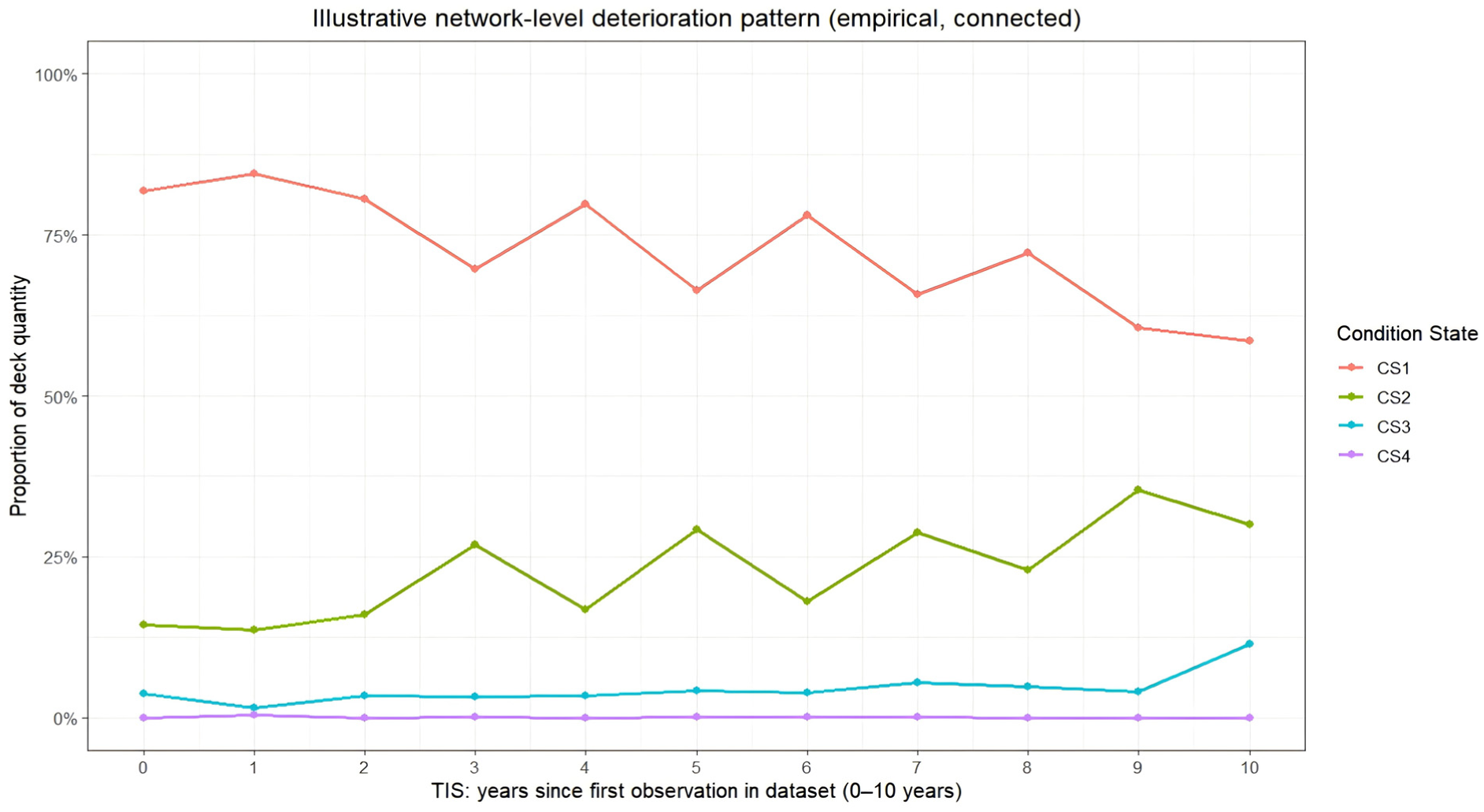
Network-level deterioration pattern over 0–10 years following the first observation in the data set (2012–2022).
This paper proposes to shift this paradigm. As a foundational step to validate this new framework, modeling efforts focus on the critical initial stages of deterioration (i.e., transitions from CS1 to CS2), where data is most abundant, and the natural degradation process can be most clearly observed.
A methodological framework is introduced that places the dynamics of element quantity transitions at the core of the deterioration modeling process. The primary contribution is not to present a definitive, production-ready deterioration model, but rather to establish and validate a novel approach that future researchers can adopt and enhance. The key innovations of this framework are twofold.
A new approach to constructing survival data: deterioration “events” are defined based on the measured transition of partial element quantities between CS (e.g., a specific area of the deck deteriorating). This novel data construction method directly harnesses the quantitative, dynamic nature of NBE data, moving beyond simple component-level ratings.
Approximation of global deterioration via weighted local events: recognizing that a partial transition is not the failure of the entire deck, an inverse probability weighted (IPW) Cox model is introduced. The weight, determined by the proportion of the element that deteriorated, allows the model to approximate the overall (global) survival characteristics of the component by aggregating these observable, localized deterioration events. This bridges the critical gap between local element-level data and component-level performance prediction (see Figure 2 for a conceptual illustration).
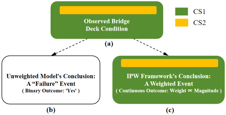
Proposed framework’s core idea compared with the traditional survival event definition: (a) observed bridge deck with partial deterioration (a portion in CS2); (b) traditional unweighted model interprets this observation as a binary “failure event”; and (c) proposed IPW framework interprets it as a continuous, weighted event, where the weight is proportional to the magnitude of the deteriorated area (weight ∝ magnitude).
To demonstrate the feasibility of this framework, a proof-of-concept study is performed on concrete bridge decks. For this initial methodological exploration, a key simplifying assumption is that only records exhibiting natural deterioration are considered, excluding instances of maintenance or repair that lead to condition improvement. This controlled approach, while not fully representative of a managed bridge network, is a necessary first step to validate the statistical integrity and behavior of the proposed IPW–Cox modeling framework in an idealized environment. This paper lays the groundwork for a new class of deterioration models that can more realistically harness the rich, quantitative information available in modern bridge inspection data.
Proposed Methodological Framework
This paper introduces a new paradigm for modeling bridge deterioration that leverages the quantitative and temporal dynamics inherent in NBE data. The framework is built on the premise that the measured transition of element quantities between CS is the most direct and informative signal of physical degradation available in routine inspection data. The proposed methodology unfolds in four conceptual steps.
Redefining deterioration events from NBE data: focus shifts from the bridge deck as a single entity to the element units that compose it. A deterioration event is no longer a binary state change for the bridge deck, but a measurable, continuous process where a quantity of an element (e.g., a specific area of the deck) transitions from a better condition state
Constructing a survival dataset from element-level changes: based on this new definition, a survival data set is constructed where each observation corresponds to a bridge element’s behavior between two inspections. The “time to event” (or survival time) is the duration the element spends in its current state, and an event is recorded if any deterioration to the next state is observed. If no change occurs, the observation is considered “right-censored.”
Applying IPW to approximate global behavior: a key challenge is that a localized event (e.g., 5% of the deck area deteriorating) does not represent the “failure” of the deck. To bridge this conceptual gap, an IPW–Cox model is employed. Each observation is assigned a weight based on the proportion of the element that transitioned. This technique allows the model to differentiate between minor and major deterioration events, using the weighted sum of local events to approximate the survival function of the component.
Fitting and validating the model: the IPW–Cox model is fitted using the constructed survival data and relevant bridge characteristics (e.g., design, age, and traffic) as explanatory variables. The model’s performance and the validity of the framework are assessed using statistical metrics (e.g., Akaike information criterion [AIC], Bayesian information criterion [BIC], and Concordance Index [C-index]) and by comparing the outcomes of weighted versus unweighted models.
This framework provides a structured pathway to extract more value from NBE data, moving beyond rating translation toward dynamic, quantitative deterioration modeling.
Data Processing
Data Source and Sample Selection
The data for this paper were sourced from the Long-Term Bridge Performance InfoBridge database, a comprehensive repository managed by the Federal Highway Administration. Concrete bridge decks were the focus because they are a critical component susceptible to various forms of deterioration. To ensure a consistent regulatory and environmental context for this proof-of-concept study, the sample was limited to bridges in Oregon. The data set encompassed NBE inspection records from 2012 to 2022 and associated NBI data, providing static bridge attributes. A critical decision in data preparation was to use NBE inspection records from 2012 onwards. This is because the NBE data specifications underwent a significant manual adjustment in 2012, where the condition state definitions were standardized from a five-state to a four-state system. Using data post-2012 ensures consistency and avoids the systemic biases that would arise from mixing pre- and post-adjustment records. The initial sample consisted of 18,197 inspection records for 1,357 distinct bridges. After applying various cleaning and filtering rules, an analysis data set of 5,784 valid data points (for
Data Processing Workflow
The transformation of raw inspection data into a structured survival data set followed the multistage workflow shown in Figure 3. This process began by merging the NBE and NBI data sources, followed by a rigorous data cleaning phase to address inconsistencies, such as missing values, duplicate records, and logical errors in element quantities. The cleaned data were then used to construct the core survival variables, which were finally supplemented by recoding categorical and continuous attributes for model input.
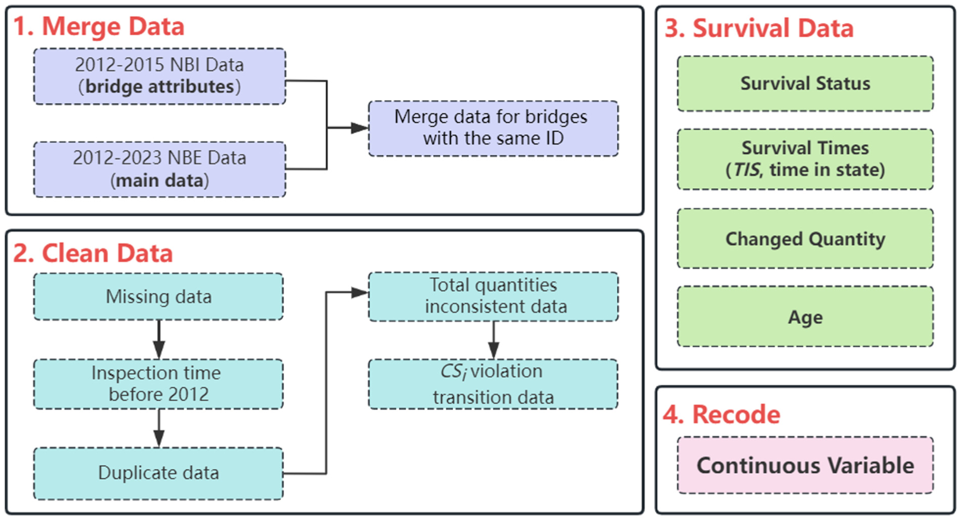
NBE data processing workflow, from raw data to a model-ready data set.
Survival Data Construction: Core of the Framework
The central innovation of this paper lies in how survival data is constructed from the NBE records. The conceptual model for this process is shown in Figure 4, which illustrates the transition of element quantities (
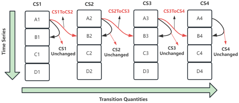
Conceptual model of element quantity transitions between condition states (CS) over time.
To operationalize the conceptual model shown in Figure 4, these dynamic transitions were translated into a set of specific variables suitable for survival analysis. The following sections detail the construction of these core variables, event status, survival time or time-in-state (TIS), and element transition quantity, which form the quantitative basis of the IPW–Cox model. Based on this model, for each bridge and for each condition state, a set of survival analysis variables between any two consecutive inspections (
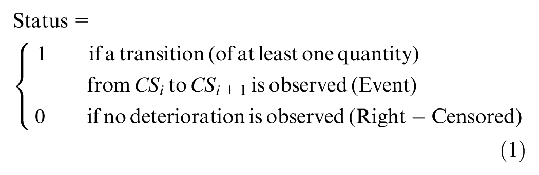
Event Status
A binary indicator, Status, was defined to identify if a deterioration event occurred. An event is registered if any quantity of the element transitions to a worse state.
Survival Time
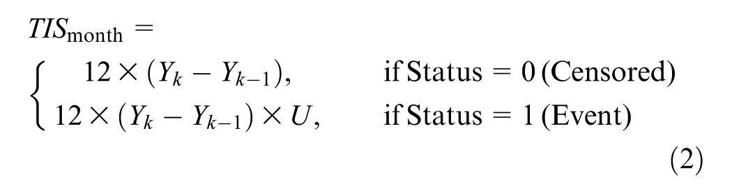
The survival time or
To construct an analyzable survival time under this data structure, the latent event time was approximated by assuming that it is uniformly distributed within the inspection interval. Under this approximation, the observed inspection interval provides the upper bound of the event time, and the realized event time is represented as a random fraction of that interval.
This approximation has important implications. Because it determines where an observed deterioration event is placed within the inspection interval, it may affect the estimated survival duration and, consequently, the shape of the baseline hazard. Its influence may be more pronounced when inspection intervals are long or highly variable across bridges. Therefore, the resulting event times should be interpreted as approximated rather than directly observed failure times.
Alternative approaches are available. For example, midpoint imputation could be used as a simpler deterministic approximation; interval-censored survival models could preserve the event time as bounded but unobserved; and multistate or event-history formulations could be adopted when denser longitudinal observations become available. These methods may provide a more rigorous treatment of transition time uncertainty; however, they would also require a different modeling framework than the one adopted in this paper.
In this paper, the primary objective is to establish and test the proposed methodological framework, which constructs survival observations directly from the NBE quantity transitions and evaluates the feasibility of the weighted Cox formulation. Within this proof-of-concept setting, the uniform-within-interval approximation provides a practical way to operationalize event timing while keeping the focus on the core methodological contribution.
where
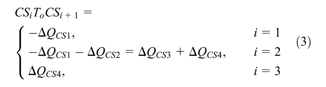
Element Transition Quantity
The element transition quantity
where
Weight Variable
The weight variable

To illustrate, consider a bridge element with 200 units (e.g., 200 ft2 of concrete deck, or 200 ft of bridge joint). If an inspection reveals that 10 of these units have transitioned to a worse CS, the weight for this observation is calculated as W = 10/200 = 0.05. This unit-agnostic approach ensures that larger deterioration events, regardless of whether they are measured in area, length, or count, have a proportionally greater influence on the model.
Bridge Age
Bridge age at the time of inspection was calculated as the inspection year minus the year the bridge was built or reconstructed.

This systematic process yields a rich data set where each row contains the survival time, event status, the magnitude of the event (as a weight), and a set of static covariates for modeling.
IPW–Cox Model
The Cox proportional hazards model (
19
) is a semi-parametric method widely used in survival analysis. The hazard function

where
The standard Cox partial likelihood function is modified to incorporate a weight
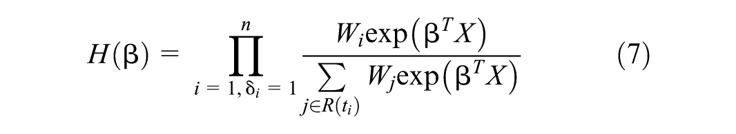
where
Explanatory Variables and Model Implementation
A set of candidate explanatory variables that may influence deck deterioration was selected from the NBI data. These included variables related to bridge age, design characteristics (e.g., main span design [MSD] and deck structure type [DST]), ownership, and traffic loading. To address the imbalance in some categorical variables, certain classes were merged based on engineering judgment, as detailed in the Appendix in Table A1.
The model-building process followed a rigorous, multistep procedure.
Initial screening: a preliminary screening of the explanatory variables was conducted using nonparametric methods, including Kaplan-Meier survival curves for qualitative assessment and log-rank tests for quantitative hypothesis testing, to identify variables with a significant effect on survival time.
Proportional hazards (PH) assumption test: all variables selected from the initial screening were formally tested for the PH assumption using the Schoenfeld residuals test (cox.zph function). Variables that violated the PH assumption (p < 0.05) were excluded from the final model to ensure its statistical validity.
Model selection: backward stepwise regression based on the AIC was used to select the most parsimonious (i.e., the simplest model that still provides adequate explanatory power) set of variables for the final model, balancing goodness-of-fit with model simplicity.
All statistical analyses were performed using the R programming language (Version 4.2.3) with the survival package.
Results
This section presents the results of the data processing and model fitting procedures objectively.
Final Data Set Characteristics
After data processing, the final data set used for modeling comprised 4,041 observations for CS1 and CS2 observations out of 5,784 data points. These were partitioned into two groups based on the initial condition state: (1) 2,786 observations for decks starting in CS1; and (2) 1,253 for decks starting in CS2. Data for CS3 were sparse (only two valid failure events were identified in this data set), and preliminary modeling attempts with CS3 data yielded unstable and unreliable results. Data for CS4 was almost non-existent (two instances remaining) because bridges in this severe state are prioritized for immediate maintenance or repair, which violates the natural deterioration assumption. Therefore, to ensure statistical robustness and model validity, CS3 and CS4 data were excluded from the final modeling.
Model Validation and Variable Selection
A critical step in validating a Cox proportional hazards model is to test the fundamental PH assumption for each covariate. This assumption states that the hazard ratio between any two individuals is constant over time. The Schoenfeld residuals test was employed (a standard diagnostic for the Cox model’s validity) to formally assess this assumption for all candidate variables.
Of note, AGE was discretized into grouped categories in the main PH-screening workflow, and average daily truck traffic (ADTT) was discretized in model specifications where traffic loading was evaluated as a candidate covariate. This modeling choice was adopted to improve interpretability and to provide a stable specification under the current event-limited and heavily right-censored data set. In addition, discretization may lead to some loss of information. To assess this issue, a sensitivity comparison between grouped and continuous specifications was conducted within the same weighted Cox framework (Appendix Table A2). The continuous specification yielded lower AIC/BIC values for CS1 and CS2, whereas the grouped specification remained comparable in concordance and global PH diagnostics; importantly, the main methodological conclusion of this paper was unchanged. The results of the PH diagnostic test for the variables included in the reported candidate model sets are presented in Table 1.
Key Variable Proportional Hazards (PH) Assumption Test Results
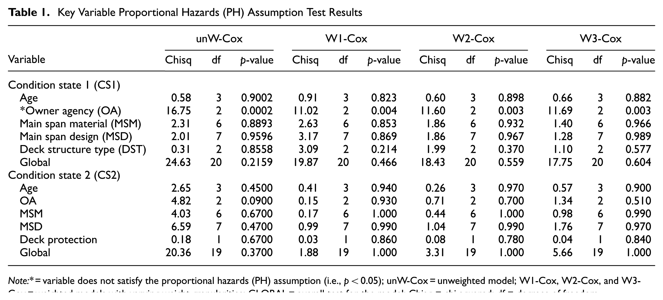
Note:* = variable does not satisfy the proportional hazards (PH) assumption (i.e., p < 0.05); unW-Cox = unweighted model; W1-Cox, W2-Cox, and W3-Cox = weighted models with varying weight granularities; GLOBAL = overall test for the model; Chisq = chi squared; df = degrees of freedom.
For CS1, the test revealed a consistent violation for the owner agency (OA) variable. Across all four models, the p-value for OA was significantly below the 0.05 threshold (e.g., p = 0.0002 for unW-Cox; p = 0.003 for W3-Cox). This finding indicates that the effect of the OA on the hazard of deterioration from CS1 is not constant over time. To maintain the statistical integrity of the final model, the OA variable was excluded from the set of candidate variables for the CS1 model fitting. All other variables, including the variable AGE, which represents the bridge age in 20-year intervals, main span material (MSM), MSD, and DST, showed p-values well above 0.05, confirming their suitability for inclusion. For CS2, Table 1 highlights that all candidate variables, including deck protection (DP), passed the PH assumption test comfortably. Of note in the weighted models (W1, W2, and W3-Cox), the p-values for all variables approached one, indicating strong compliance with the PH assumption once the weighting scheme was applied. This suggests that the IPW framework may also have a stabilizing effect on the model’s statistical properties. The GLOBAL row in Table 1 provides an overall test for the model. For all models that ultimately yielded valid results, the global p-value was well above 0.05, confirming the validity of the final set of selected variables. This rigorous diagnostic step ensures that the variables proceeding to the final model selection stage are statistically sound.
Comparative Performance of Weighting Schemes
To evaluate the efficacy of the IPW framework, four different Cox models were fitted for each condition state: an unweighted model (unW-Cox) and three weighted models (W1-Cox, W2-Cox, W3-Cox) with varying weight granularities. The W1-Cox model is the model directly weighted by the weight values from Equation 4, the W2-Cox model is the weighted model with weights recoded into ten equal intervals, and the W3-Cox model is the weighted model with weights recoded into four equal intervals. Model performance was compared using AIC, BIC, and concordance (i.e., C-index, a measure of predictive accuracy similar to an area under the curve (AUC) value). The core hypothesis of this framework, that weighting observations by the magnitude of deterioration provides a more realistic model, was tested by comparing the unweighted (unW-Cox) and weighted (W-Cox) models.
Table 2 demonstrates the superiority of the weighted approach. For CS1 and CS2, the weighted models yield significantly lower AIC and BIC values, indicating a better fit to the data while penalizing for model complexity. However, lower AIC and BIC values, while indicating superior goodness-of-fit, do not necessarily guarantee better predictive performance on new data. To address this, the model’s stability and predictive capability were further evaluated using a repeated random sub-sampling validation, as detailed in the following section. The central argument remains that the weighting scheme allows the model to better approximate the true, global deterioration process by differentiating the magnitude of localized events, a nuance that unweighted models cannot capture.
Summary of Optimal Variable Fitting Results for Different Cox Models
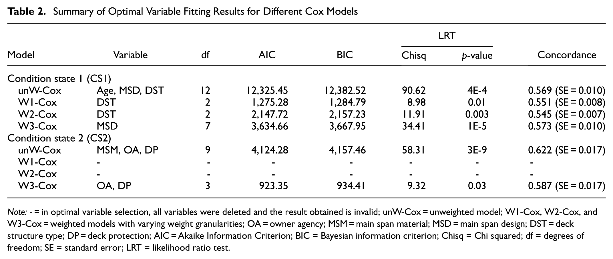
Note: - = in optimal variable selection, all variables were deleted and the result obtained is invalid; unW-Cox = unweighted model; W1-Cox, W2-Cox, and W3-Cox = weighted models with varying weight granularities; OA = owner agency; MSM = main span material; MSD = main span design; DST = deck structure type; DP = deck protection; AIC = Akaike Information Criterion; BIC = Bayesian information criterion; Chisq = Chi squared; df = degrees of freedom; SE = standard error; LRT = likelihood ratio test.
As given in Table 2, for CS1 and CS2, the weighted models produced substantially lower AIC and BIC values than the unweighted model. This indicates a superior goodness-of-fit and a lower risk of overfitting. For example, in CS1, the W3-Cox model (AIC = 3,634.66) showed a dramatic improvement over the unW-Cox model (AIC = 12,325.45).
The practical implication of this improvement is visually striking in the survival probability curves. Figure 5 shows the survival curves for the initial models fitted with all candidate variables. The unW-Cox curve is the lowest, representing the most pessimistic survival estimate. As weights are applied with increasing granularity (W1, W2, and W3-Cox), the curves systematically shift upward. This demonstrates that the IPW framework effectively corrects for the bias introduced by treating all deterioration events equally.
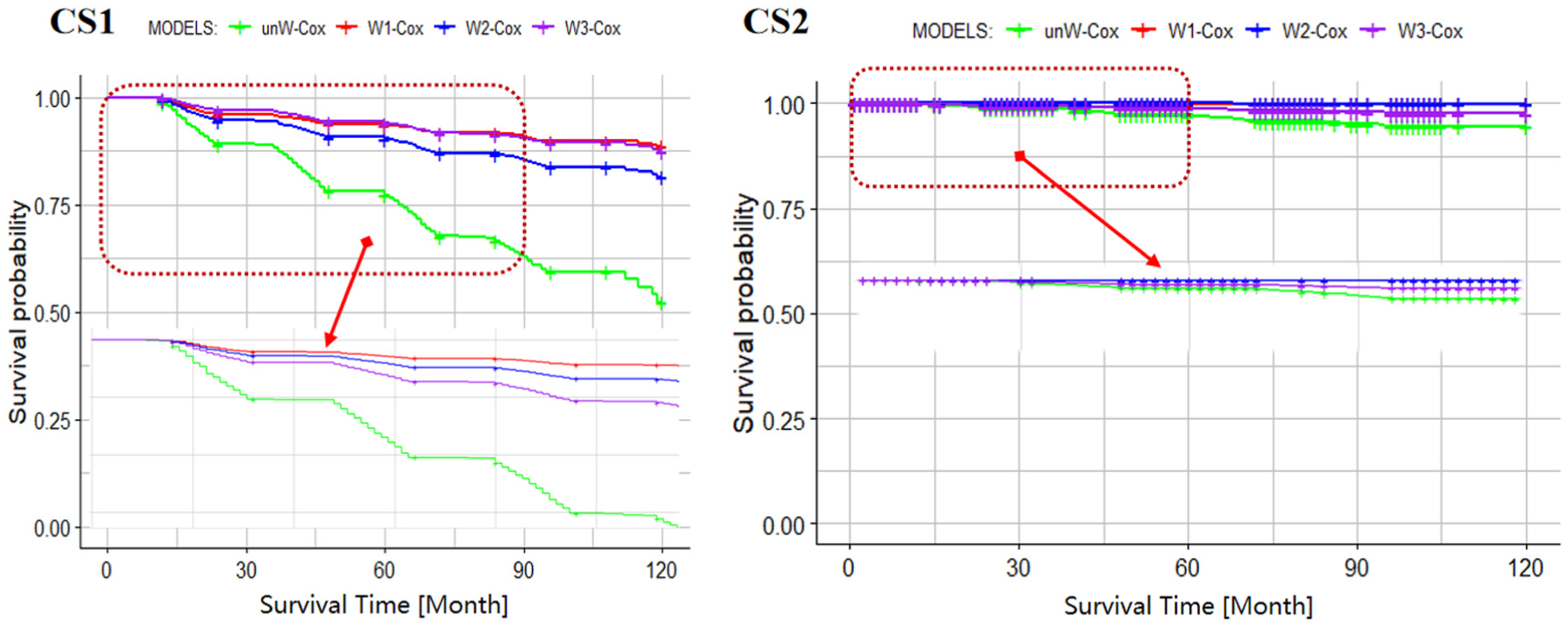
Initial survival curves for CS1 and CS2, comparing unweighted versus weighted models. The upward shift in weighted models demonstrates the core effect of the IPW framework.
This trend persists even after optimal variable selection, as shown in Figure 6. The final, more parsimonious weighted models continue to show a significantly higher survival probability than the unweighted model, confirming the robustness of the framework.
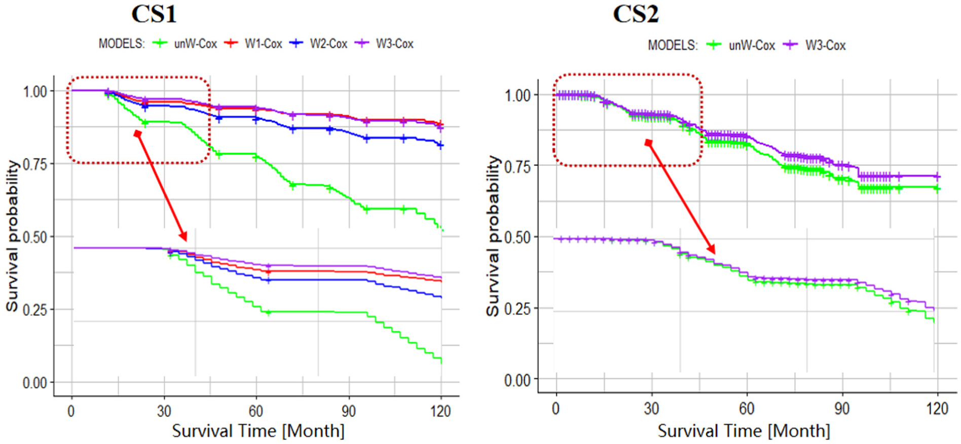
Optimal variable survival curves for CS1 and CS2. The separation between weighted and unweighted models remains, confirming the framework’s validity.
To rigorously evaluate the predictive performance and stability of the final, optimal models (W3-Cox), a cross-validation procedure was employed. Given the relatively small sample size, particularly for failure events, a standard K-fold cross-validation could lead to folds with very few or no events, resulting in fitting failures. To mitigate this, a repeated random sub-sampling validation approach was used, which is more robust for data sets with low event rates.
For each condition state (CS1 and CS2), 10 iterations of the validation were performed. In each iteration, the data was randomly partitioned into a training set (70%) and a testing set (30%). The W3-Cox model was fitted on the training set, and its predictive accuracy was evaluated on the unseen testing set. The performance was measured using two key metrics: the C-index for discriminatory power and the Brier Score for overall accuracy, which measures the mean squared error between predicted probabilities and actual outcomes. The averaged results over the 10 iterations are as follows.
For the CS1 model, the average C-index was 0.57, and the average Brier Score was 0.31.
For the CS2 model, the average C-index was 0.59, and the average Brier Score was 0.19.
The consistent performance across multiple random splits demonstrates the stability of the models.
While the C-index values are modest, this outcome is attributable to two primary factors inherent to the current stage of NBE data analysis.
First, predicting a component’s overall performance from granular element data is inherently challenging because of unobserved factors (e.g., micro-climates, specific loading histories, preservation actions). Even studies tackling simpler tasks face performance ceilings because of this stochastic nature.
Second, and perhaps more critically, the current NBE data set is limited to a 10-year observation window (2012–2022), which is significantly shorter than the typical service life of a bridge. Therefore, the data is heavily right-censored, as the majority of assets have not reached the failure threshold or exhibited significant deterioration within this narrow timeframe. This lack of observed failure events naturally constrains the model’s discriminative power.
Therefore, the C-index values should be interpreted as a confirmation that the framework captures the correct deterioration signal despite these constraints. Therefore, as longitudinal data continues to accumulate, minimizing the censoring effect, the model’s predictive accuracy will progressively improve. In addition, this framework establishes a novel methodological baseline for the NBE data set. While current predictive power is limited, this architecture is designed to scale and improve as granular maintenance records and longitudinal condition data for a much longer time horizon become available.
Final Model Parameter Estimates
In the CS2 state, a notable finding emerged: the W1-Cox (continuous weights) and W2-Cox (10-interval weights) models failed to retain any explanatory variables after the AIC-based optimal variable selection process. This is not because finer-grained weights are inherently flawed, but rather because of a critical trade-off between information granularity and model stability, especially with the smaller sample size available for CS2.
The highly granular weights in the W1-Cox and W2-Cox models probably caused the model to overfit to the specific weight values of the limited samples. The models attempted to capture minor, potentially noisy variations in the deterioration quantity, resulting in unstable coefficient estimates. Consequently, the variable selection algorithm could not identify any covariates with a robust, statistically significant effect across all observations, leading to their removal.
In contrast, the W3-Cox model, which groups weights into four broader categories (e.g., representing low, medium, high, and severe deterioration levels), sacrifices some precision for enhanced statistical robustness. This binning process effectively filters out statistical noise and allows the model to learn from the more stable, underlying signal of deterioration magnitude. This stability enabled the model to identify significant predictors and achieve a much better fit, as reflected in its superior AIC/BIC scores. Therefore, based on its statistical stability, predictive performance, and parsimony, the W3-Cox model was selected as the optimal model for the final analysis.
Table 3 presents the estimated coefficients
W3-Cox Proportional Hazard Model: Independent Variable Coefficient Analysis
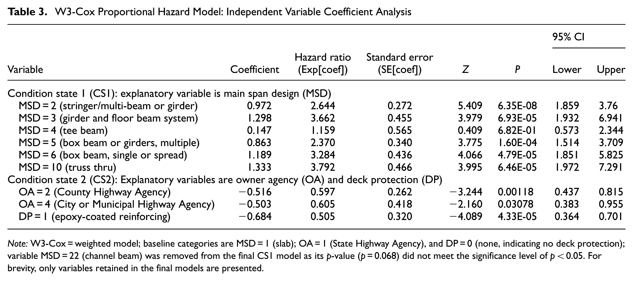
Note: W3-Cox = weighted model; baseline categories are MSD = 1 (slab); OA = 1 (State Highway Agency), and DP = 0 (none, indicating no deck protection); variable MSD = 22 (channel beam) was removed from the final CS1 model as its p-value (p = 0.068) did not meet the significance level of p < 0.05. For brevity, only variables retained in the final models are presented.
For CS1, the final model included several categories of the MSD variable, with most showing high statistical significance (p < 0.05). For CS2, the final model included OA and DP, both of which were also highly significant. The baseline hazard functions for these models were estimated and fitted using regression methods, as shown in Figure 7, with a power function providing a good fit for CS1 and a linear function for CS2.
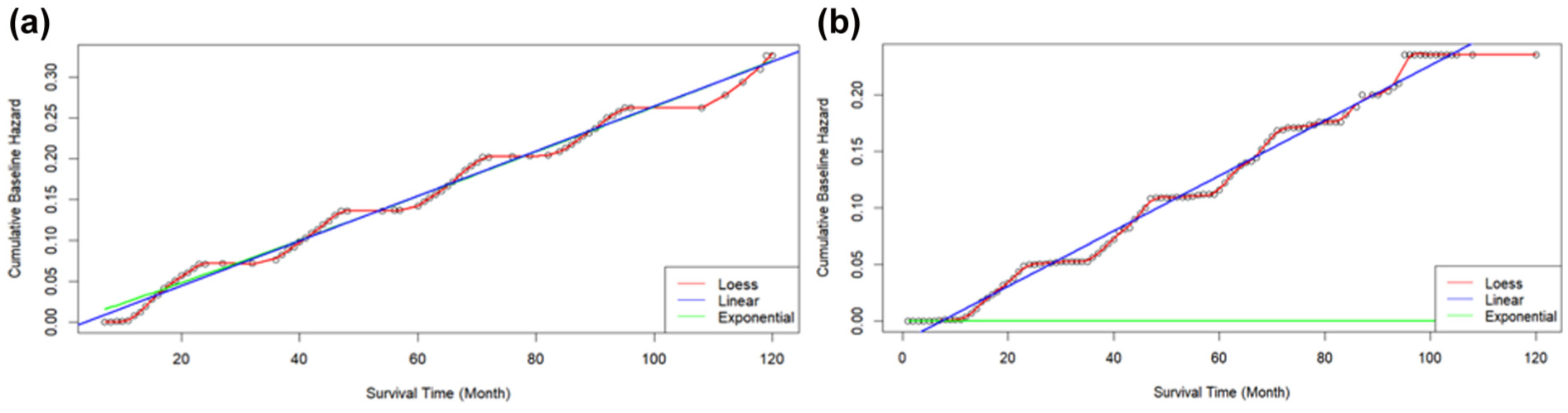
Baseline hazard function fitting for the final W3-Cox models for: (a) CS1; and (b) CS2.
Discussion
Effect of the IPW Framework on Deterioration Modeling
The results provide strong evidence for the validity and utility of the proposed methodological framework. The consistent reduction in AIC/BIC scores (Table 2) demonstrates that incorporating event-level weights significantly improves model fit. The key insight lies in the interpretation of the survival curves (Figure 6). The unweighted model treats any transition, however small, as a full failure event, leading to a pessimistic and artificially short survival time. In contrast, the IPW framework correctly interprets a small area of deterioration (e.g., 5% of the deck) as a minor event. By assigning it a smaller weight, the model’s overall hazard accumulation is reduced, resulting in a higher, more realistic survival probability curve for the entire bridge deck.
From an engineering perspective, this adjustment is not an artificial inflation but a necessary correction. The failure event is a localized process (e.g., a small area change), whereas the true failure of a bridge deck is a global process. The IPW framework correctly reflects this reality by ensuring that a minor local event contributes a small fraction to the overall hazard, providing a much more accurate approximation of the component’s true, unobservable service life. This upward shift is not an artificial inflation but a more accurate reflection of engineering reality. The framework successfully uses observable, local element changes to approximate the unobservable, global state of the component. It demonstrates a feasible pathway to bridge the conceptual gap between element-level data and component-level performance prediction.
Preliminary Insights into Deterioration Factors
While the primary goal of this paper is methodological, the final model parameters (Table 3) offer preliminary insights into factors influencing concrete deck deterioration. These insights should be interpreted with caution, given the paper’s assumptions.
CS1 (early stage deterioration): The MSD was the only significant variable. The positive coefficients for types such as “Girder and Floorbeam System” and “Truss Thru” (relative to the “Slab” baseline) suggest these designs may have a higher intrinsic hazard of initiating deterioration. This could be linked to factors such as more joints, more complex load paths, or susceptibility to water ponding, which accelerates degradation.
CS2 (developed deterioration): The significant variables were OA and DP. The negative coefficients for county/municipal ownership (relative to the state) suggest that decks under local agency management have a lower hazard (longer survival time in CS2). This is probably not because of ownership itself, but because OA serves as a proxy for different maintenance standards, traffic patterns, and inspection protocols. The negative coefficient for “Epoxy-Coated Reinforcing” is more direct, indicating its protective effect significantly reduces the hazard of further deterioration, extending the deck’s service life in CS2.
Limitations and A Roadmap for Future Research
The value of a foundational study lies in what it accomplishes and in the future research it enables. Several limitations present opportunities for subsequent work:
The “No Maintenance” assumption: This is the most significant limitation. This framework provides a baseline for natural deterioration, but it does so by excluding records with maintenance. This approach may introduce selection bias, as bridges that remain in good condition for long periods without intervention may be those in less aggressive environments or with lower traffic loads. Therefore, the resulting model might underestimate the deterioration rates for the general bridge population. The next step is to incorporate maintenance actions. This can be achieved by extending the Cox survival model to include time-dependent covariates ( 20 ), where a maintenance event (e.g., deck overlay) is introduced at the time it occurs, altering the hazard function for all subsequent periods.
Data scope and generalizability: The use of data from a single state (Oregon) limits the generalizability of the specific parameter estimates. Future work should apply this framework to a diverse set of states with varying climates, traffic loads, and maintenance practices to test the robustness of the methodology and identify regional differences in deterioration drivers.
Model formulation: The semi-parametric Cox model is a robust starting point. However, the framework can be extended to other survival model families. Parametric models (e.g., Weibull, log-logistic) could provide a closed-form expression for the baseline hazard, facilitating easier implementation. Furthermore, competing risk models could be employed to simultaneously model the probability of deteriorating to the next state versus the probability of receiving a maintenance intervention. For data sets with complex, nonlinear relationships, machine learning-based survival models such as Random Survival Forests ( 10 ) or Bayesian survival models ( 9 ) could also be explored. However, applying such advanced models is a non-trivial task that first requires the raw, time-series NBE data to be transformed into a structured survival data set with appropriate weighting. Because these models cannot be directly applied to the raw NBE data format, this framework provides this foundational step. Therefore, it is a crucial and necessary prerequisite, paving the way for future, direct benchmarking of these very state-of-the-art methods on NBE data.
Weighting scheme: This paper used a linear weighting scheme based on the proportion of transitioned area. Future research could investigate more complex, nonlinear weighting functions ( 21 ). For instance, the marginal effect of the first 5% of deck deterioration may be greater than the effect of the 50th–55th percentile. Exploring these functions could further refine the model’s accuracy.
Sensitivity of the weighting scheme: This paper employed a linear weighting scheme and categorized weights for the final model (W3-Cox) to enhance robustness. However, the IPW methodology can be sensitive to the specification of weights and the quality of the underlying data. Inconsistent data recording or unobserved maintenance actions could potentially bias the weights. The cross-validation demonstrates the robustness of the current approach for this data set; future research should explore the effect of different (e.g., nonlinear) weighting functions and advanced data cleaning techniques to ensure the framework’s reliability across diverse data sets.
Bridging the framework to practice: This paper presents a conceptual framework; its future integration into bridge management systems (BMS) holds significant promise. Current BMS often rely on binary state transitions. A model developed from this IPW framework could provide more granular predictions, such as “the probability of 5%–10% of the deck deteriorating in the next 2 years.” This level of detail could enable more nuanced decision-making, such as optimizing inspection intervals based on predicted deterioration magnitude rather than just state, or prioritizing projects that are predicted to have large, rapid transitions over those with slow, minor degradation.
Conclusion
This paper developed a methodological framework for bridge deck deterioration modeling that directly uses the dynamic quantity transitions recorded in NBE data. The framework redefines deterioration as partial CS transitions observed between inspections, constructs survival observations from these transitions, and applies an IPW–Cox model to connect localized deterioration events with component-level deterioration behavior. In the Oregon concrete deck application, the weighted models achieved better fit than the unweighted formulation and produced survival estimates that better reflect that minor local deterioration does not represent full deck-level failure. These results support the feasibility of using the NBE quantity transitions as the basis for survival-based deterioration modeling.
The direct contribution to BMS is that the proposed framework provides a practical way to convert element-level inspection records into component-level deterioration information while preserving the timing and magnitude of deterioration. Instead of relying on binary or highly aggregated condition changes, the BMS can use this output to represent how much of a deck is deteriorating and how quickly that deterioration is progressing. This creates a stronger analytical basis for deck condition forecasting, inspection planning, and project prioritization, especially when the magnitude of deterioration is important for distinguishing minor degradation from more consequential performance loss.
This implementation is based on Oregon data, the CS1–CS2 deterioration stages, and inspection records without maintenance interventions. Future work can extend the same framework by incorporating maintenance histories, broader geographic and environmental variability, and richer longitudinal inspection series. Within this scope, this paper establishes a reproducible pathway to unlock the value of NBE data in bridge deterioration analysis and to strengthen the deterioration modeling foundation of next-generation BMS.
Supplemental Material
sj-pdf-1-trr-10.1177_03611981261455030 – Supplemental material for A New Methodological Framework for Bridge Deck Deterioration Modeling Based on National Bridge Element (NBE) Data
Supplemental material, sj-pdf-1-trr-10.1177_03611981261455030 for A New Methodological Framework for Bridge Deck Deterioration Modeling Based on National Bridge Element (NBE) Data by Min Yang and Yun Bai in Transportation Research Record
Footnotes
Authors’ Note
Portions of this manuscript were refined for clarity and language using ChatGPT (OpenAI). The AI tool was used solely for language editing and polishing. All scientific content, interpretations, and conclusions are the sole responsibility of the authors.
Author Contributions
The authors confirm contribution to the paper as follows: study conception and design: Yun Bai, Min Yang; data collection: Min Yang, Yun Bai; analysis and interpretation of results: Min Yang, Yun Bai; draft manuscript preparation: Min Yang. All authors reviewed the results and approved the final version of the manuscript.
Declaration of Conflicting Interests
The authors declared no potential conflicts of interest with respect to the research, authorship, and/or publication of this article.
Funding
The authors received no financial support for the research, authorship, and/or publication of this article.
Data Accessibility Statement
The raw data used in this study are publicly available from their original sources. The processed data set generated during this study is available from the corresponding author on reasonable request. All relevant data processing steps are described within the article to support reproducibility.
Supplemental Material
Supplemental material for this article is available online.
References
Supplementary Material
Please find the following supplemental material available below.
For Open Access articles published under a Creative Commons License, all supplemental material carries the same license as the article it is associated with.
For non-Open Access articles published, all supplemental material carries a non-exclusive license, and permission requests for re-use of supplemental material or any part of supplemental material shall be sent directly to the copyright owner as specified in the copyright notice associated with the article.