Analysis of Factors Affecting Underground High-Pressure Gas Pipelines under Heavy Vehicle Loads

Abstract

As the demand for fossil fuel energy grows in China, the construction of gas pipelines has expanded significantly. These pipelines often intersect with roadways, posing critical safety risks because of potential structural failures. This study focuses on the interaction zone between high-pressure gas transmission pipelines and roads, investigating the mechanical response of pipelines under heavy vehicle loading conditions. Using Abaqus software, a pipeline-road interaction model was developed to analyze the influence of vehicle speed, load magnitude, pipe wall thickness, burial depth, and laying angles on pipeline stress distribution. The findings reveal that: heavier vehicle loads increase peak stress and vertical displacement in pipelines; higher vehicle speeds reduce these mechanical responses; pipelines installed perpendicularly (90°) to roadways exhibit minimal stress; greater burial depth reduces stress and displacement, although this effect plateaus beyond a critical depth; and thinner pipe walls amplify stress and displacement, with wall thickness being the most influential factor.

Keywords

high-pressure gas pipelines vehicle-pipeline interaction heavy vehicle loads failure analysis numerical simulations

Introduction

Natural gas is a critical global energy source, playing an indispensable role in economic development and the improvement of living standards. By 2025, China’s oil and gas pipeline network was expected to span approximately 210,000 km ( 1 ). During the rapid expansion of pipeline infrastructure, conflicts between pipelines and surrounding environments have become increasingly prominent. Rapid urbanization has created complex conditions around pipelines, with numerous intersecting highways and railways. Repeated exposure to heavy vehicle traffic may induce excessive stress and deformation in buried pipelines, potentially leading to cracking and leakage and, in severe cases, causing major safety incidents. Therefore, research on the mechanical response of buried gas pipelines under heavy vehicle loads is essential for ensuring safe pipeline operation.

Numerous studies have investigated pipeline–soil responses under surface traffic loading. Xie simplified tire–pavement contact loading under different tread patterns and showed that tread morphology can significantly affect contact pressure ( 2 ). Hui et al. analyzed the mechanical characteristics of buried pipelines considering pipe–soil contact behavior ( 3 ). Xu et al. performed pipe–soil interaction tests under subsidence and derived a simplified expression for the soil pressure at the pipe crown ( 4 ). Manolis et al. examined the dynamic response of buried pipelines in randomly structured soil using a waveguide-based framework ( 5 ). Ke et al. employed the Pasternak model and related formulations to investigate pipe–soil interaction mechanisms under external loads ( 6 ). Li et al. used finite element (FE) analysis to evaluate the three-dimensional mechanical response of buried pipelines under traffic loading ( 7 ). Chen et al. further considered vehicle speed and vehicle weight effects and proposed safety-oriented protection recommendations based on numerical results ( 8 ). In addition, field-oriented safety testing for overloaded trucks crossing underground pipelines has been reported, providing practical evidence for traffic-induced pipeline risks. Reliability and dynamic characteristics of buried pipelines subjected to traffic loading have also been studied from probabilistic and vibration perspectives. Yu et al. conducted safety tests and numerical simulations on buried pipelines crossed by overloaded trucks, finding that when the burial depth exceeds 1.5 m in uniform and dense soil, the additional stresses generated by vehicle loads are minimal and do not compromise pipeline safety ( 9 ). More recently, He et al. utilized Adams and Abaqus to establish a high-fidelity transient vehicle–road–soil–pipeline coupling model ( 10 ). Their work quantitatively analyzed the influence of various dynamic factors—including vehicle speed, internal pressure, burial depth, and wall thickness—and successfully developed a predictive model for maximum stress based on a genetic algorithm-backpropogation neural network. Zha et al. established a nonlinear contact interaction model to conduct reliability assessments of buried polyethylene pipelines under stochastic traffic loads, employing the central point method and Monte Carlo simulations to evaluate structural integrity and predict the remaining service life ( 11 ). Won et al. utilized vibration velocity as a key index for the integrity assessment of API 5L Gr. X65 pipelines, determining through FE modeling that, while the maximum vibration velocity is reached at a vehicle speed of 80 km/h, the induced vibrations remain well within the safe allowable limits for structural safety ( 12 ).

In summary, many existing studies adopt simplified static or quasi-static representations of vehicle loading, which may deviate from actual moving heavy vehicle actions. Moreover, the influencing factors of vehicle activity on buried pipelines have not been fully clarified. Current work mainly focuses on burial depth, vehicle speed, and vehicle weight, while studies on pipeline wall thickness and the crossing angle between pipelines and roadways remain relatively limited. This motivates the present study.

This paper establishes a pipe–road interaction model in Abaqus, adopts the Drucker–Prager (D-P) model to represent soil constitutive behavior under heavy loads, and investigates interaction mechanisms between pipelines and roads. Combined with the China–Myanmar Pipeline Project, FE simulations are performed to evaluate unfavorable scenarios under vehicle activity, and safety-oriented recommendations are provided for key influencing factors.

Finite Element (FE) Model

Heavy Vehicle Load Analysis

True heavy vehicle loads are stochastic and challenging to simulate in practice. Since this paper investigates the mechanical response of buried pipelines, moving vehicles are simplified as constant point source loads to verify linear motion. Therefore, a moving constant load model is selected, assuming that the load magnitude remains constant while the load position varies with time, as shown in Equation 1:

F (t) = P δ (x - vt) δ (y) H (t)

(1)

where

$F (t)$ = the time-varying force exerted on the pipeline by the moving load,

$δ (.)$ = the Dirac delta function,

x, y = the spatial coordinate,

v = the constant speed of the moving load,

t = the time variable,

$H (t)$ = the unit step function, and

$P$ = the vehicle load.

Geometry and Material Parameters

A numerical simulation model was developed using Abaqus, a nonlinear analysis software, to simulate the mechanical response of pipelines during heavy vehicle rolling operations involving backfill soil and buried pipelines. The model includes backfill soil and buried pipelines. This paper uses the China-Myanmar natural gas pipeline trunk line as the research case. Based on on-site construction data, X80 steel is selected as the pipeline material, with a density of 1,780 kg/m³, an elastic modulus of 14.4 MPa, and a Poisson’s ratio of 0.4. The pipeline parameters are set as follows: pipe diameter of 1,016 mm, wall thickness of 15.3 mm, gas transmission pressure of 10 MPa, and pipeline burial depth of 1 m. When selecting a soil model, the Mohr-Coulomb model faces challenges in calculating flow vectors, whereas the D-P model effectively addresses this issue ( 12 ). Its stress characteristics are such that, once the stress reaches the yield limit, it remains stable without further increase, while strain continues to increase. The yield criterion of the D-P model is the von Mises yield criterion, as expressed in Equations 2 and 3:

F = \sqrt{J_{2}} - α I_{1} - K = 0

(2)

J_{2} = \frac{1}{2} s_{ij} s_{ij}

(3)

where

F = the yield function,

J ₂ = the second invariant of the deviatoric stress tensor,

α = a material constant controlling the influence of the first stress invariant on yielding,

I ₁ = the first invariant of the Cauchy stress tensor (I₁ = σ_kk),

K = a material constant related to the cohesion (and frictional property) of the material, and

$s_{ij}$ = the component of the deviatoric stress tensor.

I_{1} = \frac{1}{3} σ_{kk}

(4)

Therefore, the D-P model was chosen as the soil constitutive model in Abaqus for this paper. The specific parameters are provided in Tables 1 and 2:

Table 1.

Soil Parameters

	Elasticity parameters			D-P model parameters
Category	Density (kg/m³)	Elastic modulus (MPa)	Poisson’s ratio	Angle of friction (°)	Rheological stress ratio	Expansion angle (°)
Backfill	1,780	14.4	0.4	36	1	0

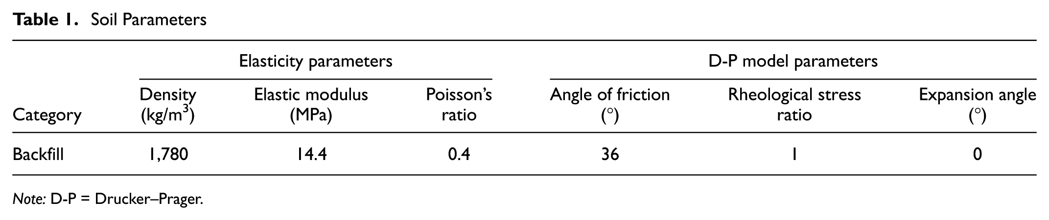
Note: D-P = Drucker–Prager.

Table 2.

D-P Model Hardening Parameters

Yield stress (MPa)	0.17	0.65	0.75	0.8	0.85
Absolute plastic strain	0	0.035	0.051	0.073	0.092

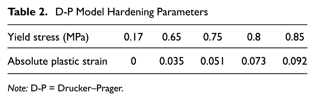
Note: D-P = Drucker–Prager.

Boundary Conditions and Meshing

To ensure isotropic mechanical responses under heavy vehicle rolling load test conditions, the model includes pipeline internal pressure, pipeline self-weight, soil gravity, and the external vehicle load. The soil is modeled as an isotropic, homogeneous continuum with dimensions of 20 m (length) × 4 m (width) × 7.5 m (height). This soil domain is selected to minimize the influence of artificial boundaries on the pipe–soil coupled response by providing sufficient distance from the pipeline and the wheel-loading zone to the lateral and bottom boundaries, so that displacement and stress disturbances decay markedly before reaching the boundaries, thereby avoiding boundary-induced stress concentration or an unrealistically stiff response. With the pipeline outer diameter D = 1.016 m as a reference, the domain length, width, and height are approximately 20D, 4D, and 7.4D, respectively, which enables the dominant stress diffusion and local pipe deformation under the rolling load to develop fully while maintaining a reasonable computational cost.

The pipeline burial depth is set to 1 m, consistent with commonly adopted cover depths for buried pipelines under roadway traffic conditions. This choice captures both the load-spreading effect through the soil cover and the confinement characteristics of the surrounding ground, ensuring that the additional stresses induced by wheel loading are representative. The pipeline outer diameter of 1,016 mm is a typical large-diameter specification for long-distance high-pressure gas transmission pipelines and is therefore selected to represent trunkline behavior under vehicle-crossing scenarios. The wall thickness of 15.3 mm is chosen in accordance with commonly used engineering wall-thickness grades, such that the circumferential stiffness and local bending resistance fall within practical ranges, facilitating the applicability of the simulation results. The operating pressure is set to 10 MPa to reflect a typical in-service internal pressure level for high-pressure gas pipelines; the internal pressure introduces significant hoop membrane stress and alters the overall stress state of the pipe wall, thereby affecting stress superposition and deformation patterns under vehicle loading, and is therefore retained to improve the realism of the modeled service condition.

The vehicle load is applied to the soil surface, and the pipeline is oriented perpendicular to the vehicle’s travel path, as shown in Figure 1. In Abaqus, U1, U2, and U3 represent the translational displacement components along the global 1-, 2-, and 3-directions of the model coordinate system, respectively. Accordingly, boundary conditions are imposed on the soil domain with constraints in the U1 direction on the left and right sides, in the U3 direction on the front and rear sides, and in the U1, U2, and U3 directions on the bottom surface to restrain rigid-body motion and to approximate the confinement provided by the far-field ground. Displacement/rotation boundary conditions are applied in the U3 direction at both ends of the pipe to represent end restraint from adjacent pipeline segments and to ensure stable numerical response under the moving load. Face-to-face contact is defined between the pipe and the soil, with the normal behavior of the contact surface set to “hard contact” and the constraint enforcement method set to the default option. The tangential behavior is set to “penalty” in all directions, with a friction coefficient of 0.3 to represent the pipe–soil interface friction during loading.

Figure 1.

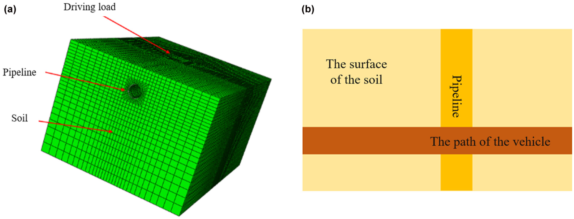
Finite element (FE) simulation diagram: (a) FE diagram of the model and (b) schematic diagram of the distribution of the upper surface of the soil.

The soil is discretized using C3D8R elements, while the pipeline is modeled with S4R elements. The pipeline is constructed through extrusion in “shell” mode, while the soil is modeled using “solid” extrusion. To enhance simulation accuracy, the soil elements around the pipeline are refined. At the same time, computational efficiency is maintained by coarsening the mesh in regions distant from the pipeline.

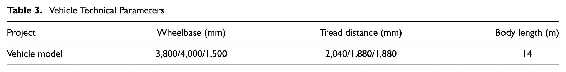
Under real-world conditions, tire pressure distribution is asymmetric, and vehicle loading patterns are random. To enhance the realism of the test and facilitate calculations, the vehicle loading pattern is simplified as follows: it is assumed that the contact area between the tire and the road surface remains constant at each moment of contact, and the vehicle load is treated as a moving constant load, with the force magnitude remaining unchanged. Based on the statistics of the primary vehicles crossing the road along the China-Myanmar Pipeline, a five-axle truck was selected as the research subject. According to the Design Standards for Medium and Heavy-Duty Cargo Vehicles ( 13 ), the key vehicle parameters are presented in Table 3.

Table 3.

Vehicle Technical Parameters

Project	Wheelbase (mm)	Tread distance (mm)	Body length (m)
Vehicle model	3,800/4,000/1,500	2,040/1,880/1,880	14

The current principal component analysis method is used to approximate the wheel contact area as a rectangle with dimensions 0.8712L × 0.6L, where L represents the vehicle length. The distribution of all wheel contact areas is shown in Figure 2.

Figure 2.

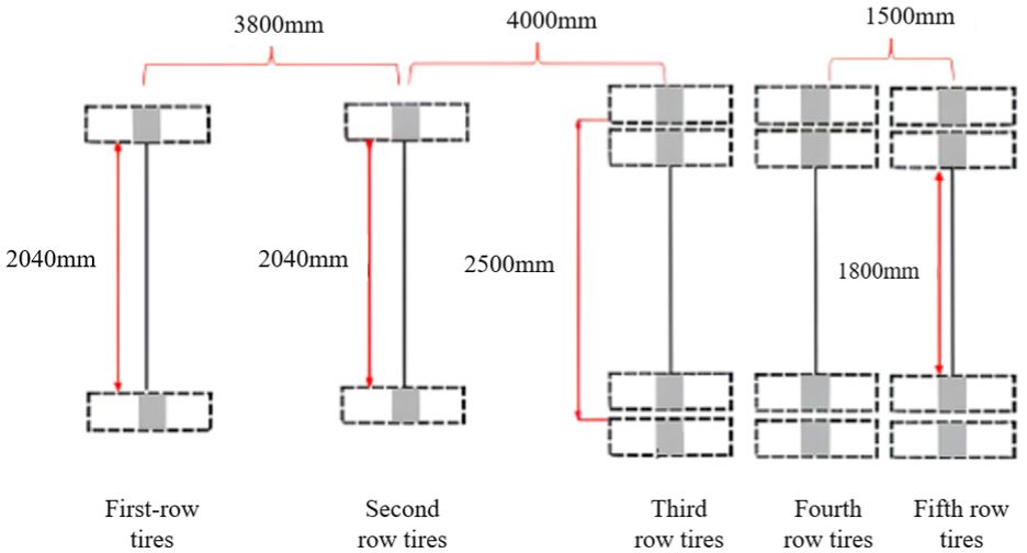
Schematic diagram of the distribution of wheels to the ground.

The dimensions of the moving load zone were defined as follows: its width equals the tire contact area, and its length corresponds to the vehicle’s travel distance. The moving load zone was aligned with the direction of travel and discretized into contiguous rectangular segments, as shown in Figure 3.

Figure 3.

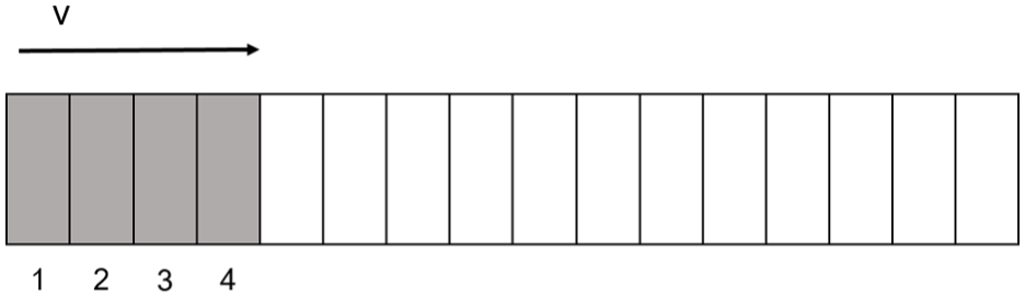
Schematic diagram of moving belt division.

The area of the first four rectangles in Figure 3 represents the initial tire force application area when the vehicle load is first applied. As the vehicle moves forward, multiple load steps are defined to apply continuous rectangular forces from the tires to the road surface, simulating the movement of the vehicle load. The movement speed of the vehicle load is controlled by adjusting the duration of each load step.

The Abaqus/Explicit module provides several subroutines to accommodate user-specific analysis requirements. To simulate moving wheel loads, the DLOAD subroutine was used to define the vertical ground contact load.

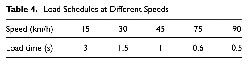
When programming the DLOAD subroutine in Fortran, parameters such as the load application distance, start and end positions, and the time for each wheel of the vehicle must be defined. The starting point is defined as the horizontal distance of 2 m from the top of the pipeline to the contact surface of the front wheels with the road. The endpoint is when the rear-axle wheels are at a horizontal distance of 2 m from the top of the pipeline, with the vehicle having traveled a total distance of 16 m. The loading times for moving loads at different vehicle speeds are detailed in Table 4.

Table 4.

Load Schedules at Different Speeds

Speed (km/h)	15	30	45	75	90
Load time (s)	3	1.5	1	0.6	0.5

The vehicle rolling load analyzed in this study is a moving load. To simulate this dynamic interaction, the Abaqus/Explicit module was used, and the DLOAD subroutine was selected to apply the moving load.

Validation of Finite Element (FE) Models

To verify the accuracy and reliability of the proposed FE model, a validation study was carried out based on previously reported experimental measurements and analytical calculations for soil stress under surface loading. Specifically, Abaqus was used to simulate the soil stress distribution at different burial depths in a soil-only configuration (i.e., without a pipe) under the same loading scenario, so that the stress attenuation with depth could be directly compared with the available measured/calculated results reported in the literature ( 9 – 12 ). The soil stress contours were first obtained from the FE model, and the stress values at target depths were extracted for quantitative comparison.

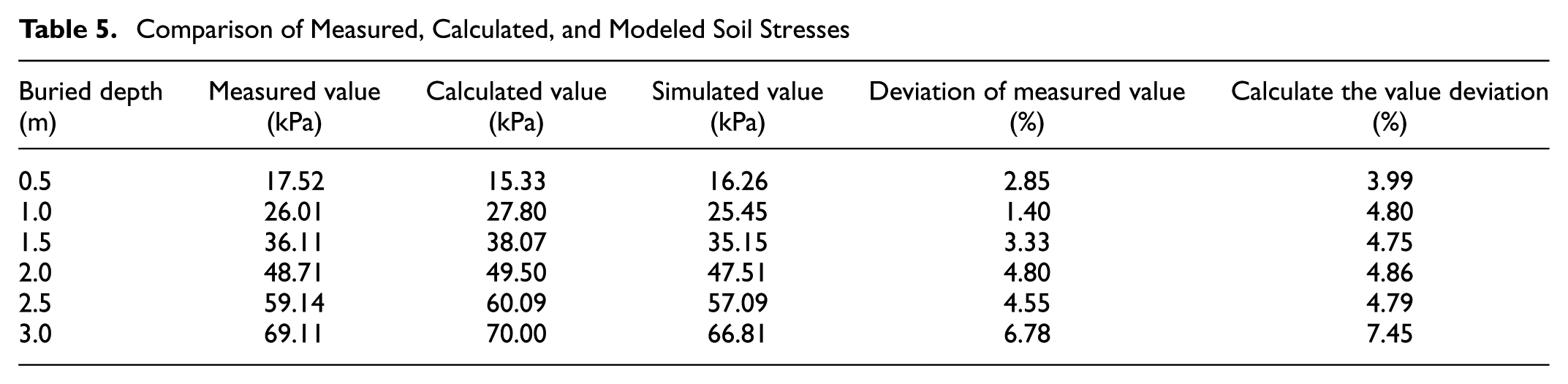
The validation considered burial depths of 0.5, 1.0, 1.5, 2.0, 2.5, and 3.0 m, and the corresponding FE-predicted soil-layer stresses are summarized in Table 5, together with the reference measured and calculated values. Overall, the FE results show good agreement with the reference data across all depths. The maximum relative error between the simulated and reference values is 7.45%, while the minimum relative error is 1.40%, indicating that the FE model captures the depth-dependent stress transfer and attenuation behavior with satisfactory accuracy. Therefore, the adopted modeling strategy (i.e., material representation, boundary constraints, and contact definition) is considered valid, and the subsequent parametric analyses of pipeline responses under vehicle loads are based on a reasonably accurate numerical framework.

Table 5.

Comparison of Measured, Calculated, and Modeled Soil Stresses

Buried depth (m)	Measured value (kPa)	Calculated value (kPa)	Simulated value (kPa)	Deviation of measured value (%)	Calculate the value deviation (%)
0.5	17.52	15.33	16.26	2.85	3.99
1.0	26.01	27.80	25.45	1.40	4.80
1.5	36.11	38.07	35.15	3.33	4.75
2.0	48.71	49.50	47.51	4.80	4.86
2.5	59.14	60.09	57.09	4.55	4.79
3.0	69.11	70.00	66.81	6.78	7.45

Analysis of the Influence of Heavy Vehicle Load on Buried Gas Pipelines

Stress Response Analysis of Pipes

A vehicle weighing 60 tons and traveling at 30 km/h was selected and incorporated into the model for calculation. The maximum von Mises stress distribution curves of the pipeline under varying vehicle distances are shown in Figure 4. It can be observed that the maximum von Mises stress on the pipeline varies with the driving distance. The closer the pipeline is to the horizontal distance above the tire, the greater the maximum von Mises stress it experiences. Since the research subject is the China-Myanmar high-pressure natural gas pipeline, the pipe diameter is set at 1,016 mm, and the pipeline pressure is 10 MPa. Based on existing literature, this study considers only the following factors: vehicle speed, vehicle weight, pipeline wall thickness, burial depth, and pipeline laying angle (i.e., the angle between the pipeline crossing the road and the road surface, as shown in Figures 3 –8) ( 14 ). The study focuses on the scenario in which the pipeline is most affected, specifically when the third row of tires passes directly above the pipeline.

Figure 4.

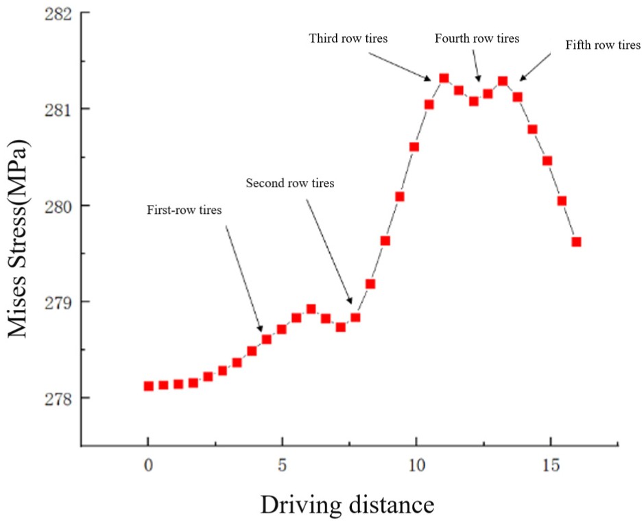
Trend chart of maximum pipe stress with vehicle distance.

Figure 5.

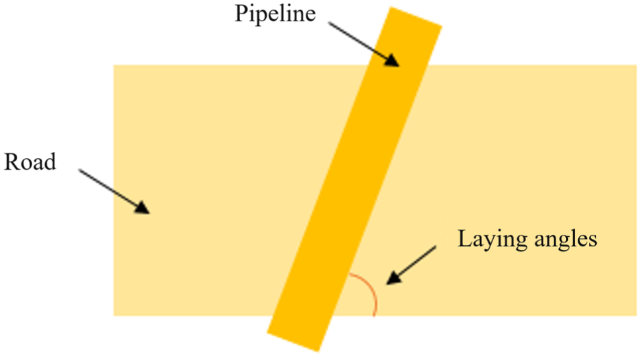
Schematic diagram of pipe laying angle.

Figure 6.

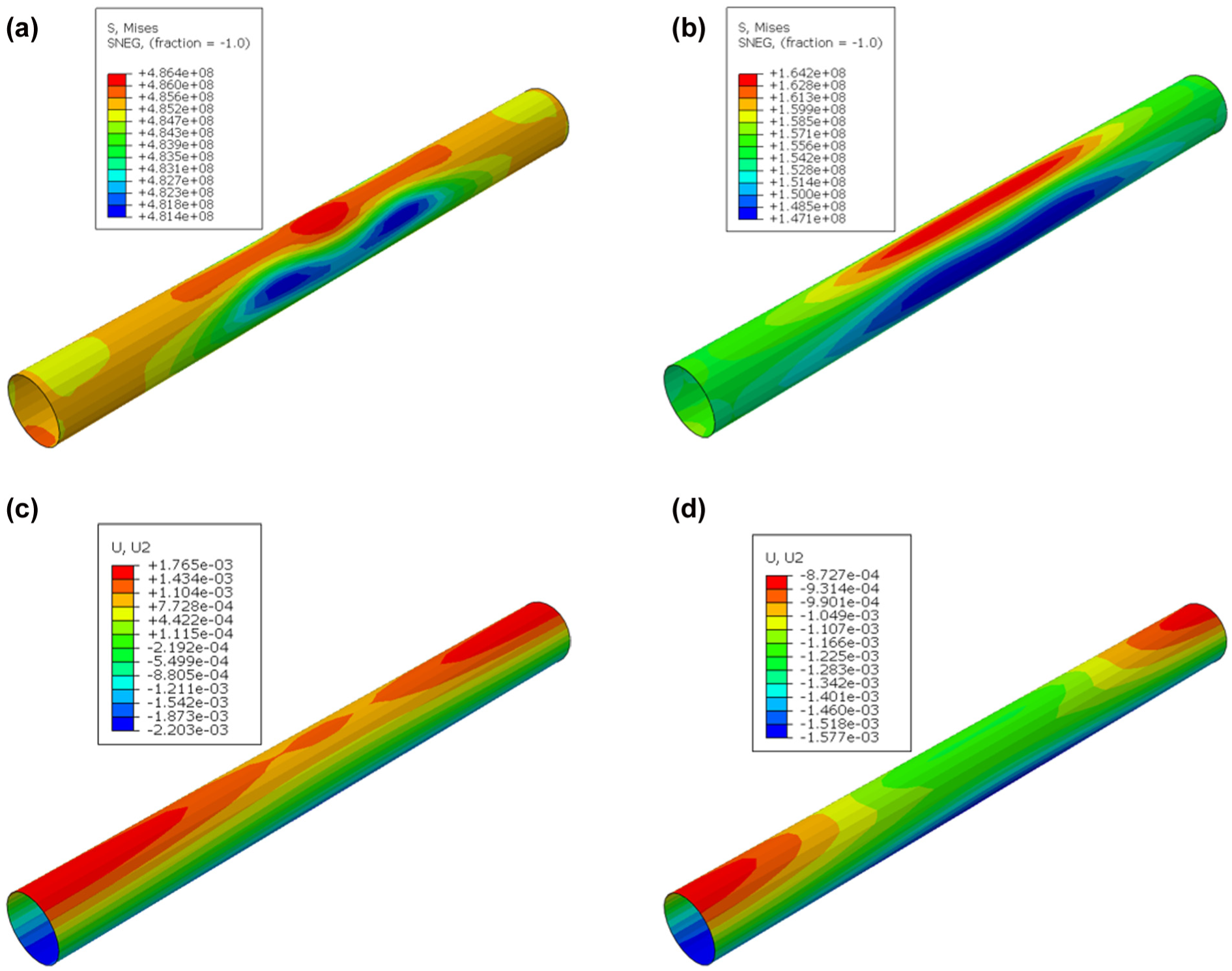
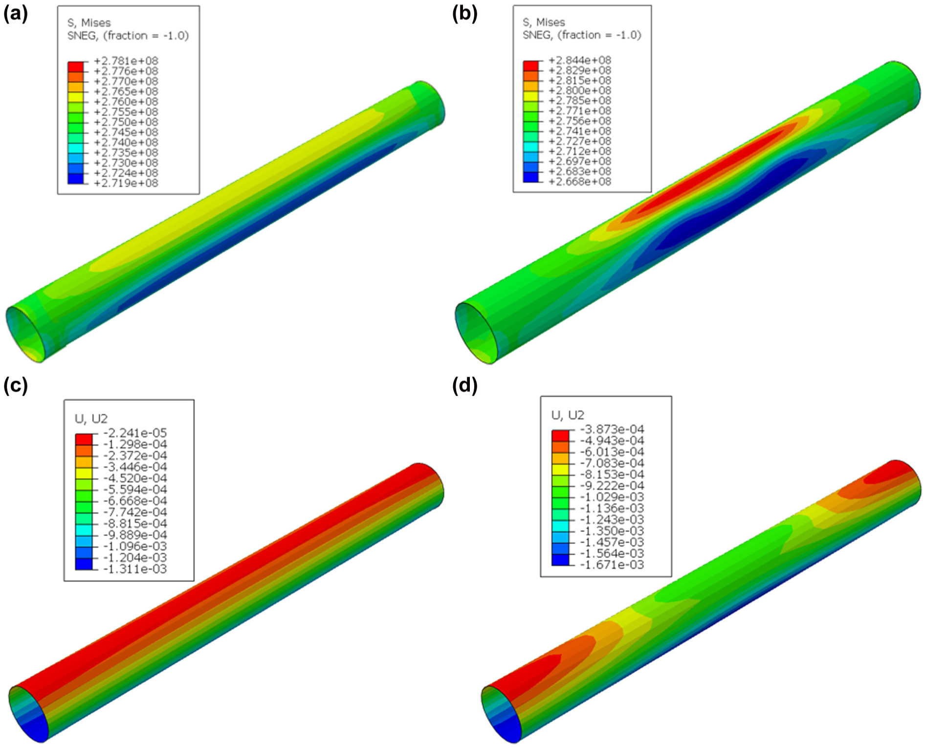
Simulated cloud view of the pipe with different wall thicknesses: (a) wall thickness 9 mm, pipe Mises stress diagram, (b) wall thickness 28 mm, pipe Mises stress diagram, (c) wall thickness 9 mm, vertical displacement diagram of pipe, and (d) wall thickness 28 mm, vertical displacement diagram of pipeline.Note: S. Mises represents von Mises stress; U2 represents the vertical displacement of the pipe. SNEG refers to the negative surface of the shell element in the simulation output.

Figure 7.

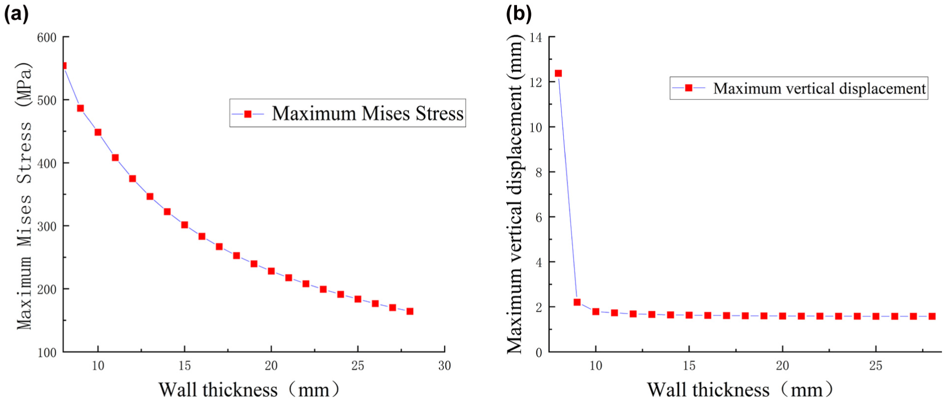
Pipe response under different wall thicknesses: (a) diagram of the relationship between the maximum Mises stress and wall thickness and (b) relationship between maximum vertical displacement and wall thickness.

Figure 8.

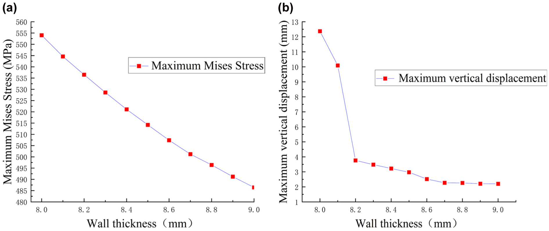
Pipe response diagram under 8–9 mm wall thickness: (a) diagram of the relationship between the maximum Mises stress and wall thickness and (b) relationship between maximum vertical displacement and wall thickness.

Analysis of the Influence of Pipeline Wall Thickness on Buried Gas Pipelines

Different pipe wall thicknesses were selected to study their effects on the pipe von Mises stress and vertical displacement. A vehicle with a mass of 75 tons and a speed of 60 km/h was adopted, with all other conditions held constant and only the pipe wall thickness varied. The wall-thickness range was set from 8 to 28 mm. The lower and intermediate thickness levels were chosen to represent commonly used wall-thickness grades in engineering practice, whereas the upper limit of 28 mm was introduced to provide a thick-wall upper-bound case that may occur under traffic crossings, high-consequence areas, or conservative design conditions, where wall thickness is jointly governed by design internal pressure, steel grade, corrosion allowance, and safety factors. Extending the thickness range also enables a clearer sensitivity assessment and allows potential attenuation of response and “diminishing returns” behavior with increasing thickness to be identified, thereby improving the generality of the conclusions. Moreover, under the same pipe diameter, burial depth, soil properties, and loading conditions, 28 mm remains within a thickness range that permits stable meshing and contact convergence, ensuring numerical stability and comparability across cases. FE simulations were performed for the above configurations, and the results for different wall thicknesses are presented in Figures 6 and 7.

As shown in Figure 7a, under the same conditions, the thinner the pipe wall, the greater the maximum von Mises stress on the pipe. As shown in Figure 7b, the maximum vertical displacement of the pipe varies significantly between wall thicknesses of 8 and 9 mm. The maximum vertical displacement of a pipe with a wall thickness of 9 mm is 2.203 mm, while that of a pipe with a wall thickness of 8 mm is 12.37 mm, representing a growth rate of 561.5%. The thinner the pipe wall, the greater the potential danger. A detailed study was conducted on wall thicknesses between 8 and 9 mm, and the pipe simulation results are shown in Figure 6. Further analysis of Figure 6 reveals that the maximum von Mises stress and maximum vertical displacement decrease as the wall thickness increases. The maximum vertical displacement changed significantly between pipe wall thicknesses of 8.1 and 8.2 mm. The maximum vertical displacement of the 8.1 mm wall thickness pipe was 10.09 mm, while that of the 8.2 mm wall thickness pipe was 3.761 mm. This vertical displacement variation is related to the plasticity parameters of the pipeline. When the plastic stress of the pipeline reaches the yield limit, the pipeline undergoes severe deformation.

Further analysis of Figure 8 reveals that the maximum von Mises stress and maximum vertical displacement decrease as the wall thickness increases. The maximum vertical displacement changed significantly between pipe wall thicknesses of 8.1 and 8.2 mm. The maximum vertical displacement of an 8.1 mm wall thickness pipe is 10.09 mm, while that of an 8.2 mm wall thickness pipe is 3.761 mm. This vertical displacement variation is related to the plasticity parameters of the pipeline. When the plastic stress of the pipeline reaches the yield limit, the pipeline undergoes severe deformation.

Analysis of the Influence of Buried Depth of Pipelines on Buried Gas Pipelines

Different burial depths were selected to study their effects on the von Mises stress and vertical displacement of the pipeline. A vehicle with a mass of 75 tons and a speed of 60 km/h was used, with all other conditions held constant and only the burial depth varied. To investigate the influence of burial depth on buried gas pipelines, a range of burial depths from 0.6 to 5.0 m was selected for the study. The simulated partial cloud maps of the pipeline under different burial depths are shown in Figure 9, and the pipeline response diagrams are shown in Figure 10.

Figure 9.

Simulated cloud image of pipeline at different burial depths: (a) buried depth of 0.6 m, and Mises stress contour of pipeline, (b) buried depth of 1.2 m, and Mises stress contour of pipeline, (c) buried depth of 0.6 m, vertical displacement diagram of pipeline, and (d) buried depth of 1.2 m, vertical displacement diagram of pipeline.Note: S. Mises represents von Mises stress; U2 represents the vertical displacement of the pipe. SNEG refers to the negative surface of the shell element in the simulation output.

Figure 10.

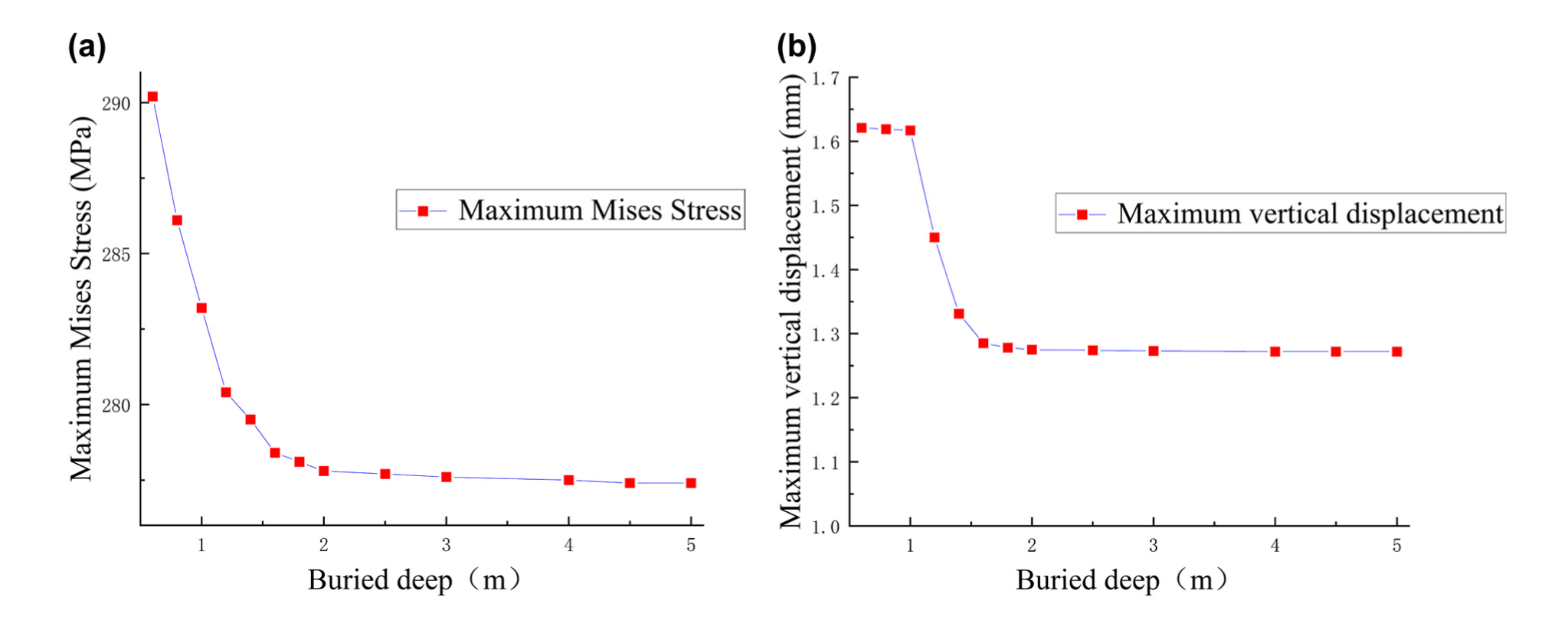
Plot of pipe response under different burial depth conditions: (a) diagram of the relationship between the maximum Mises stress and the buried depth and (b) relationship between maximum vertical displacement and burial depth.

As shown in Figure 10, the maximum von Mises stress decreases significantly as burial depth increases from 0.6 to 2.0 m. The maximum vertical displacement decreases significantly when burial depth increases from 1.0 to 2.0 m. Beyond a burial depth of 2.0 m, further increases in burial depth result in minimal changes in both maximum von Mises stress and maximum vertical displacement.

For pipelines buried at depths less than 2.0 m, increasing the burial depth significantly mitigates the adverse effects of vehicle-induced stress. However, for burial depths greater than 2.0 m, further increases have a negligible impact on reducing vehicle-induced stress.

Analysis of the Influence of Pipeline Laying Angle on Buried Gas Pipelines

Different pipe laying angles were selected to study their effects on pipe von Mises stress and vertical displacement. A vehicle with a mass of 75 tons and a speed of 60 km/h was used, with all other conditions held constant and only the pipe laying angle varied. A total of six pipe laying angles were set: 90°, 75°, 60°, 45°, 30°, and 15°. The dynamic response of buried pipes under these six operating conditions was analyzed, and fitting curves were plotted, as shown in Figure 11.

Figure 11.

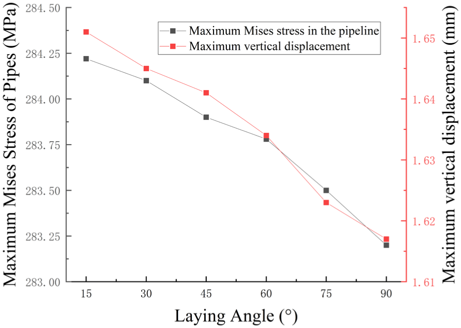
Diagram of maximum Mises stress and maximum vertical displacement of pipeline at different laying angles.

As shown in Figure 11, the closer the laying angle is to 90°, the smaller the maximum von Mises stress and maximum vertical displacement of the pipeline. Therefore, pipelines crossing roads should be laid as perpendicular to the road as possible.

Analysis of the Influence of Vehicle Weight on Buried Gas Pipelines

Only the vehicle weight is varied, with a driving speed of 60 km/h selected and all other parameters held constant. Five operating conditions are set with vehicle weights of 30, 45, 60, 75, and 90 tons. Using Abaqus software simulation, the partial stress maps of the pipeline under different vehicle weights are shown in Figure 12. The maximum von Mises stress and maximum vertical displacement of the buried pipeline as a function of vehicle weight and their trends are shown in Figure 13.

Figure 12.

Simulation cloud of pipeline under different vehicle weights: (a) vehicle weight of 30 tons, pipeline Mises stress diagram, (b) vehicle weight of 90 tons, pipeline Mises stress diagram, (c) vehicle weight of 30 tons, vertical displacement diagram of pipeline, and (d) vehicle weight of 90 tons, vertical displacement diagram of pipeline.Note: S. Mises represents von Mises stress; U2 represents the vertical displacement of the pipe. SNEG refers to the negative surface of the shell element in the simulation output.

Figure 13.

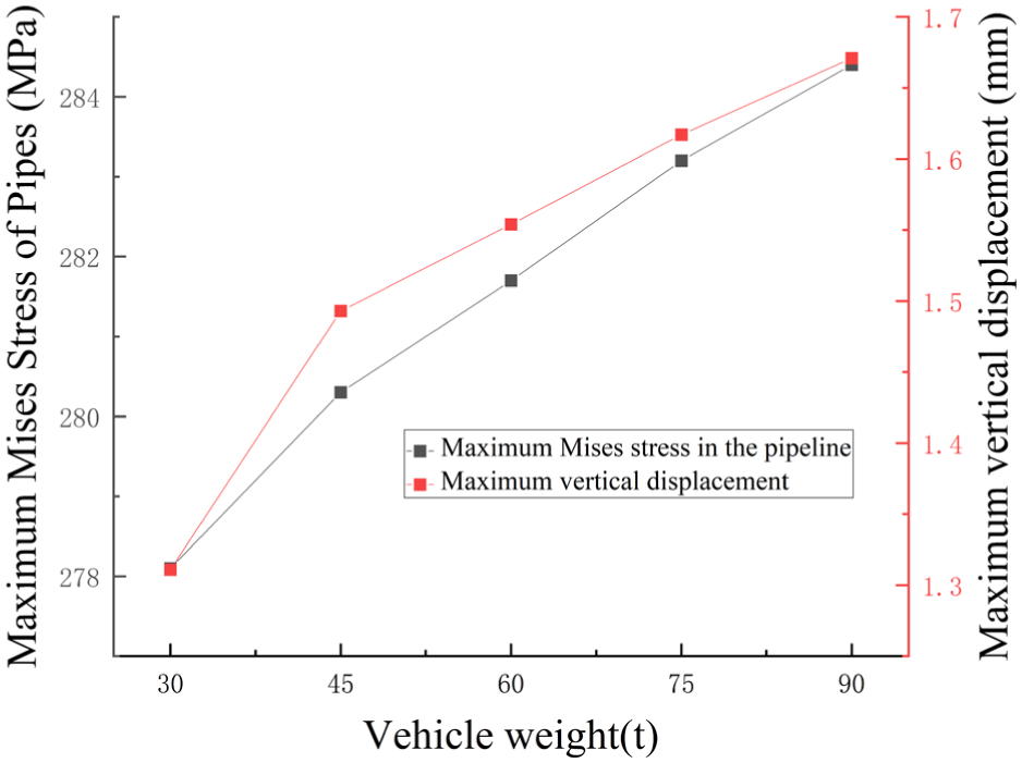
Diagram of maximum Mises stress and maximum vertical displacement of pipe under different vehicle weights.

The results show that, as the vehicle weight increases, the maximum von Mises stress and maximum vertical displacement of the pipe also increase accordingly. When the vehicle weight increased from 30 to 90 tons, the maximum von Mises stress increased from 278.1 to 284.4 MPa, and the rate of increase remained consistent with the increase in vehicle weight. When the vehicle weight increased from 30 to 90 tons, the maximum vertical displacement increased from 1.311 to 1.671 mm, with the fastest rate of increase occurring in the 30–45 tons range.

Analysis of the Influence of Vehicle Speed on Buried Gas Pipelines

Only the vehicle speed is varied, with a vehicle weight of 60 tons and all other model parameters held constant. Simulations were conducted for vehicle speeds ranging from 10 to 90 km/h, and the variation in the maximum von Mises stress and maximum vertical displacement of the buried pipeline with respect to vehicle speed, along with their trends, are shown in Figure 14.

Figure 14.

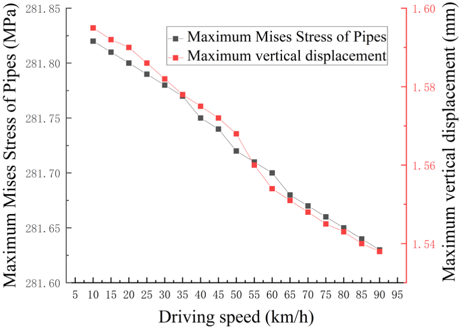
Trend plot of maximum Mises stress of pipeline with vehicle speed.

As shown in Figure 14, with an increase in vehicle speed, the maximum von Mises stress and maximum vertical displacement of the pipeline exhibit a decreasing trend. When the vehicle speed increases from 10 to 90 km/h, the maximum von Mises stress decreases from 281.82 to 281.63 MPa, and the maximum vertical displacement decreases from 1.595 to 1.538 mm. This suggests that low-speed driving contributes to increased pipeline damage.

Conclusions

In summary, this study focuses on high-pressure gas transmission pipelines and evaluates the mechanical response of buried pipelines subjected to heavy vehicle activity in pipeline–road interaction zones. By systematically varying key factors (i.e., wall thickness, burial depth, laying angle, vehicle mass, and vehicle speed) while maintaining consistent boundary and contact conditions, the results provide a quantitative basis for identifying dominant risk drivers and for prioritizing practical mitigation measures in traffic crossing sections.

1) Stress response and governing factors. Under heavy vehicle loading, the maximum von Mises stress increases notably as wall thickness decreases and as vehicle mass increases, indicating that structural stiffness and axle load demand are primary drivers of stress amplification. Increasing burial depth generally reduces the maximum stress; however, once the burial depth exceeds approximately 2.0 m, the marginal reduction becomes limited, suggesting a diminishing-return behavior for further deepening under the studied conditions. With respect to pipeline–road geometry, a laying angle closer to 90° yields smaller maximum stress, indicating that near-perpendicular crossings can reduce adverse bending and stress concentration induced by surface loading. The parametric results also show that vehicle speed influences the transient response, but its effect should be interpreted in the context of traffic safety and real-world controllability.

2) Deformation response and sensitivity. The maximum vertical displacement increases markedly as wall thickness decreases, and a pronounced sensitivity is observed between 8 and 9 mm, where the 8 mm case exhibits a maximum displacement approximately 5.6 times that of the 9 mm case. This highlights a critical thickness threshold within the investigated range, below which deformation escalates rapidly and serviceability risk may dominate. Similar to the stress response, increasing burial depth reduces vertical displacement but shows limited additional benefit beyond approximately 2.0 m. A laying angle approaching 90° reduces vertical displacement, and heavier vehicles increase displacement. These trends collectively indicate that both structural stiffness (i.e., wall thickness) and traffic load intensity (i.e., vehicle mass) are the most influential and practically addressable factors.

3) Integrated engineering implications and recommendations. The combined results suggest that effective risk control for pipeline–road crossings should prioritize 1) maintaining sufficient structural capacity (i.e., avoiding overly thin walls in heavy-traffic crossings), 2) selecting a burial depth that provides meaningful load attenuation without unnecessary construction cost, and 3) adopting near-perpendicular crossing geometry whenever feasible. Based on the observed diminishing-return behavior beyond 2.0 m, a burial depth exceeding 1.2 m is recommended as a minimum safety-oriented measure in the studied scenario, while recognizing that increasing depth beyond approximately 2.0 m may yield limited additional benefit for stress and displacement reduction. For operational management, the most practical and enforceable measures are preventing truck overloading (axle-load control) and implementing traffic management policies at crossings where pipelines are vulnerable. Because specifying a minimum vehicle speed is generally not feasible or safe in real traffic operations, this study does not recommend a target minimum speed; instead, risk mitigation should rely on load control, appropriate crossing design (i.e., near 90°), and, where necessary, additional protective measures (e.g., improved backfill/compaction, local reinforcement, or protective slabs) to reduce the pipeline response under heavy vehicle passages.

Footnotes

Authors’ Note

During the preparation of this work, the authors used ChatGPT-4 for the purpose of improving language and readability. After using this tool/service, the authors reviewed and edited the content as needed and take full responsibility for the content of the publication.

Author Contributions

The authors confirm contribution to the paper as follows: study conception and design: R. Hongwei, Z. Kai; data collection: L. Yang; analysis and interpretation of results: C. Liqiong, J. Haoyu; draft manuscript preparation: R. Hongwei, Z. Kai. All authors reviewed the results and approved the final version of the manuscript.

Declaration of Conflicting Interests

The authors declared no potential conflicts of interest with respect to the research, authorship, and/or publication of this article.

Funding

The authors received no financial support for the research, authorship, and/or publication of this article.

ORCID iDs

Rao Hongwei

Jia Haoyu

References

Gao

Zhang

Gao

New Progress in China’s Oil and Gas Pipeline Construction in 2022. International Petroleum Economics, Vol. 31, No. 3, 2023, pp. 16–23.

Xie

S. Y.

Influence of Vehicle Load on Asphalt Pavement Distress. Journal of Zhejiang Institute of Communications, Vol. 9, No. 1, 2008, pp. 5–7, 33.

Hui

Wang

Lei

Xuan

Wang

Chen

Analysis on Mechanical Characteristics of Buried Pipeline under Pipe-Soil Contact. Oil Field Equipment, Vol. 44, No. 7, 2015, pp. 44–47.

Zhang

Cui

Gao

Experimental Study of Buried Pipeline-Soil Interaction Induced by Subsidence. Industrial Construction, No. 7, 2015, pp. 44–47.

Manolis

G. D.

Stefanou

Markou

A. A.

Dynamic Response of Buried Pipelines in Randomly Structured Soil. Soil Dynamics and Earthquake Engineering, Vol.128, 2020, p. 105873.

W.-H.

Guan

L.-X.

Liu

D.-H.

Deng

J.-L.

Xu.

C.-J.

Research on Upper Pipeline-Soil Interaction Induced by Shield Tunnelling. Rock and Soil Mechanics, Vol. 41, No. 1, 2020, pp. 221–228, 234.

Gou

Tian

Wang

Analysis on 3D Mechanical Characteristics of Buried Pipeline Under Traffic Loading. Xi’an Univ. of Arch. & Tech. (Natural Science Edition), Vol. 52, No.1, 2020, pp. 72–78.

Chen

X.-B.

Huang

Q.-B.

Liu

Tang

C.-M.

Huang

X.-B.

Zhong

S.-C.

Mechanical Property Analysis of Large-diameter Buried Steel Pipeline under Vehicle Load. Oil-Gasfield Surface Engineering, Vol. 39, No. 3, 2020, pp. 10–17.

H.-W.

Y.-W.

Yao

S.-H.

Security Test and Analysis of Over Loading Truck Across Underground Pipeline. Pipeline Technique and Equipment, No. 5, 2008, pp. 6–8, 42.

10.

Gan

Liao

Xia

Chen

Gan

Liao

Tang

Quantitative Study on Dynamic Response of Buried Natural Gas Pipeline Under Vehicle Load. Engineering Failure Analysis, Vol. 162, 2024, p. 108454.

11.

Zha

S. X.

Jin

P. W.

Reliability Analysis of Buried Polyethylene Pipeline Subject to Traffic Loads. Advances in Mechanical Engineering, Vol. 11, No. 10, 2019, pp. 1–11.

12.

Won

J. H.

Sun

J. S.

Yoo

H.-K.

Kim

M. K.

Dynamic Characteristics of Buried Pipeline Under Vibration Velocity of Vehicle Loads. Journal of the Korean Institute of Gas, Vol. 12, No. 1, 2008, pp. 13–18.

13.

General Administration of Quality Supervision, Inspection and Quarantine of the People's Republic of China. Classification of Power-Driven Vehicles and Trailers. GB/T 15089-2001, Standards Press of China, Beijing, China, 2001.

14.

Cebon

Theoretical Road Damage Due to Dynamic Tyre Forces of Heavy Vehicles, Part 1: Dynamic Analysis of Vehicles and Road Surfaces, Proceedings of the Institution of Mechanical Engineers, Part C. Journal of Mechanical Engineering Science, 1988, Vol. 202(2): pp. 103–108.