Optimizing ventricular assist device rotor design parameters through computational fluid dynamics and design of experiments

Abstract

Heart failure is among the most widespread diseases globally. With the rapid rise in the number of affected individuals and the significant disparity between organ demand and supply, the relevance of implantable devices has grown each year. However, these devices face various regulatory restrictions, and obtaining approval requires outstanding performance. This paper focuses on optimizing the design parameters of a rotor for an axial flow ventricular assist device (VAD) currently under development. The parameters investigated include splitters, inlet blade angle, outlet blade angle, blade count, rotational speed, clearance gap, blade thickness, and rotor length. The study aims to maximize pressure rise and hydraulic efficiency while minimizing the torque required to drive the rotor. The D-optimal method was employed to create an experimental design for the simulations. By comparing R², adjusted R², and RMS error across different regression models, the quadratic regression model emerged as the most effective for deriving a suitable mathematical model from the numerical results. The validity of these models was confirmed through the consistency between predicted and observed outcomes.

Keywords

Ventricular assist device computational fluid dynamics parameters optimization design of experiments response surface

Introduction

Computational fluid dynamics (CFD) has gained popularity and widespread use, especially in the development of ventricular assist devices (VADs), due to its accuracy in predicting hydraulic performance, flow fields, shear stress distribution, fluid motion, and many other variables.^1–4 Many VAD developers use CFD for numerical studies of their models before starting experimental studies. Besides conducting numerical studies, CFD serves as an optimization tool to determine the optimal design parameters and design point that achieve the desired qualities.^5,6

The optimized parameters include various design aspects such as rotor diameter, blade angle, blade thickness, blade count, hub diameter, shroud diameter, and clearance gap, as well as operating conditions like flow rate and rotational speed. For industrial pumps, the desired qualities typically focus on improved hydraulic performance, such as maximizing pressure head and increasing efficiency. For blood pumps, the goals extend beyond hydraulic performance to enhancing hemocompatibility by minimizing blood damage, reducing stagnation areas, and minimizing platelet activation.

In this research, we optimized the three-dimensional geometry of an axial flow pump. Typically, optimizing a pump using CFD software involves testing different combinations of predetermined parameters. After evaluating all possible combinations and based on the gathered data, the optimal combination is selected to achieve the best desired quality. While this approach yields accurate results, testing a large number of combinations can be resource-intensive and time-consuming, especially with many parameters to optimize. To address this, we combined the CFD software ANSYS CFX with an experimental design generated using the D-optimal method, minimizing the number of simulations, shortening computational time, and obtaining accurate results simultaneously.

Blood pump optimization

Problem definition

The hydraulic performance of the studied model was previously assessed using the original design parameters, yielding results that were reasonable and slightly superior to other VAD models of the same type. To enhance operating conditions, this study aims to refine the pump’s design and performance, with the objectives of maximizing pressure rise and efficiency while minimizing the torque required to drive the rotor. The VAD under investigation comprises four components: an inducer, a rotor, a diffuser, and a straightener. For this study, while all components were retained, the focus was on improving the rotor. Details of the modifications made to the rotor and the parameters selected for this optimization are outlined in the following section.

Parameters selection

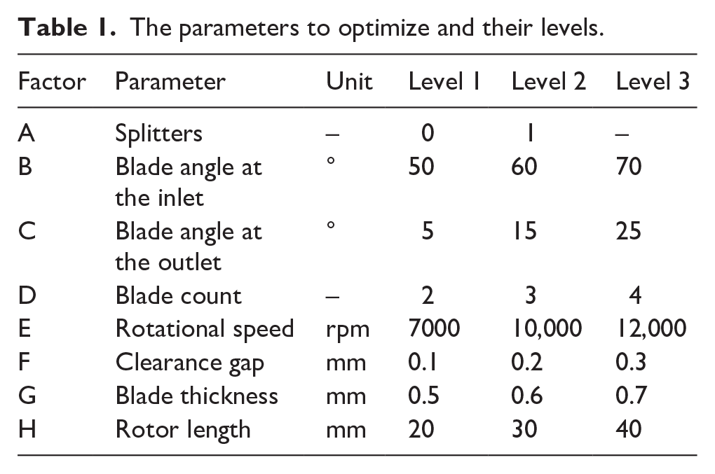
This study aimed to incorporate a wide range of design parameters. Rotors were designed with lengths varying from 20 to 40 mm and featured between two and four blades. The inlet blade angles ranged from 50° to 70°, while the outlet angles varied from 5° to 25°, and blade thicknesses were between 0.5 and 0.7 mm. Additionally, we developed models both with and without splitters. To avoid issues with crowding, the hub and shroud diameters were kept constant, while blade heights were adjusted using clearance gaps from 0.1 to 0.3 mm. The operating conditions included rotational speeds from 7000 to 12,000 rpm. The levels for each parameter are detailed in Table 1.

Table 1.

The parameters to optimize and their levels.

Factor	Parameter	Unit	Level 1	Level 2	Level 3
A	Splitters	–	0	1	–
B	Blade angle at the inlet	°	50	60	70
C	Blade angle at the outlet	°	5	15	25
D	Blade count	–	2	3	4
E	Rotational speed	rpm	7000	10,000	12,000
F	Clearance gap	mm	0.1	0.2	0.3
G	Blade thickness	mm	0.5	0.6	0.7
H	Rotor length	mm	20	30	40

Experimental design selection

To ensure the success of the experiment, a well-structured experimental design is essential. While methods like response surface design, full factorial design, and fractional factorial design are commonly used, they may not be suitable in constrained experimental spaces or when a linear model is inadequate. To address these limitations, we employed an optimal design approach that overcomes the constraints of traditional methods.

Optimal designs are defined as experimental designs that are optimal based on specific statistical criteria such as the average, determinant, eigenvalue, and variance. In this study, we utilized D-optimality, which relies on the determinant as a statistical criterion. The D-optimal design uses an iterative searching algorithm to minimize the covariance of parameter estimates, effectively maximizing the determinant of the design matrix.^7,8

The experimental design was generated using MATLAB code, which incorporated eight categorical parameters with three levels each, except for the first parameter, which had two levels. The code employed a quadratic regression model with a fixed number of runs and tries set at 50 and 1000, respectively. Table 2 presents the experimental design derived using the D-optimal method, along with the three output responses obtained from this design.

Table 2.

The D-optimal experimental design and the data collected from the CFD simulations.

RUN	Factors								Responses
RUN	A	B	C	D	E	F	G	H	PR (Pa)	TO (J)	EF (%)
1	0	60	15	2	12,000	0.2	0.7	20	29,854.2	0.00657813	30.0956
2	1	50	5	2	12,000	0.3	0.6	30	32,268.5	0.00774031	27.6471
3	1	70	5	4	10,000	0.3	0.7	40	13,404.5	0.00623032	17.1215
4	0	70	25	4	7000	0.2	0.5	20	2280	0.00282367	9.18447
5	1	60	25	2	10,000	0.2	0.6	40	22,032.5	0.00563108	31.1348
. . .	. . .	. . .	. . .	. . .	. . .	. . .	. . .	. . .	. . .	. . .	. . .
45	0	50	5	4	10,000	0.2	0.6	40	21,413.4	0.0065929	25.862
46	0	60	25	3	7000	0.2	0.7	40	7502.68	0.00312024	27.3525
47	1	50	15	2	7000	0.1	0.5	40	10,643.2	0.00375043	32.2667
48	0	70	5	4	10,000	0.3	0.6	20	14,005.8	0.00512299	21.7601
49	1	60	25	4	10,000	0.3	0.7	30	14,712	0.00506757	23.1017
50	1	60	15	3	12,000	0.2	0.5	20	29,025.9	0.00716505	26.8634

Computation fluid dynamic

Geometry

The device used in this study is the Model B presented previously in Bounouib et al.⁹ Following the original design, the device under investigation consists of four parts: an inducer, a rotor, a diffuser, and a straightener. The BladeGen tool integrated with ANSYS was used to create all components separately. According to the original design, a single version of the inducer, the diffuser, and the straightener were made. As for the rotor, according to the experimental design, 50 different versions were created.

Mesh

We employed the mesh configuration chosen after performing a mesh independence test for the meshing step. The mesh was generated using ANSYS TurboGrid. By combining the ATM-optimized topology and the Y⁺ method, we ensured a high concentration of elements in the areas near the walls where the pressure gradients are concentrated.

The result of this configuration is a mesh composed only of tetrahedral elements whose number varies from 4.5 × 10⁵ to 11.3 × 10⁵. These elements were mainly concentrated around the blades and at the blade tips.

CFD-pre settings

All simulations were carried out using ANSYS CFX. Generally, blood is known to be a non-Newtonian fluid with shear thinning properties. However, since the shear rates in VADs are typically greater than 100 s⁻¹, the assumption that blood is a Newtonian fluid is correct. Therefore, for blood properties, the density was set to 1050 kg/m³, and the dynamic viscosity was set to 0.0035 Pa s.¹⁰

For the boundary conditions, a 5 L/min flow rate was set at the inlet, and a 120 mmHg static pressure was placed at the outlet, defined as an opening. Since the flow velocity is null near the walls, a no-slip condition was used on the interior of the enclosure. The mixing plane method was used at the interfaces connecting the adjacent parts to obtain a flow similar to the actual flow. To predict turbulence in the flow, we used the two-equation eddy viscosity SST k–ω turbulence model, which was famous for its robustness and sensitivity.¹¹

Mathematical models

After all the simulations were conducted and all required data were extracted, we used another Matlab code to determine the parabola equation that best fit our data sets. The regression was executed using the data sets of the three outputs, namely pressure rise (PR), torque (TO), and hydraulic efficiency (FE). To find the equation that most accurately fits our data sets, we tested four different regression models (linear regression model, interactions regression model, pure quadratic regression model, and quadratic regression model) for each data set. To shorten the equations, we used a stepwise regression that eliminates all non-significant terms (p > 0.05).

Table 3 shows the results obtained after testing the four regression models on the three data sets. It can be seen that the quadratic model has the lowest squared error among all models, which signifies that with this model, the difference between predicted and observed values is the lowest. Furthermore, the quadratic model has the highest R² and adjusted R² values, indicating a good fit of the data to the regression model. Thus, the quadratic model was selected as a regression model.

Table 3.

Summary of the tested regression models.

Response	Model	p-value	R ²	R² adj	RMS error	Precision	Decision
DP	Linear	6.38 × 10⁻³¹	0.97	0.965	1.92 × 10³	Adequate
	Interactions	5.13 × 10⁻²⁵	0.984	0.976	1.58 × 10³	Adequate
	Pure quadratic	1.02 × 10⁻²⁶	0.989	0.984	1.31 × 10³	Adequate
	Quadratic	1.48 × 10⁻²²	0.995	0.991	9.95 × 10²	Adequate	Chosen
TO	Linear	5.73 × 10⁻³⁶	0.993	0.991	1.93 × 10⁻⁴	Adequate
	Interactions	5.73 × 10⁻³⁶	0.993	0.991	1.93 × 10⁻⁴	Adequate
	Pure quadratic	3.35 × 10⁻³⁷	0.994	0.992	1.78 × 10⁻⁴	Adequate
	Quadratic	7.59 × 10⁻²⁹	0.998	0.997	1.18 × 10⁻⁴	Adequate	Chosen
EF	Linear	7.21 × 10⁻¹¹	0.803	0.753	2.59	Inadequate
	Interactions	1.96 × 10⁻¹¹	0.927	0.876	1.84	Inadequate
	Pure quadratic	1.07 × 10⁻¹²	0.89	0.845	2.05	Inadequate
	Quadratic	3.8 × 10⁻¹²	0.942	0.898	1.66	Adequate	Chosen

The quadratic regression model selected for this study is formulated as follows:

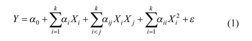
Y = α_{0} + \sum_{i = 1}^{k} α_{i} X_{i} + \sum_{i < j}^{k} α_{i j} X_{i} X_{j} + \sum_{i = 1}^{k} α_{i i} X_{i}^{2} + ε

(1)

Where Y is the predicted response, α₀ is the constant of the regression equation (the intercept). α_i, α_ij, and α_ii are the variables linear, interactions, and squared terms, respectively. X_i and X_j are the coded variables, k is the number of variables, and є is the model error.

After the general equation for the quadratic regression model is applied to the problem we are addressing, the equation for the quadratic regression model becomes as follows:

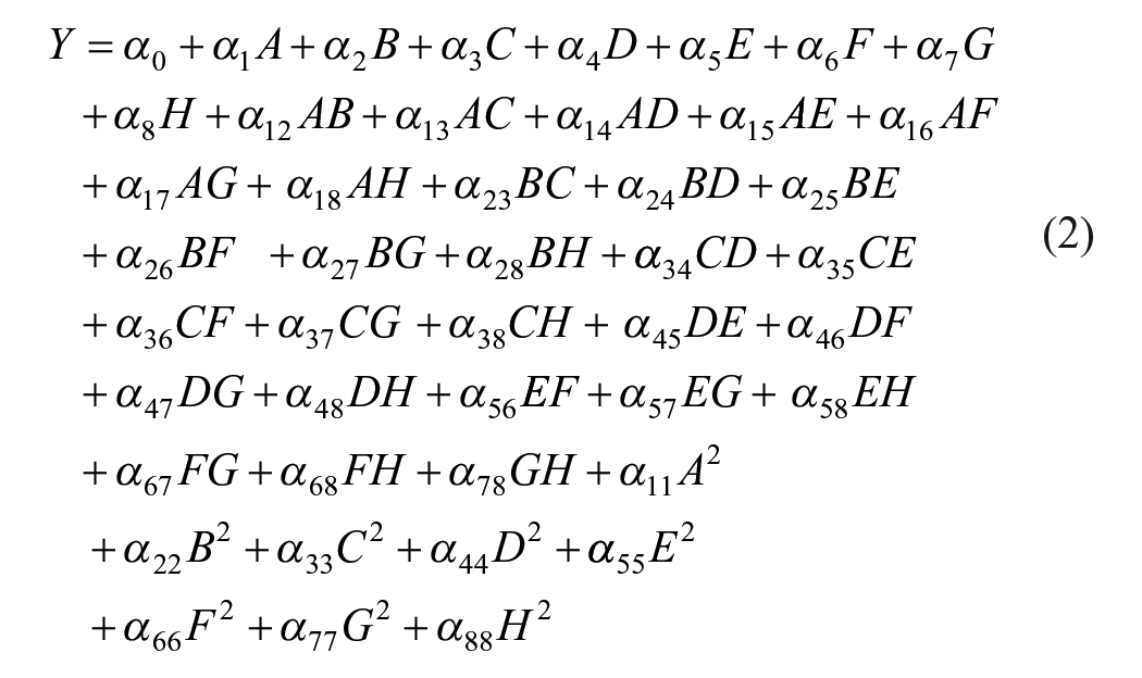
\begin{array}{l} Y = α_{0} + α_{1} A + α_{2} B + α_{3} C + α_{4} D + α_{5} E + α_{6} F + α_{7} G \\ + α_{8} H + α_{12} A B + α_{13} A C + α_{14} A D + α_{15} A E + α_{16} A F \\ + α_{17} A G + α_{18} A H + α_{23} B C + α_{24} B D + α_{25} B E \\ + α_{26} B F + α_{27} B G + α_{28} B H + α_{34} C D + α_{35} C E \\ + α_{36} C F + α_{37} C G + α_{38} C H + α_{45} D E + α_{46} D F \\ + α_{47} D G + α_{48} D H + α_{56} E F + α_{57} E G + α_{58} E H \\ + α_{67} F G + α_{68} F H + α_{78} G H + α_{11} A^{2} \\ + α_{22} B^{2} + α_{33} C^{2} + α_{44} D^{2} + α_{55} E^{2} \\ + α_{66} F^{2} + α_{77} G^{2} + α_{88} H^{2} \end{array}

(2)

After defining all variables and their associated terms for the three data sets, the characteristic equations for pressure rise (PR), torque (TO), and efficiency (EF) become as follows:

\begin{array}{l} D P = - 65, 950 - 10, 186 A + 1514.7 B - 326.73 C \\ + 11, 917 D - 2.2621 E + 26, 529 F + 77, 660 G \\ - 207.3 H + 162.59 A B - 98.602 B D + 82.974 C D \\ - 1074.9 C F + 8.3937 C H - 0.29217 D E \\ + 5642.9 D G - 87.314 D H - 5.3693 E F \\ + 4.3686 E G + 0.045064 E H - 61, 688 F G \\ - 12.307 B^{2} - 1018.5 D^{2} + 0.00026835 E^{2} \\ + 1.12 \times 10^{5} F^{2} - 1.02 \times 10^{5} G^{2} \end{array}

(3)

\begin{array}{l} T O = 0.014446 + 0.00027379 A - 0.00010337 B \\ - 7.00 \times 10^{- 5} C + 0.00061691 D - 3.45 \times 10^{- 7} E \\ - 0.0075603 F - 0.01763 G - 0.00020937 H \\ + 1.57 \times 10^{- 5} A B - 6.94 \times 10^{- 8} A E - 1.81 \times 10^{- 5} A H \\ + 0.00015709 B G + 1.25 \times 10^{- 5} C D - 6.13 \times 10^{- 9} C E \\ + 1.63 \times 10^{- 6} C H - 3.59 \times 10^{- 8} D E + 0.0010506 D F \\ - 4.06 \times 10^{- 7} E F + 2.94 \times 10^{- 7} E G + 1.48 \times 10^{- 8} E H \\ + 0.00016421 G H - 9.72 \times 10^{- 5} D^{2} + 4.99 \times 10^{- 11} E^{2} \\ + 0.010471 F^{2} \end{array}

(4)

\begin{array}{l} E F = 39.427 - 11.095 A + 0.7026 B \\ + 0.38561 C + 0.96616 D - 0.00078083 E \\ + 33.706 F - 46.85 G - 0.45514 H + 0.1532 A B \\ + 0.32516 A C - 1.2071 A D - 0.080426 B D \\ + 1.2731 B G + 0.025035 B H - 2.1894 C F \\ + 20.141 D G + 0.0047587 E F - 129.11 F G \\ - 1.9043 G H - 0.019259 B^{2} - 1.6241 D^{2} \end{array}

(5)

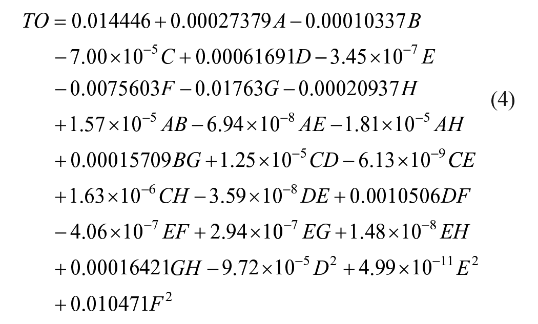
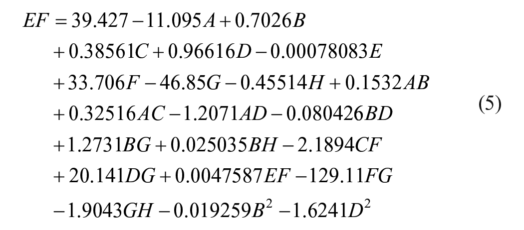
It should be noted that variables with a p-value above 0.05 were all removed.

Results

After fitting our data sets with the quadratic regression model, standard probability plots of the residuals from the fitted regression model were generated (Figure 1). These normal probability plots were used to validate the used regression model. From Figure 1, it can be seen that there are no aberrant values for the residuals, indicating that the observed values are highly correlated with the predicted values. Thus, it can be said that the selected regression model is highly reliable in determining the relationship between the eight input variables and the outcomes: pressure rise, torque, and efficiency.

Figure 1.

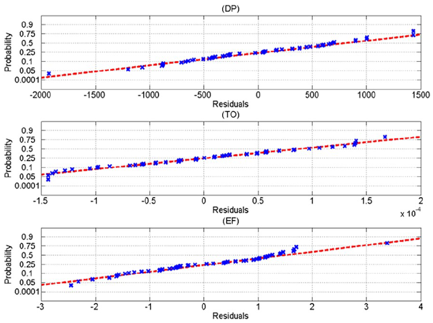
Normal probability versus residual.

Model validation

The validation of the mathematical model obtained by regression is essential in assessing the model’s credibility, as it shows the extent to which the predicted results correlate with the observed results. Therefore, to evaluate the adequacy of the mathematical models, the conditions outlined in the experimental design (Table 2) were used as inputs for the three mathematical models presented in equations (3–5). Subsequently, the observed results were compared to the predicted results. Analysis showed error rates between 0.1% and 24.85% for pressure rise, between 0.01% and 4.69% for torque, and between 0.19% and 21.08% for hydraulic efficiency.

To evaluate the effect of each parameter on the three outcomes, except for the parameter whose effect is being assessed, average values were used for each of the other parameters.

The influence of the design parameters on pressure rise

After analyzing the results, it was found that increasing parameters A, C, and F leads to a decrease in pressure rise, whereas increasing parameters E and H results in an increase in pressure rise. Conversely, the pressure rise follows a convex parabola with respect to parameters B, D, and G, reaching its peak when B = 56°, D = 3, and G = 0.6.

Figure 2 illustrates the response surface plots of pressure rise as a function of the interactions between different independent parameters. While previous findings indicated that pressure rise follows a convex parabola as B increases and decreases with increasing A, Figure 2(1) shows that at B = 70°, pressure rise increases with A. Similarly, although pressure rise generally decreases with increasing C and follows a convex parabola with increasing D, Figure 2(2) reveals that at D = 4, pressure rise increases with C. Figure 2(3) and 2(4) do not show any anomalies regarding the effects of E, F, G, and H on pressure rise.

Figure 2.

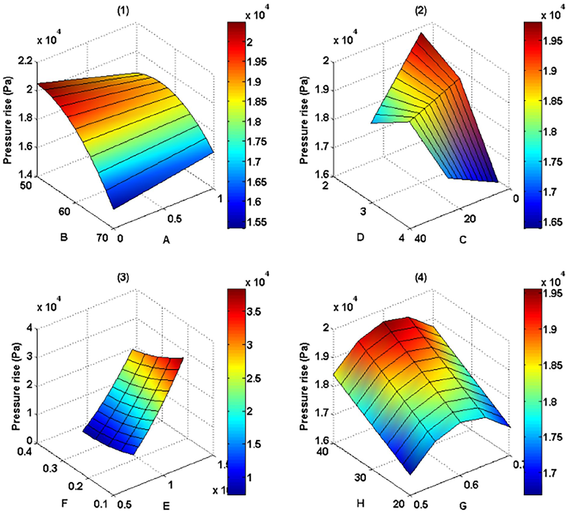
Response surface plots of the pressure rise as a function of the different interactions of the independent parameters.

The influence of the design parameters on torque

The analysis of the effect of the eight parameters on the torque required to drive the rotor revealed that increasing parameters A, E, and H leads to an increase in required torque. Conversely, increasing parameters B, C, F, and G results in a decrease in torque. The effect of parameter D on torque follows a convex parabola, with the maximum torque required at D = 3.

Although it was previously noted that increasing B decreases the torque and increasing A increases it, Figure 3(1) shows that at B = 50°, increasing A results in a decrease in torque. Figure 3(2) illustrates the interaction between parameters C and D on torque. While the impact of C remains as previously described, at C = 25°, the torque evolution does not follow a convex parabolic curve with increasing D, which is inconsistent with earlier findings. The interaction between parameters E and F, shown in Figure 3(3), does not exhibit any anomalies. Figure 3(4) demonstrates that the impact of H remains unchanged when interacting with G. However, it was found that G, which typically decreases torque, actually increases it when H exceeds 30 mm.

Figure 3.

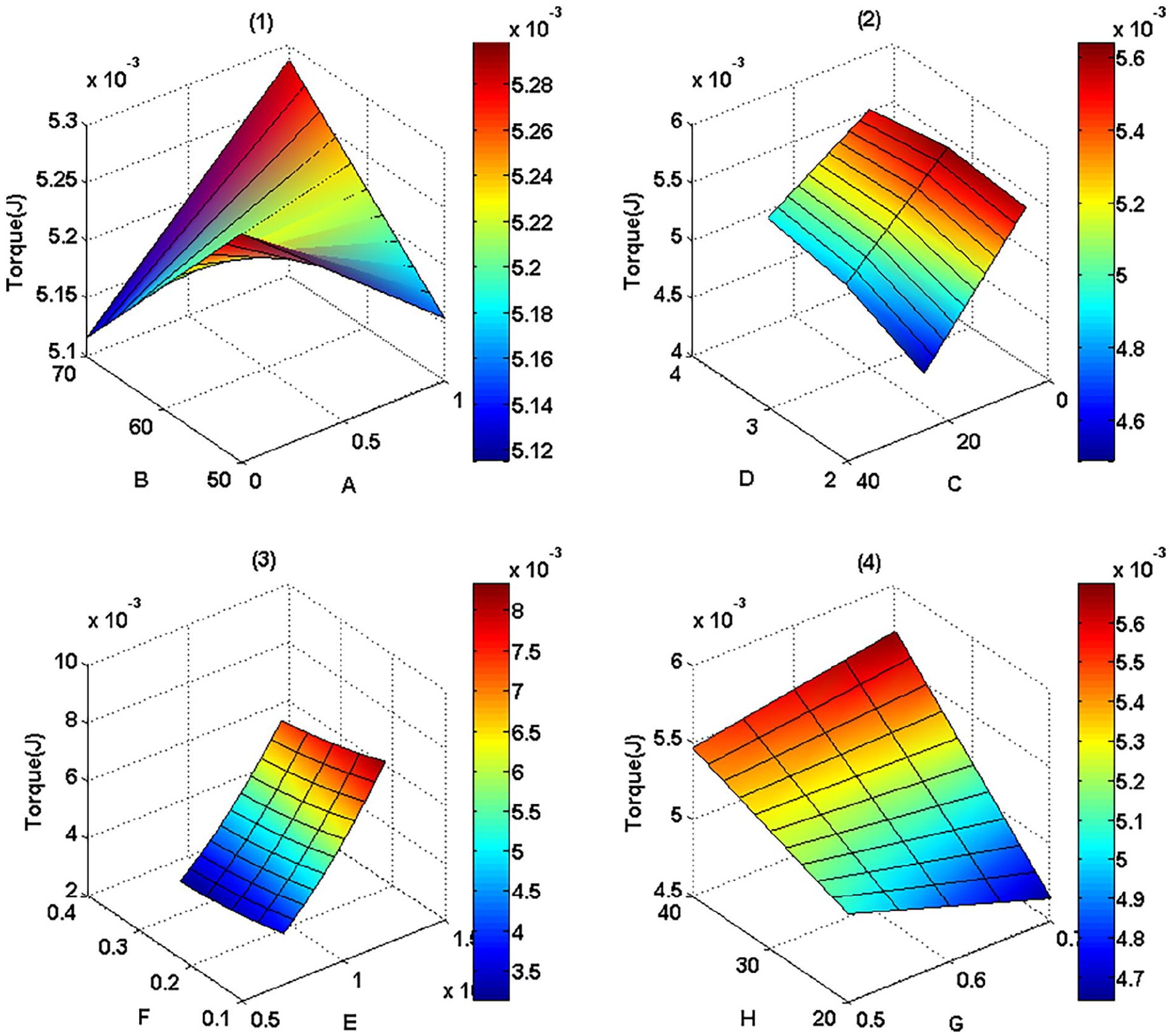
Response surface plots of the torque as a function of the different interactions of the independent parameters.

The influence of the design parameters on hydraulic efficiency

The analysis of the effects of all selected parameters on the hydraulic efficiency of the pump showed that increasing parameters A, D, F, and H led to a decrease in efficiency, while increasing parameters C, E, and G resulted in an increase. The effect of parameter B on hydraulic efficiency followed a convex parabolic pattern, with maximum efficiency reached at B = 55°.

Figure 4 illustrates the evolution of hydraulic efficiency under various parameter interactions. As previously noted, hydraulic efficiency follows a convex parabola with increasing B and decreases with increasing A. However, Figure 4(1) shows that at B = 70°, hydraulic efficiency increases with A. Figure 4(2) confirms that the effects of parameters C and D remain consistent with earlier findings, showing no abnormal efficiency patterns. Although parameter E generally increases efficiency, Figure 4(3) indicates that at F = 0.1 mm, efficiency decreases with increasing E. It was noted that G increases efficiency while H decreases it, but Figure 4(4) reveals that the effect of G is reversed at H = 40 mm, and the impact of H is reversed when G is less than 0.6 mm.

Figure 4.

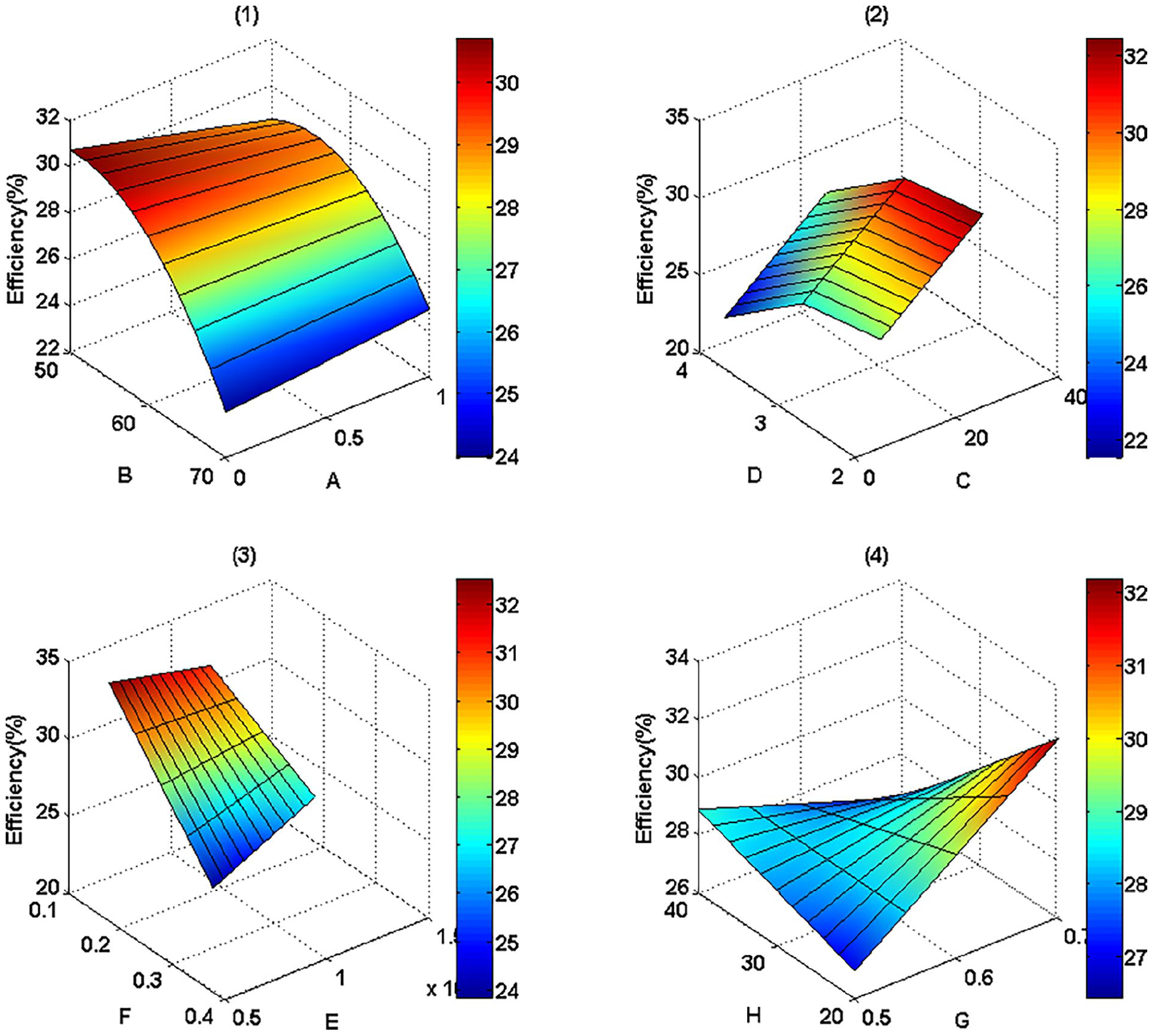
Response surface plots of the hydraulic efficiency as a function of the different interactions of the independent parameters.

Optimal conditions

This paper aims to identify optimal design parameters and operating conditions that satisfy the predetermined objectives of maximizing the pump’s pressure rise and hydraulic efficiency while minimizing the torque required to drive the rotor. To determine the maximum pressure rise achievable, a range of values for the eight parameters was tested using equation (3). The highest pressure rise found was approximately 44,352.98 Pa (≈332.67 mmHg), achieved with A = 0 (no splitters), B = 50°, C = 25°, D = 3, E = 12,000 rpm, F = 0.1 mm, G = 0.7 mm, and H = 40 mm.

Similarly, equation (4) was used to find the minimum torque required to drive the rotor, which was approximately 15 × 10^–4 J. This value was obtained with A = 0 (no splitters), B = 50°, C = 25°, D = 2, E = 7000 rpm, F = 0.3 mm, G = 0.7 mm, and H = 20 mm. All possible combinations of the specified parameters were also tested using equation (5) to predict the maximum obtainable hydraulic efficiency. The highest efficiency found was about 43.48%, achieved with A = 1 (with splitters), B = 52°, C = 25°, D = 3, E = 7000 rpm, F = 0.1 mm, G = 0.7 mm, and H = 20 mm.

All results were validated through CFD simulations.

Discussion

The main objective of this study was to identify the optimal design parameters and operating conditions that maximize pressure rise and hydraulic efficiency while minimizing the torque required to drive the rotor. The eight parameters selected for this study were splitters, inlet blade angle, outlet blade angle, blade count, rotational speed, clearance gap, blade thickness, and rotor length.

By setting all parameters to intermediate values and varying one parameter at a time, we obtained an overview of each parameter's effect on the three outcomes:

- Parameter A (Splitters): Adding splitters decreased pressure rise, likely because they increase flow velocity in the latter part of the rotor, reducing pressure. Splitters also increased torque due to the additional load on the motor from the extra blades. Consequently, hydraulic efficiency decreased due to the combined effect of reduced pressure rise and increased torque.

- Parameter B (Inlet Blade Angle): Increasing the inlet blade angle caused pressure rise to follow a convex parabola. A steeper blade angle pushes more fluid into the rotor, increasing outlet pressure. However, if the angle is too steep, fluid flow into the rotor decreases, causing a pressure drop at the outlet. Torque also increased with blade angle due to the higher load from the increased flow rate.

- Parameter C (Outlet Blade Angle): A larger outlet blade angle decreased pressure rise, likely due to increased flow velocity. Higher flow velocity smoothens the flow, reducing the load on the blades and thus decreasing torque. The resulting increase in hydraulic efficiency likely stems from the torque reduction outweighing the decrease in pressure rise.

- Parameter D (Blade Count): Pressure rise and torque followed a convex parabolic curve as blade count increased. More blades push more fluid and increase motor load, but when blade count becomes too high, the smaller inlet passages restrict fluid entry, reducing pressure rise and torque. Hydraulic efficiency decreased due to the more significant drop in pressure rise compared to the reduction in torque.

- Parameter E (Rotational Speed): Higher rotational speed increased the number of revolutions per minute, pushing more fluid out and raising both pressure rise and torque. Since the increase in pressure rise was greater than the torque increase, hydraulic efficiency improved.

- Parameter F (Clearance Gap): Increasing the clearance gap decreased pressure rise, torque, and hydraulic efficiency. A larger gap reduces blade height, pushing less fluid and lowering pressure rise. The reduced blade height also lowers motor load, decreasing torque. The efficiency drop was due to the pressure rise reduction being more significant than the torque decrease.

- Parameter G (Blade Thickness): Thicker blades decreased the volume of fluid per passage, reducing pressure rise and torque. However, hydraulic efficiency increased because the torque reduction was more significant than the pressure rise decrease.

- Parameter H (Rotor Length): Increasing rotor length increased blade length, pushing more fluid out and raising both pressure rise and torque. The increase in torque was more substantial than the pressure rise, leading to a decrease in hydraulic efficiency.

Conclusion

This paper aims to find the optimal design parameters for a VAD rotor under development. The parameters that were selected and investigated in this study are splitters (with/without), inlet blade angle (50°–70°), outlet blade angle (5°–25°), blade count (2–4), rotational speed (7000–12,000 rpm)), clearance gap (0.1–0.3 mm), blade thickness (0.5–0.7 mm), and rotor length (20–40 mm). The objective is to find the optimal values for each parameter to obtain maximum pressure increase, maximum hydraulic efficiency, and minimum torque.

The experimental design was constructed using the D-optimal method with the number of runs set to 50 and the number of tries set to 1000. Once all simulations were run according to the experimental design, the pressure rise, torque, and hydraulic efficiency obtained in each simulation were retained.

After testing several regression models, the quadratic regression model was chosen because it has the highest R², the highest adjusted R², and the lowest RMS error. Using the specified regression model, three equations (3–5) related to pressure rise, torque, and efficiency were obtained. The obtained mathematical models were validated by studying the correlation between the experimental and predicted results.

After testing various combinations of parameters using the obtained mathematical models, we determined the varieties that met the predefined conditions. For example, in terms of pressure rise, we found that its highest value was about 44,352.98 Pa, the highest value of hydraulic efficiency was approximately 43.48%, while in terms of torque, its lowest value was about 15 × 10⁻⁴ J.

Footnotes

Declaration of conflicting interests

The author(s) declared no potential conflicts of interest with respect to the research, authorship, and/or publication of this article.

Funding

The author(s) received no financial support for the research, authorship, and/or publication of this article.

ORCID iD

Mohamed Bounouib

References

Anderson

Wood

Allaire

, et al. Numerical studies of blood shear and washing in a continuous flow ventricular assist device. ASAIO J 2000; 46: 486–494.

Bounouib

Es-Sadek

Taha-Janan

, et al. Numerical study of an impeller design for a new ventricular assist device. MATEC Web Conf 2019; 286: 07017.

Geerts

. Experimental and numerical study of an axial flow pump. PhD Thesis (2006), 252.

Song

Chua

Lim

TM.

Numerical study of a bio-centrifugal blood pump with straight impeller blade profiles. Artif Organs 2010; 34: 98–104.

Chua

Lim

, et al. Numerical simulation of an axial blood pump. Artif Organs 2007; 31: 560–570.

Throckmorton

Untaroiu

CFD analysis of a mag-lev ventricular assist device for infants and children: fourth generation design. ASAIO J 2008; 54: 423–431.

Isksioui

Ennima

Bourekkadi

, et al. The use of intelligent systems and innovation to model and optimize fused deposition modeling process parameters for time manufacturing and material consumption. J Theor Appl Inf Technol 2020; 98: 11.

Smucker

Krzywinski

Altman

Optimal experimental design. Nat Methods 2018; 15: 559–560.

Bounouib

Benakrach

Es-Sadek Zeriab

, et al. Numerical study of a new ventricular assist device. Artif Organs 2020; 44: 604–610.

10.

Curtas

Wood

Allaire

, et al. Computational fluid dynamics modeling of impeller designs for the HeartQuest left ventricular assist device: ASAIO J 2002; 48: 552–561.

11.

Menter

Kuntz

Langtry

Ten years of industrial experience with the SST turbulence model. Heat Mass Transf 2003; 4(1): 625–632.