Breaking the Chain: How Arrests Reduce the Probability of Near Repeat Crimes

Abstract

Objectives:

Near repeat patterns have been identified for a host of different crimes, but effective strategies to reduce near repeats have had more variable results. This study identifies near repeat crime patterns in Dallas, TX, and examines the effects of an arrest on reducing the probability of future crime.

Method:

Using open-source crime data from the Dallas Police Department from July 2014 through June 2018, we identified near repeat patterns for shootings, interpersonal robberies, residential burglaries, and thefts from motor vehicles. Logistic regression models were used to test the effect of an arrest on reducing near repeat crimes; controls for geographic, demographic, and temporal factors were included in each model.

Results:

Near repeat calculations suggest violent crime clustered closely in time and space, with property crime dispersed over larger spatial and temporal dimensions. Across all four crime types, findings suggest arrests resulted in 20%–40% reductions in a near repeat follow-up crime.

Conclusions:

In line with past research on shootings, arrests reduced the likelihood of subsequent crimes. This suggests policing strategies to increase arrests may be a fruitful way to reduce near repeat crime patterns.

Keywords

near repeat arrests spatial analysis crime analysis

Near repeat crime patterns are the concentration of crime incidents in both space and time (Townsley et al., 2003). Drawing from epidemiology, the idea is that the occurrence of a crime creates a heightened risk of a subsequent crime in nearby areas (e.g., a street block or two) for a short time (e.g., a few days to weeks; Knox, 1964). In sum, near repeat crime patterns are a well-established criminological finding for many different crime types (S. D. Johnson et al., 2007; Ratcliffe & Rengert, 2008; Youstin et al., 2011). But, studies evaluating policing strategies to address near repeat crime patterns have shown mixed results (Elffers et al., 2018; Groff & Taniguchi, 2019; R. B. Santos & Santos, 2016; Stokes & Clare, 2019). Here, we focus on whether arresting individuals reduces the probability of a near repeat crime.

We build on prior work in two particular ways. Prior analyses of shooting data have established that arrests reduce the probability of near repeat patterns (Wyant et al., 2012). In this work, we establish whether this relationship also holds true for not only shootings in another sample but also for three instrumental crimes: residential burglaries, interpersonal robberies, and thefts from motor vehicles. If near repeat patterns are largely a function of the same individuals committing multiple offenses in a short spree (S. D. Johnson et al., 2009), it may be the incapacitation or deterrent effects of an arrest are larger for instrumental crimes than for shootings, which are theoretically driven by retaliatory violence (Loftin, 1986; Ratcliffe & Rengert, 2008).

Given that macro-level evidence of the effectiveness of arrests in reducing future crime are more equivocal (Bursik et al., 1990; Chamlin et al., 1992; Levitt, 1998), examining very small space and time windows provides a more direct test of the efficacy of arrest-based strategies that are less influenced by potential endogeneity problems. If arrests provide subsequent reductions in near repeat offending, it can provide the foundation for assessing the benefits of increasing arrest rates in reference to reduced crime rates.

Second, a variety of more recent work has established different predictive factors that correlate with the probability of a near repeat crime (Garnier et al., 2018; Moreto et al., 2014; Piza & Carter, 2018). In addition to formulating a regression model incorporating these demographic and facility factors to account for additional confounds not present in prior work, we include a factor for the historical density of crimes. Given that hot spots of crime tend to be temporally stable (Curman et al., 2014; Weisburd et al., 2004; Wheeler et al., 2016), not accounting for the underlying density can result in confounds in predicting which crimes are likely to result in a near repeat offense.

A large sample of 4 years of open data on crime incidents and arrests from Dallas, TX, was used for this study. Compared to prior work on shootings, we find that arrests tended to have similar effectiveness in reducing the probability of a near repeat offense for all the crimes types examined (Wyant et al., 2012), typically ranging from a reduction of 20%–40% near repeats across different space and time windows. Given the low arrest rates for many of the crime types under study, prioritizing events that have a higher probability of a near repeat crime may be a reasonable strategy for police departments to tackle near repeat crimes.

Literature Review

Overview of Near Repeat Crime Patterns

Near repeat crime patterns occur when two or more crimes occur in a short spatial–temporal window (Townsley et al., 2003). The basic idea is that a crime incident, often called the originator/initiator event, spurs one or more subsequent crime incidents, often called the near repeat events, in the immediate spatial area and in a short time frame of the originator event. The premise is adapted from epidemiology and the transmission of infectious diseases (Knox, 1964). For example, an originator house is burglarized on a Monday, and the next-door neighbor becomes a near repeat house when it is burglarized the following Wednesday. While most work on near repeat crime patterns has been focused on burglary (S. D. Johnson et al., 2007; Townsley et al., 2003), it has been shown to extend to a variety of different crime types: robbery, shootings, theft from motor vehicles, thefts of motor vehicles, arson, assault, economic crimes, piracy, and terroristic events (Behlendorf et al., 2012; Block & Fujita, 2013; Braithwaite & Johnson, 2012; Haberman & Ratcliffe, 2012; Lockwood, 2012; Marchione & Johnson, 2013; Powell et al., 2019; Sturup et al., 2018; Townsley et al., 2008; Turchan et al., 2019; Wells et al., 2012; Youstin et al., 2011; Zhang et al., 2015).

Two hypotheses have long been proposed to explain repeat and then ultimately near repeat crime patterns: (1) risk heterogeneity (or the flag hypothesis) and (2) state dependence (or the boost hypothesis; Farrell & Pease, 1993; Short et al., 2009). Risk heterogeneity is simply the hypothesis that certain characteristics lead to higher overall propensity for crime victimization in some areas (e.g., see Bowers & Johnson, 2005; Pitcher & Johnson, 2011). In effect, targets/places with greater propensity for crime will be crime hot spots (Weisburd, 2015). It follows that near repeat patterns will occur simply by chance due to crimes being more common in those hot spots (see S. D. Johnson, 2008; Pitcher & Johnson, 2011). For example, if a street segment tends to have an average of 10 robberies per year, and those robberies are distributed according to a Poisson distribution, the probability of a near repeat crime happening within a week on that same street segment is over 17% (Park & Eck, 2013). In sum, the more crime in a small area, the greater the probability of crime occurring close in space and time when observations are made in shorter, fixed windows (S. D. Johnson, 2008; Pitcher & Johnson, 2011).

The second potential explanation of near repeat patterns is state dependence or boost hypothesis. State dependence occurs when the risk of crime over time is not constant but increases due to a previous victimization. A shooting can increase the risk of a future shooting due to retaliatory violence (Loftin, 1986; Ratcliffe & Rengert, 2008). A burglary can increase the risk of a future burglary because a burglar learned an effective way to enter similarly built homes in an area (Bowers & Johnson, 2004). Another example is that the same offender can victimize multiple targets within a short spree (e.g., stealing from many open cars in the same parking lot in a short time period) or in a more serial nature (e.g., burglarizing a new house every day of the week; Wheeler, 2016). In the former case, offenders are restricted to a short spatial window due to not being able to travel far in a particular time period (Ratcliffe, 2006). The latter can potentially be within a larger spatial area, but due to offenders’ limited awareness space of potential victimizable targets (Brantingham & Brantingham, 1993), they often forage in a smaller, known area for potential victims (Jacobs, 2010).¹ Several studies have confirmed (using arrest data) that near repeat crimes are more likely to have been committed by the same offender (Bernasco, 2008; Davies & Marchione, 2015; D. Johnson, 2013; S. D. Johnson et al., 2009). One study even found that the probability of a near repeat in space and time is higher for networked offenders, suggesting that offenders may vicariously share information on potential targets (Lantz & Ruback, 2017).

Recently, researchers have attempted to identify the spatial characteristics that predict whether a crime is likely to result in a near repeat. Broadly, these involve either identifying micro-place characteristics of the built environment (Garnier et al., 2018; Moreto et al., 2014; Piza & Carter, 2018) or neighborhood demographic characteristics (Bowers & Johnson, 2005; S. D. Johnson et al., 1997; Nobles et al., 2016).

Studies that focus on micro-places tend to measure nearby facilities and land uses that increase the probability of a near repeat event. For just one example of a facility, both Moreto et al. (2014) and Garnier et al. (2018) examined whether places nearby pawnshops increased the chance of a near repeat burglary or robbery victimization (respectively) in Newark, NJ. Findings from both studies of Newark, NJ, suggested the concentration of high-risk micro-locations provided the necessary criminogenic environment needed to sustain crime hot spots (Moreto et al., 2014), and hot spots were the result of aggregate clusters of local interactions resulting from individuals congregating and being attracted to favorable locations and one another (Garnier et al., 2018). Piza and Carter (2018) examined burglary and motor vehicle thefts in Indianapolis and classified crimes into either isolated events, initiator events (those that precipitate a near-repeat, sometimes also referred to as an originator event), or near repeat event. The researchers identified near repeat victimization patterns for residential burglary and motor vehicle theft, with near repeat motor vehicle thefts expanding farther out from each initial incident than residential burglaries (Piza & Carter, 2018). They then used multinomial models based on local land-use factors and five neighborhood measures of social disorganization to identify whether those characteristics are more likely to predict initiator events. Piza and Carter (2018) found concentrated disadvantage, population density, and racial heterogeneity were consistently associated with initiator and near repeat burglary and motor vehicle theft, but geographic mobility and young male population effects varied across crime types.

Studies that examine greater neighborhood characteristics often find that areas with higher levels of concentrated disadvantage have more near repeats (Bowers & Johnson, 2005; S. D. Johnson et al., 1997; Nobles et al., 2016). While this makes sense, in that those areas also tend to be higher crime, others have found wide spatial variations in near repeats (Groff & Taniguchi, 2018, 2019), or that near repeat patterns spatially shift over time (S. D. Johnson & Bowers, 2004). One additional explanation for more near repeats in disadvantaged neighborhoods (beyond they are typically higher crime) is that individuals in low-income areas lack the capital to fund physical security measures (Bowers & Johnson, 2005; S. D. Johnson et al., 1997; Nobles et al., 2016).

Understanding spatial variations in near repeat risk can help identify efficient strategies to allocate resources to mitigate future risk. Contrary to one’s intuition, Chainey et al. (2018) find that most near repeats occur outside of hot spots, and so police strategies to address near repeats are not as simple as chasing the dots on the map following a crime that may result in a near repeat event (also see Haberman & Ratcliffe, 2012). This pattern likely occurs because although near repeats are more likely to occur within hot spots, the majority of crimes are not themselves within hot spots (under most definitions of hot spots, Groff & Taniguchi, 2019).

Crime Prevention Based on Near Repeats

Crime prevention undertaken by policing agencies in response to near repeat patterns can be broadly classified under three types: (1) victim-focused strategies (i.e., target hardening), (2) proactive policing strategies (e.g., more patrols in the area of the near repeat crimes), and (3) arrest-based strategies.

First, victim-focused strategies have been applied toward preventing near repeat burglary victimization. Such interventions have included publicly funded target-hardening installations (Hirschfield et al., 2010), contacting the victims of burglary and providing informational pamphlets to them and neighbors (Stokes & Clare, 2019), and conducting security audits to reduce the likelihood of a future residential burglary (Groff & Taniguchi, 2019). Target-hardening approaches can focus on area-based characteristics or at-risk targets, but Hirschfield et al. (2010) suggest a combined approach. Hirschfield et al. (2010) and Stokes and Clare (2019) find publicly funded prevention investments were not cost-effective solutions, and repeat burglary risk did not decrease in the respective studies. Results from Groff and Taniguchi’s (2019) study also indicate no significant difference between control and treatment zones where a target-hardening strategy was implemented. Operation Swordfish, a police-led intervention in Birmingham, UK, combined target hardening (by increasing appearance of capable guardianship) with informing neighbors of vulnerabilities local burglars had taken advantage of so they might be able to address security within their own homes (S. D. Johnson et al., 2017). Considered a low-intensity but highly focused implementation, Operation Swordfish was found to result in a statistically significant reduction in risk for neighbors of burgled homes. However, S. D. Johnson et al. (2017) caution the effect of the intervention was small in magnitude, and the rest of their analyses suggested nonstatistically significant differences between treatment and control zones.

Second, proactive policing strategies are those that devote extra patrol resources in response to near repeat events. Fielding and Jones (2012) find that deploying extra patrols in Trafford, England, in response to near repeat burglaries over an extended period of time resulted in a 27% reduction of burglaries over a 12-month period. Although not specifically focused on responding to near repeat patterns, Wells and Wu (2011) do not find evidence that a specialized gun crime unit in Houston reduced near repeat shootings. In a predictive policing study of proactive patrol (in which targeted locations are both based on historical patterns and elevated risk due to near repeats), Mohler et al. (2015) find slight reductions in overall crime. Elffers et al.’s (2018) examination of foot patrols in the area surrounding a recent burglary location found no difference in burglary crime rates after comparing the treatment and control groups. Finally, Santos and Santos published a series of articles using data collected by the Port St. Lucie Police Department on proactive policing in microtime hot spots. Microtime hot spots were meant to target potential near repeat patterns. Four studies demonstrated the effectiveness of directed police patrols in reducing residential burglaries and thefts from motor vehicles (R. B. Santos & Santos, 2016). Immediate, directed patrol and increases in police response reduced residential burglaries and thefts from motor vehicles in microtime hot spots (R. B. Santos & Santos, 2015; R. G. Santos & Santos, 2015a, 2015b).

Third, two studies have examined the impact of arrest strategies on subsequent gun crimes (Wu & Wells, 2016; Wyant et al., 2012). In a study of over 5,000 firearm arrests and shootings in Philadelphia, Wyant et al. (2012) demonstrated using a modified bivariate Knox test that following an arrest, firearm shootings within 800 ft and 4 days were lowered by about 28%. In a replication study in Houston, Wu and Wells (2016) find more mixed results, although they do detect fewer shootings than expected at 400 ft and 4 days after the arrest.

Given the mixed results of victimization and proactive policing strategies, reducing near repeat victimization via arrests may be a fruitful approach. There are two theoretical mechanisms through which arrests can subsequently reduce future offending: (1) deterrence and (2) specific incapacitation. Arrests are hypothesized to decrease crime by signaling to would-be offenders that the risk of apprehension is high (Sampson & Cohen, 1988; Wilson & Boland, 1978). In short, offenders may observe an arrest and increase their risk perceptions or hear about an arrest from others (Lantz & Ruback, 2017; Parker & Grasmick, 1979; Stafford & Warr, 1993; Wyant et al., 2012).

Alternatively, offenders who are arrested and subsequently incarcerated will be specifically incapacitated as they will not have the capability to commit another offense. Even if offenders are then subsequently released within a short window (such as on bail), presumably their internal estimate of the probability of being caught in the future should be increased (Anwar & Loughran, 2011; Piquero et al., 2011). If near repeat victimization is driven by high-risk offenders repeatedly committing crimes, then arrests should be particularly effective at reducing the likelihood of a near repeat incident.

Although past analyses of firearm arrests and shootings have shown fleeting effects, shootings are one type of near repeat pattern that is not theoretically explained by the same offender committing multiple offenses in a short time period but by retaliatory violence. So, it seems likely that specific deterrence or incapacitation due to an arrest is likely to have a much larger effect reducing near repeats for instrumental crimes such as burglaries, robberies, and thefts from motor vehicles. Thus, this analysis extends prior work examining the micro-spatial patterns of shootings and firearm arrests to examine the impact of arrests on near repeat patterns of more crime types.

Based on this prior literature, we subsequently test two hypotheses in this work:

Hypothesis 1: An arrest will reduce the probability of a near repeat burglaries, robberies, shootings, and thefts from motor vehicles.

Hypothesis 2: An arrest will reduce the probability of a near repeat shooting but will have a smaller effect compared to instrumental crimes.

Data and Methods

Data

Dallas, TX, is the study site. Data for the analysis were collated from several different open sources. First, crime incident and arrest data from July 2014 through June 2018 were provided by the Dallas Police Department. The specific crime types included were shootings, interpersonal robberies, residential burglaries, and thefts from motor vehicles. These data include already geocoded data at the address level. Second, data for control variables capturing the locations of potentially criminogenic facilities and land use were taken from different open data sources such as the street index database (Cortright & Mahmoudi, 2016), Dallas County parcel data, and commercial databases such as LexisNexis and Reference USA. Third, sociodemographic control variables were developed using the 2017 5-year American Community Survey estimates at the block-group level.

Dependent Variable

Recall the present study tests if arrests reduce the probability of a near repeat crime incident in the future. The dependent variable is a dichotomous measure of whether or not a subsequent crime incident occurs within a specific spatial–temporal window of each crime. For every crime event, we conduct a search of whether a future crime occurred within a particular distance and time threshold and label that a “1.” All crimes that did not result in a near repeat were then coded “0.” So, instead of the approach in Piza and Carter (2018) which classifies crimes into isolates, initiator, or near repeat crimes, here each crime incident is a unit of analysis and has the potential to be an initiator event. This is a key because recent research has demonstrated that an incident that is a near repeat may itself later spawn additional near repeat incidents (i.e., near repeat chains; see Haberman & Ratcliffe, 2012), which is accounted for in the present approach. For simplicity in the main analysis, we focus on identifying near repeat crime events within 1,000 ft and 7 days. This is based on past research on typical sizes of near repeat patterns, along with our estimates of significant near repeats in this sample tend to always be significant among the different crime types given that window. But, given selecting space–time thresholds is arbitrary (Ratcliffe & Rengert, 2008), sensitivity analyses examining the deterrent effect of an arrest over different time and space thresholds are also shown.²

Independent Variables

The main independent variable of interest in this analysis is whether a crime event resulted in an arrest. Events that are recorded as having an arrest are then coded as a “1,” and events without an associated arrest are coded as a “0” in the subsequently regression models. We do not count case clearances via other means (e.g., “exceptional clearance”), and only those cases specifically mentioning an arrest occurred are coded as “1.” This is because the theoretical mechanism of specific deterrence and/or incapacitation is specific to the actual arrest act.

Statistics for the number of crimes and the proportion of near repeats within 1,000 ft and 7 days are broken down by whether an arrest occurred and are included in Table 1. From this, one can surmise that arrests have a small effect, around a 10% reduction in near repeat crimes for shootings and interpersonal robberies and a 20% reduction for burglaries. However, thefts from motor vehicles increase slightly. Arrest rates for each crime type vary inversely with their severity and frequency; shootings have the highest overall arrest rate (26%), followed by robberies (12%), burglaries (4%), and thefts from motor vehicles (3%).

Table 1.

Descriptive Statistics for Different Crime Types.

Crime Type	No Arrest		Arrest
Crime Type	Total N	Future Crime (%)	Total N	Future Crime (%)
Shooting	2,948	5.2	1,048	4.7
Interpersonal robbery	10,206	14.0	1,351	12.7
Residential burglary	25,157	20.6	983	16.1
Theft from motor vehicles	55,354	27.7	1,531	30.7

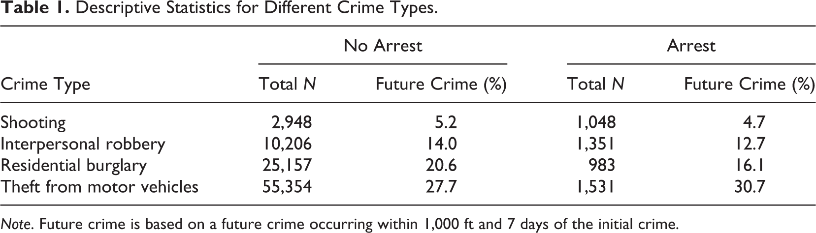
Note. Future crime is based on a future crime occurring within 1,000 ft and 7 days of the initial crime.

As previously mentioned, the probability of a near repeat is greatly influenced by the baseline density at which the crime occurs (S. D. Johnson, 2008; Pitcher & Johnson, 2011; Park & Eck, 2013). More simply, long-term hot spots could have more near repeats because as the number of crimes increases in a micro-area, the probability that crimes will be close in time increases. As such, it is important to take this prior crime density factor into account. To do this, we use historical crime data that were provided directly by the Dallas Police Department from 2010 through June 30, 2014, to measure the historical crime density for each specific crime type. We use historical data to prevent the measure from being endogenous with the near repeat outcome measure, which is examined using data from July 1, 2014, through June 30, 2018. Given that hot spots of crime tend to be quite temporally stable over time (Andresen et al., 2017; Curman et al., 2014; Weisburd et al., 2004; Wheeler et al., 2016), these historical measures are suitable to control for that historical crime density, while providing a measure that is not endogenous with the current crime data being predicted (i.e., not using future crime density to predict historical near repeats).

For a simplified example of our analysis, say a theft from a motor vehicle occurred at the coordinates [0,0] on January 1, 2016, and we are interested in examining near repeats within 7 days and 1,000 ft. If another theft from a motor vehicle occurred at coordinates [100,100] on January 4, 2016, we would classify that origin event as having a near repeat “1” for the outcome. Additionally, if an arrest did not occur for that origin event, it would receive “0” for the arrest indicator. As some places have many more crimes than others, we also include a term of all thefts from motor vehicles that occurred within 1,000 ft of the [0,0] coordinate in the historical crime data (from January 1, 2010, through June 30, 2014). To illustrate how this would potentially impact the results, imagine two scenarios: one in which there were a total of 50 crimes within 1,000 ft of [0,0] in the historical data, versus 300 crimes within 1,000 ft in the historical data, which equal a density of approximately 0.2 and 1.3 crimes on a per 7-day basis, respectively. For the lower density estimate under a Poisson process, it would be expected to have a near repeat crime 20% of the time within 7 days simply by chance. Whereas for the higher density estimate, it would be expected to have a near repeat 73% of the time.³

Because the prior crime density can have such a large impact on the resulting probabilities of a near repeat crime, it is not only important to include as a potential covariate in the analysis, but we also examine its interaction with whether an arrest reduces the probability of a near repeat crime. In areas that have a very low probability of a near repeat, it may be that arrests are not as effective in preventing a future crime (a floor effect). It also may be the case in areas where crimes are very common (so have a very high probability of a near repeat), arrests additionally do not appear to be effective (a ceiling effect). The latter may especially be the case if a place is very heterogeneous in who commits a crime there, and so many near repeats are not a function of the same offender(s) committing multiple crimes. The ability to model different effects in a regression framework is one reason we use a regression modeling approach, as opposed to the modified Knox test approach as used in Wyant et al. (2012).

Next, given prior work showing that near repeat patterns are influenced by different facilities, we have included these additional factors into our model (Garnier et al., 2018; Moreto et al., 2014; Piza & Carter, 2018). We include a total of 18 different crime generator factors. Each of these crime generators is encoded as distance from a crime to the nearest crime generator. Given these are control variables and are not the main interest of the analysis, we do not spend substantial time examining these factors in the subsequent models. Wheeler and Steenbeek (2020) provide a more detailed description of the data sources and how they are relevant in predicting microlevel crime patterns, which similarly extends to predicting near repeat crime patterns (Garnier et al., 2018; Piza & Carter, 2018). These particular crime generator factors include commercial establishments: (1) large business retailers (e.g., Walmart, The Home Depot, CVS), (2) smaller food and clothing stores, (3) gasoline stations, (4) eating and drinking places, (5) liquor stores, (6) large entertainment areas (e.g., movie theaters, concert halls), (7) smaller entertainment areas (e.g., gyms, bowling alleys) and hair salons, (8) motels, (9) hotels, (10) shopping malls, (11) banks, and (12) check cashing stores. We also included noncommercial land-use factors of (13) libraries, (14) middle and high schools, (15) public railway stations (Dallas Area Rapid Transit [DART] stations), (16) apartment complexes, (17) hospitals, and (18) mobile home parks.

We also include a set of covariates based on the residential census demographics, again similar to that in Piza and Carter (2018). These measures are taken from the 2017 5-year American Community Survey estimates. These measures include the following: (1) the percentage of families in poverty, (2) the percentage of individuals unemployed (of those over 16 and in the workforce), (3) the percentage of individuals receiving some type of government assistance, (4) the percentage of female-headed households with children under 18, (5) the percentage of the population that is Hispanic, (6) the percentage of the population that is Asian, (7) the percentage of the total population that is non-Hispanic Black, (8) the percentage of families that have moved in the prior year, and (9) the total number of the population under 17. These are similar to measures that have been used in prior near repeat analyses (Piza & Carter, 2018; Ratcliffe et al., 2016) and represent typically well-established factors that proxy social disorganization theories of crime (Pratt & Cullen, 2005; Sampson et al., 1997; Shaw & McKay, 1969). These demographic characteristics are assigned based on the block group the originator event resided in.

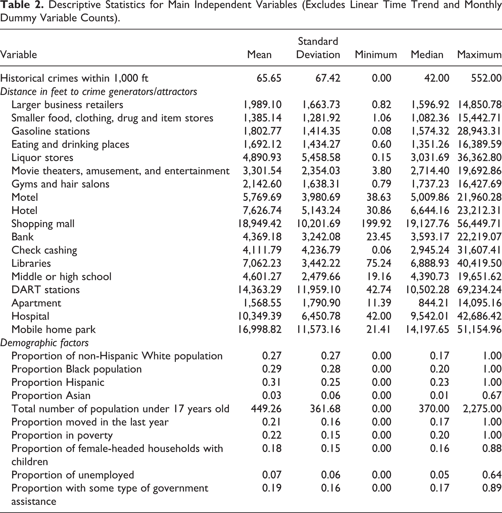
The final set of factors are temporal controls. We include a set of dummy variables for the month of the incident and a linear time trend (as crimes have overall been slightly decreasing in Dallas over the examined period). These should take into account potential seasonal or overall time trend effects, which may result in particular periods having a higher or lower probability of a near repeat crime in space and time (Piza & Carter, 2018). Table 2 provides descriptive statistics for the variables used in the analysis, aggregated across each crime type.

Table 2.

Descriptive Statistics for Main Independent Variables (Excludes Linear Time Trend and Monthly Dummy Variable Counts).

Variable	Mean	Standard Deviation	Minimum	Median	Maximum
Historical crimes within 1,000 ft	65.65	67.42	0.00	42.00	552.00
Distance in feet to crime generators/attractors
Larger business retailers	1,989.10	1,663.73	0.82	1,596.92	14,850.78
Smaller food, clothing, drug and item stores	1,385.14	1,281.92	1.06	1,082.36	15,442.71
Gasoline stations	1,802.77	1,414.35	0.08	1,574.32	28,943.31
Eating and drinking places	1,692.12	1,434.27	0.60	1,351.26	16,389.59
Liquor stores	4,890.93	5,458.58	0.15	3,031.69	36,362.80
Movie theaters, amusement, and entertainment	3,301.54	2,354.03	3.80	2,714.40	19,692.86
Gyms and hair salons	2,142.60	1,638.31	0.79	1,737.23	16,427.69
Motel	5,769.69	3,980.69	38.63	5,009.86	21,960.28
Hotel	7,626.74	5,143.24	30.86	6,644.16	23,212.31
Shopping mall	18,949.42	10,201.69	199.92	19,127.76	56,449.71
Bank	4,369.18	3,242.08	23.45	3,593.17	22,219.07
Check cashing	4,111.79	4,236.79	0.06	2,945.24	31,607.41
Libraries	7,062.23	3,442.22	75.24	6,888.93	40,419.50
Middle or high school	4,601.27	2,479.66	19.16	4,390.73	19,651.62
DART stations	14,363.29	11,959.10	42.74	10,502.28	69,234.24
Apartment	1,568.55	1,790.90	11.39	844.21	14,095.16
Hospital	10,349.39	6,450.78	42.00	9,542.01	42,686.42
Mobile home park	16,998.82	11,573.16	21.41	14,197.65	51,154.96
Demographic factors
Proportion of non-Hispanic White population	0.27	0.27	0.00	0.17	1.00
Proportion Black population	0.29	0.28	0.00	0.20	1.00
Proportion Hispanic	0.31	0.25	0.00	0.23	1.00
Proportion Asian	0.03	0.06	0.00	0.01	0.67
Total number of population under 17 years old	449.26	361.68	0.00	370.00	2,275.00
Proportion moved in the last year	0.21	0.16	0.00	0.17	1.00
Proportion in poverty	0.22	0.15	0.00	0.20	1.00
Proportion of female-headed households with children	0.18	0.15	0.00	0.16	0.88
Proportion of unemployed	0.07	0.06	0.00	0.05	0.64
Proportion with some type of government assistance	0.19	0.16	0.00	0.17	0.89

Methods

To test whether an arrest results in a reduced probability of a near repeat event, we use logistic regression analysis (for an overview, see Hilbe, 2009). In this model, we include whether the current crime resulted in an arrest, the prior crime density per week (based on the same threshold distance for crimes occurring from 2010 through June 2014), an interaction between the two, the remaining crime generator, and demographic and temporal control variables as have been used in prior research. The logistic regression model can then be formally written as:

Prob [Future Crime < f (d, t)] = {logit}^{- 1} [β_{0} + β_{1} (Arrest) + β_{2} (Prior Crime Density) + β_{3} (Arrest \cdot Prior Crime Density) + {Σβ}_{k} X_{k}],

where we predict the probability that a future crime occurs within a threshold distance d and time t. Hypothesis 1 is that $β_{1}$ , the coefficient for whether an arrest occurred, is negative and so reduces the probability of a near repeat. Given that we also estimate an interaction between arrests and prior crime density (i.e., arrests may be more or less effective in high-crime areas), we assess this effect using marginal effect estimates over the domain of prior crime densities, holding all other variables at their means (Mize, 2019). The remaining control variables are then represented as $β_{k} X_{k}$ .

This model is estimated for individual crime types of thefts from motor vehicles, interpersonal robberies, residential burglaries, and shootings. Hypothesis 2 is that while we expect that the arrest effect for shooting incidents is negative (Wyant et al., 2012), it is closer in absolute magnitude toward zero than the other instrumental crimes.

Results

Near Repeat Analysis

Knox ratios and accompanying p values for each of the four crime types were generated for 30 spatial bins (100 ft each) and 30 temporal bins (1 day each), using 99 permutations to assess statistical randomness (Ratcliffe & Rengert, 2008) in the results (Tables listed in Online Appendix B due to their size). Results from the near repeat calculations suggest the day after an instigator event carries the highest risk for a repeat or near repeat event for each of the four crime types, but overall patterns in time and space deviate between crime types. Shootings were found to cluster closely in time and space, with the highest level of risk for a repeat shooting occurring on the 1st day and within 300 ft of the instigator incident. Near repeat interpersonal robberies showed a larger spatial and temporal distribution than shootings, with an increased risk to the surrounding area (0–300, 500–700, 1,900–2,200, 2,400–2,700 ft) during the day after a robbery. The risk to the 3,000 ft around the initial robbery decreases as time passes. This is true for residential burglaries and thefts from motor vehicles but to a lesser extent.

For a month after a burglary or vehicle break-in, the offense location carries a higher risk of near repeat offenses. Up to a week after the initiator event, near repeat burglaries and vehicle break-ins follow the pattern of a series of crimes occurring closer to the initial offense location within the week and then spreading in distance as time continues. These findings are consistent with prior research finding near repeat patterns are more likely than by chance and that those patterns fade for further spatial and time distances, but it is difficult to make specific rules for how far away in space or time near repeat patterns are likely to occur across crime types.

Regression Model Results

Table 3 displays the results of logistic regression models predicting the likelihood of a future crime for each crime type based on a series of spatial, temporal, and population characteristics, the historical crime density (number of crimes per week from January 1, 2010, to June 30, 2014), and whether there was an arrest for each offense. The tables are limited to coefficients for arrests and prior crime density. Online Appendix A contains a full set of the coefficients for all models.

Table 3.

Logistic Regression Model Predicting Whether a Future Crime Occurs within 1,000 Ft and 7 Days Across Different Crime Types.

	Coefficient	Standard Error	p Value	Low OR	High OR
Interpersonal robbery
Arrest	−0.24	0.14	0.09	−0.53	0.04
Crime density	4.13	0.25	0.00	3.64	4.62
Arrest × Crime Density	0.95	0.59	0.10	−0.20	2.10
Theft from motor vehicles
Arrest	0.13	0.10	0.19	−0.06	0.31
Crime density	1.95	0.04	0.00	1.87	2.04
Arrest × Crime Density	−0.25	0.17	0.13	−0.58	0.08
Residential burglary
Arrest	−0.03	−0.27	0.79	−0.27	0.21
Crime density	1.46	24.79	0.00	1.34	1.57
Arrest × Crime Density	−0.50	−1.83	0.07	−1.04	0.04
Shooting
Arrest	−0.17	0.26	0.51	−0.67	0.33
Crime Density	9.68	1.78	0.00	6.19	13.16
Arrest × Crime Density	0.72	2.51	0.77	−4.20	5.64

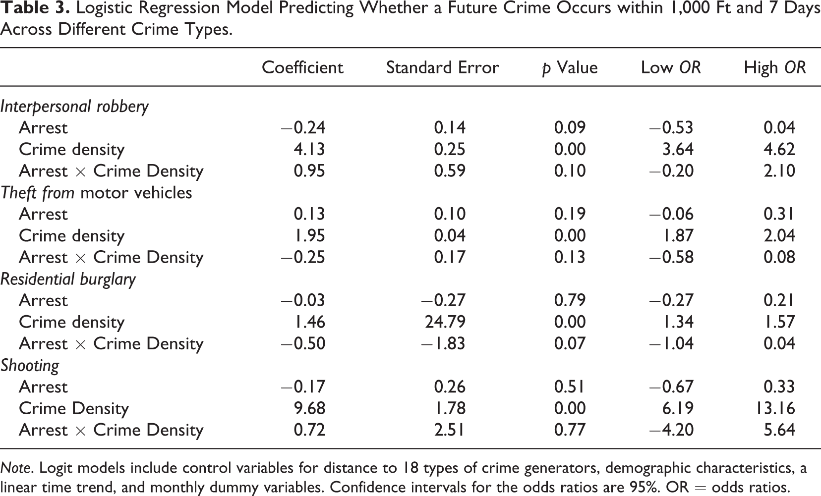
Note. Logit models include control variables for distance to 18 types of crime generators, demographic characteristics, a linear time trend, and monthly dummy variables. Confidence intervals for the odds ratios are 95%. OR = odds ratios.

The presence of an arrest reduces the likelihood of future interpersonal robberies (at p value .09), but all other direct effects of arrests across the crime types are not statistically significant. Considering the interaction effects, as the historical crime density increases, the effect of an arrest gets smaller for both thefts from motor vehicles and burglaries, although the p values for those interaction effects are above .05. This provides evidence that arrests have a larger deterrent effect in high-crime areas for those two crimes. The interaction effects for robberies and shootings are positive, suggesting that arrests have a larger deterrent effect in low-crime areas but again have p values above .05. Overall, these results suggest that arrests have little impact on the probability of a near repeat event, but we graph the estimated reduction in the probability of arrest conditional on the historical crime density, as the interaction effects are difficult to intuitively understand.

Each of the following four figures contains two graphs; the left-hand side of Figures 1 –4 illustrates the effect of historical crime density on the probability of a future crime depending on the presence of an arrest, holding all other control variables at their means, for each of the crime types under examination. The right-hand side graph shows a confidence interval of the difference between those two predicted probability lines and a pairwise 95% confidence interval of that difference in probabilities.

Figure 1.

The left-hand graph displays the predicted probabilities of a future near repeat robbery (within 1,000 ft and 7 days) from initial event, for events with and without an arrest, given different historical crime densities per 7 days (within 1,000 ft); the right-hand graph displays the estimated difference between those two probabilities with a 95% confidence interval of the difference.

Figure 2.

The left-hand graph displays the predicted probabilities of a future near repeat burglary (within 1,000 ft and 7 days) from initial event, for events with and without an arrest, given different historical crime densities per 7 days (within 1,000 ft); the right-hand graph displays the estimated difference between those two probabilities with a 95% confidence interval of the difference.

Figure 3.

The left-hand graph displays the predicted probabilities of a future near repeat shooting (within 1,000 ft and 7 days) from initial event, for events with and without an arrest, given different historical crime densities per 7 days (within 1,000 ft); the right-hand graph displays the estimated difference between those two probabilities with a 95% confidence interval of the difference.

Figure 4.

The left-hand graph displays the predicted probabilities of a future near repeat theft from motor vehicle (within 1,000 ft and 7 days) from initial event, for events with and without an arrest, given different historical crime densities per 7 days (within 1,000 ft); the right-hand graph displays the estimated difference between those two probabilities with a 95% confidence interval of the difference.

In Figure 1, showing the probability of a future robbery within 1,000 ft and 7 days, one can see arrests decrease the probability of a future crime at low historical crime densities and then predict a higher probability of future offenses and higher historical crime densities. Examining the difference between these probabilities shows that the confidence interval of the difference in those probabilities covers 0 for the entire line. Figure 2 for burglaries appears to be more promising—even though each individual coefficient was not statistically significant at the .05 level, the predicted reduction in future burglaries appears to be much larger when taking into account the interaction effect. At areas with the highest historical crime density in the data, an arrest results in over a 20% reduction in a future near repeat burglary occurring. Figure 3 (shootings) shows very little difference in the estimated predictions. Thefts from motor vehicles (Figure 4) show reductions in higher crime areas, but the confidence interval of the difference tends to always cover 0.

The prior analysis focused on the crime reduction effects, given a specific distance and time threshold, 1,000 ft and 7 days specifically. Given that these thresholds are arbitrary, we have conducted additional analyses to examine the crime reduction effect of arrests at the distance thresholds of 500–3,000 ft (in increments of 500 ft) as well as the time thresholds of 3, 7, 14, 21, and 28 days. Note these are cumulative thresholds, and so, an event with a near repeat in 500 ft and 3 days will also count as a near repeat within 2,000 ft and 14 days. We fit the same models as previously, controlling for the characteristics of the built environment, demographic factors, and the prior crime density (within the corresponding distance buffer). While we also include the interaction effect of the arrest and prior crime density in these models (same as before), here we focus on the direct effects of arrests for simplicity.

Figure 5 plots the linear coefficient of the effect that an arrest has on the probability of a future crime, illustrating the varying effects over different distance (the x-axis) and day (different lines) near repeat events for each crime type under examination. For ease in interpretation, standard errors are not included on the chart, but coefficients with a p value of less than .05 have an additional point superimposed on the line. The general patterns for each crime type show that larger temporal bands (gray to green) tend to show greater crime reduction effects, and the shorter temporal bands of 3 and 7 days (brown) tend to hover close to the null of zero crime reductions. Robberies at shorter distances of 500–1,500 ft tend to show the largest crime reductions, but for the other crime types, larger distances of 2,000–3,000 ft tend to have the largest reductions in near repeats. The main analysis examining the near repeat reduction effects at 7 days and 1,000 ft then appear to be conservative estimates across all of the different crime types.

Figure 5.

Coefficient for arrest effect, given different distance and time thresholds for examining near repeats. Note. Coefficients that had a p value of less than .05 are given a dot.

Thefts from motor vehicles actually show a statistically significant increase in the probability of a near repeat at the shortest distance and time interval examined (500 ft and 3 days). A potential explanation for this is that the current analysis does not take into account the timing of when the arrest occurred (that is not available in the open data set), and so, multiple events in a short period (e.g., someone breaking into five different cars in the same parking lot over a short time period in a single spree) will result in a near repeat event, but one that is unactionable from the police departments perspective (Groff & Taniguchi, 2018). If those runs of many crimes are more likely to result in increased police scrutiny and a subsequent higher probability of an arrest, our estimate of the reduction of near repeat events outside of the initial string will be biased upward. To account for this given the data that are accessible, like Groff and Taniguchi (2019), we eliminate near repeat events that occur within 24 hr of the initial event and rerun the same analyses. Those results are displayed in Figure 6.

Figure 6.

Coefficient for arrest effect, only including future crimes that occurred at least 24 hr after the initiator crime event, given different distance and time thresholds for examining near repeats. Note. Coefficients that had a p value of less than .05 are given a dot.

The results when eliminating near repeat events within 24 hr of the initiating event generally show that arrests have a larger effect of reducing the probability of a near repeat crime. The exception to this is burglaries, which show near equivalent patterns to the original results. Robberies now show the strongest effects at 3 or 7 days and 1,500 ft but have similar effects at larger time bins and shorter distance bins. Thefts from motor vehicles tend to again show greater deterrent effects at larger distance and temporal bins, as do shootings. Of those statistically significant effects, they tend to hover in between coefficients of −.2 and −.5 for all crime types, which when exponentiated correspond to odds ratios of .82 and .61, respectively. This suggests a fairly consistent estimate of the reduction of a near repeat crime on the magnitude of 20%–40% following an arrest, albeit at varying distance and temporal thresholds for each crime type examined here.

In reference to Hypothesis 2, that shootings will have a smaller near repeat reduction following an arrest, this does not appear to be the case for any of these analyses at varying distance and time thresholds. Consistent with the prior analysis focusing on 1,000 ft and 7 days, if anything there is weak evidence that arrests following a shooting result in a larger reduction of a near repeat event than the other instrumental crime types examined. Given the size of the standard errors, conducting an actual test of the differences in coefficients, the contrasts would rarely show a statistically significant difference between the effects for different crime types over the majority of the different space and time thresholds. Thus, there is no evidence here that arrests for instrumental crimes result in larger reductions of near repeat crimes than shootings.

Discussion

To summarize the findings, we find mixed evidence of the reduction in near repeat crimes following an arrest across different instrumental and expressive crime types. While the space and time distances at which reductions were observed varied across the different crime types, in total, the largest reductions tended to be around 20%–40% for each crime type. This replicates the findings of prior work only examining shootings and arrests by Wyant et al. (2012), who found in Philadelphia that an arrest reduced the probability of a near repeat crime by approximately 30%–50%. Unlike the findings in Wyant et al. (2012) though, the space–time distance of those effects were observed at larger distance and temporal bins across the crime types, more frequently at 2,000 ft and 21 days or more, compared to only around 1,000 ft and a few days for Wyant et al. (2012). This is also counter to the findings in Wu and Wells (2016), who only find evidence of a deterrent effect on shootings for arrests in a smaller space–time window.

In reference to the importance of the findings toward theory, prior evaluations of macro- and neighborhood-level patterns of arrests and subsequent crime declines have tended to produce mixed findings (Bursik et al., 1990; Chamlin et al., 1992; Levitt, 1998). Examining the reduction in near repeat crimes provides a way to show a relationship between arrests and subsequent crime in a more precise way than is possible when examining aggregate-level statistics. It is still the case that one cannot identify the difference between specific incapacitation as opposed to general deterrent effects with this limited administrative data, but given that we know many crimes are committed by a few individuals (Ratcliffe & Kikuchi, 2019), focusing on solving near repeat crimes seems a fruitful tactic for police departments to attempt to improve on.

Unlike hypothesized, we do not find evidence that the arrest effect is larger for instrumental crimes relative to an arrest for shootings. This is an important finding that not only replicates prior findings for the deterrent effect of arrests following shootings (Wyant et al., 2012) but provides evidence that solving violent crimes results in a lower probability of retaliation (Leovy, 2015). Improving clearance rates for serious violence is not impossible (Braga & Dusseault, 2018) and is also expected to have downstream effects of improving perceptions of police as well (Braga et al., 2019). These estimates of crime reductions can potentially be used to justify increased detective resources, especially given the costs associated with serious violence (Hunt et al., 2019). Beyond policing, it is possible that community outreach violence interrupters also reduce the probability of retaliatory violence (Butts et al., 2015), and their effectiveness could be determined in a similar manner to the analysis we have conducted here.

The same rationale could be applied to devoting more investigatory resources toward solving instrumental crimes of theft from motor vehicles and burglary, but those crimes tend to have a much lower cost to the police (Hunt et al., 2019). As prior work suggests police departments already take quite seriously shootings and near repeat robberies (Haberman & Ratcliffe, 2012; Wyant, 2014), it may be the case that other cost-effective strategies will be needed to improve arrest rates to prevent near repeat crimes. Technological solutions can be potentially used to increase arrest clearances such as closed-circuit television (Piza et al., 2014; Ratcliffe et al., 2019) or street lighting (Chalfin et al., 2019). It may be feasible to move such (mobile) cameras or lights in response to an emerging chain of near repeats, as opposed to relying on permanent locations for either.

It may also be the case that police can differentially devote resources to cases that have a higher probability of a near repeat offense. One way to do this is to identify cases in which there is a higher probability of a near repeat crime (Garnier et al., 2018; Moreto et al., 2014; Piza & Carter, 2018) and then devote more detective resources to those events (or prevent them from being triaged). Another may be to use other automated detection processes to identify whether a particular crime is linked to other crimes (Chohlas-Wood & Levine, 2019; Porter, 2016). Again, those criminal events within a linked chain should then get higher priority from detectives, as those individuals have established a prior history that suggests they will commit a future crime.

The findings that arrests reduce near repeats within the range of 20%–40% should also be taken in light of evidence of the mixed findings of target-hardening approaches (Groff & Taniguchi, 2019; Stokes & Clare, 2019). It is also true that traditional police responses, such as increased patrol or street stops, may be a mechanism for police to reduce near repeat crime events (R. B. Santos & Santos, 2016; R. G. Santos & Santos, 2015b; Wooditch & Weisburd, 2016). While individuals typically have positive perceptions of police undertaking such target-hardening responses to burglaries (Antrobus & Pilotto, 2016; Groff & Taniguchi, 2019), the lack of consistent evidence showing crime reduction effects undermines their overall utility. It may be those resources are better spent on general patrol or detective resources to solve crimes.

The findings should be interpreted in light of several limitations for the analysis. A major limitation of the work is that this is an observational research design. It is possible that arrests are confounded with other factors that explain their correlation with subsequent reductions in near repeat crimes. One example in which this could occur would be whether less professional individuals are more likely to be arrested following a crime, and those same individuals are also less likely to commit another crime in the near future. This would result in a bias that concludes arrests have a larger deterrent effect on near repeat crimes than they do in reality. We attempt to take into account potential biases by including covariates for the historical crime density at places as well as a host of other crime generator and demographic characteristics (Piza & Carter, 2018). But absent an experiment or stronger quasi-experimental design, this will always be a threat to the validity of the findings.

The bias could work the other way as well, in that if an individual commits multiple crimes in a short period, those strings of crimes are likely to gather more police attention (Haberman & Ratcliffe, 2012) and subsequently have a higher rate of being solved. So, arrests are associated with more crimes in the short term. This is partially solved in the analysis by only counting near repeats that occur 24 hr post the initial event (Groff & Taniguchi, 2018), and the evidence indicates this bias occurs for robberies, thefts from motor vehicles, and shootings, given the results, but not for burglaries. Future work could distinguish between the exact temporal timing of arrests associated with the criminal event. Only particular configurations of near repeats in which associated events are outside of a certain range are actionable from a police department’s perspective (Davies & Marchione, 2015).

Given we do not have timing information associated with arrests in this data set, an additional biasing factor is that an arrest may occur after a near repeat crime has occurred in our analysis. This would bias the effect of an arrest on subsequent near repeats toward zero, and so, our findings demonstrating potential effects of 20%–40% may potentially be underestimates due to this bias. We believe this is not a fatal flaw however, as given the low clearance rates for these events, many are never assigned a detective, and so, the majority of arrests only occur where an individual is caught in the act. This is especially true for thefts from motor vehicles in Dallas, and given the overall estimates are quite similar across crime types, we believe this signals that the results are not dramatically biased.

The second limitation is that given the unknown potential space–time window of where we should observe a deterrent effect conditional on arrest, we test the deterrent effect with different space and time thresholds. While here this illustrates that larger deterrent effects are seen at larger space–time windows, it also brings up the possibility that multiple comparisons are a reasonable explanation for the findings. Despite the large sample sizes, tests of crime reductions tended to only show a statistically significant crime reduction effect by a small margin. One potential way to account for this in future research is to estimate the decay effect directly, such as by decomposing the offspring effect in a Hawkes model into two components, crimes with and without arrests (Achab et al., 2018; Mohler et al., 2018; Reinhart & Greenhouse, 2018).

The findings here will ultimately need to be tested in the field to prove their worth. As such, future research should focus on experimental or quasi-experimental designs that attempt to improve arrest rates following crimes. Identifying cases that have a higher probability of resulting in a near repeat offense and devoting more investigative resources is one way in which that can be accomplished (Garnier et al., 2018). Another is identifying chains of near repeats and increasing investigative resources in response (Haberman & Ratcliffe, 2012). In either case, the results here are promising that such initiatives have potential to reduce near repeat crimes.

In reference to reproducibility of the results, we have provided replication materials. This includes the original data sources collated from open sources, as well as python, Stata, and SPSS scripts used to conduct the near-repeat analysis, prepare the data, generate regression models, and graph the results. The Dallas Police Department has provided one of the most comprehensive open sources of crime data among police agencies in the world (Ackerman & Rossmo, 2015; Wheeler et al., 2017), allowing us the ability to conduct this analysis. But, it also identifies one particular weakness in the data as well—the inability to match the time stamp of the occurrence of an arrest to when the crime occurred. It is likely the case that open data sources provided by police departments will always need to undergo periodic revision to incorporate more information to better the analytic potential of the data.

For example, much analysis of the arrest and crime relationship relies on either aggregate Uniform Crime Reporting (UCR) data (Chamlin et al., 1992), or microlevel National Incident Based Reporting System (NIBRS) data sources (Roberts, 2007). But both of these data sources lack specific microlevel geographic identifiers (such as census tract or addresses of the events), which preclude replicating the near repeat analysis we conduct. If however NIBRS were to incorporate address-level information, it would be possible to conduct a widespread analysis of the microlevel deterrence effects of arrests on near repeat crimes across many police jurisdictions. That would allow much broader generalizability of the results and not be dependent on idiosyncratic open data sources or special relationships between academics and police departments. Although academic and police practitioner relationships are no doubt a good thing (for both police and academics), limiting the ability to conduct analysis of key policing processes to the privileged few is not.

That being said, currently both for academics and police departments, there are little to no incentives to provide open data and reproducible code. Police departments have some slight incentives such as assistance from governmental bodies (or negative conditions for funding conditional on reporting). As academics, we have zero incentives to share our code for this article. We do so simply because that is a necessary step to ensure the integrity of scientific research. Relying on the goodwill of researchers to share replication materials has the same obvious disadvantage that allowing police departments to pick and choose what data to disseminate—it can be capricious. What a better system to incentivize openness may look like we are not sure, but both academics and police will no doubt need to make strides in this area to be more professional and rigorous.

Supplemental Material

Supplemental Material, sj-pdf-1-cjr-10.1177_0734016821999707 - Breaking the Chain: How Arrests Reduce the Probability of Near Repeat Crimes

Supplemental Material, sj-pdf-1-cjr-10.1177_0734016821999707 for Breaking the Chain: How Arrests Reduce the Probability of Near Repeat Crimes by Andrew P. Wheeler, Jordan R. Riddell and Cory P. Haberman in Criminal Justice Review

Footnotes

Authors’ Note

Data and code to replicate the findings can be obtained from https://www.dropbox.com/sh/ 72 q i 7 wm 60 ndqve/AABgFB 8 zwGHG 6 xjExvaD 01 EGa?dl= 0

Declaration of Conflicting Interests

The authors declared no potential conflicts of interest with respect to the research, authorship, and/or publication of this article.

Funding

The authors received no financial support for the research, authorship, and/or publication of this article.

Supplemental Material

The supplemental material for this article is available online.

Notes

References

Achab

Bacry

Gaïffas

Mastromatteo

Muzy

J. F.

(2018). Uncovering causality from multivariate Hawkes integrated cumulants. Journal of Machine Learning Research, 18(192), 1–28.

Ackerman

J. M.

Rossmo

D. K.

(2015). How far to travel? A multilevel analysis of the residence-to-crime distance. Journal of Quantitative Criminology, 31(2), 237–262.

Andresen

M. A.

Curman

A. S.

Linning

S. J.

(2017). The trajectories of crime at places: Understanding the patterns of disaggregated crime types. Journal of Quantitative Criminology, 33(3), 427–449.

Antrobus

Pilotto

(2016). Improving forensic responses to residential burglaries: Results of a randomized controlled field trial. Journal of Experimental Criminology, 12(3), 319–345.

Anwar

Loughran

T. A.

(2011). Testing a Bayesian learning theory of deterrence among serious juvenile offenders. Criminology, 49(3), 667–698.

Behlendorf

LaFree

Legault

(2012). Microcycles of violence: Evidence from terrorist attacks by ETA and the FMLN. Journal of Quantitative Criminology, 28(1), 49–75.

Bernasco

(2008). Them again? Same-offender involvement in repeat and near repeat burglaries. European Journal of Criminology, 5(4), 411–431.

Block

Fujita

(2013). Patterns of near repeat temporary and permanent motor vehicle thefts. Crime Prevention and Community Safety, 15(2), 151–167.

Bowers

K. J.

Johnson

S. D.

(2004). Who commits near repeats? A test of the boost explanation. Western Criminology Review, 5(3), 12–24.

10.

Bowers

K. J.

Johnson

S. D.

(2005). Domestic burglary repeats and space-time clusters: The dimensions of risk. European Journal of Criminology, 2(1), 67–92.

11.

Braga

A. A.

Brunson

R. K.

Drakulich

K. M.

(2019). Race, place, and effective policing. Annual Review of Sociology, 45, 535–555.

12.

Braga

A. A.

Dusseault

(2018). Can homicide detectives improve homicide clearance rates? Crime & Delinquency, 64(3), 288–315.

13.

Braithwaite

Johnson

S. D.

(2012). Space-time modeling of insurgency and counterinsurgency in Iraq. Journal of Quantitative Criminology, 28(1), 31–48.

14.

Brantingham

P. L.

Brantingham

P. J.

(1993). Nodes, paths, and edges: Considerations on the complexity of crime and the physical environment. Journal of Environmental Psychology, 13(1), 3–28.

15.

Bursik

R. J.

Grasmick

H. G.

Chamlin

M. B.

(1990). The effect of longitudinal arrest patterns on the development of robbery trends at the neighborhood level. Criminology, 28(3), 431–450.

16.

Butts

J. A.

Roman

C. G.

Bostwick

Porter

J. R.

(2015). Cure violence: A public health model to reduce gun violence. Annual Review of Public Health, 36, 39–53.

17.

Chainey

S. P.

Curtis-Ham

S. J.

Evans

R. M.

Burns

G. J.

(2018). Examining the extent to which repeat and near repeat patterns can prevent crime. Policing: An International Journal, 41(5), 608–622.

18.

Chalfin

Hansen

Lerner

Larker

(2019). Reducing crime through environmental design: Evidence from a randomized experiment of street lighting in New York City [National Bureau of Economic Research working paper]. https://www.nber.org/papers/w25798

19.

Chamlin

M. B.

Grasmick

H. G.

Bursik

R. J.

Cochran

J. K.

(1992). Time aggregation and time lag in macro-level deterrence research. Criminology, 30(3), 377–396.

20.

Chohlas-Wood

Levine

E. S.

(2019). A recommendation engine to aid in identifying crime patterns. Informs Journal on Applied Analytics, 49(2), 154–166.

21.

Cortright

Mahmoudi

(2016). The storefront index. City Observatory. https://cityobservatory.org/wp-content/uploads/2016/04/Storefront_Index_April_2016.pdfon3/1/2021

22.

Curman

A. S.

Andresen

M. A.

Brantingham

P. J.

(2014). Crime and place: A longitudinal examination of street segments patterns in Vancouver, BC. Journal of Quantitative Criminology, 31(1), 127–147.

23.

Davies

Marchione

(2015). Event networks and the identification of crime pattern motifs. PLoS One, 10(11), e0143638.

24.

Elffers

Peeters

van der Kemp

Beijers

(2018). Quasi-experimental evaluation of near repeat patrolling: The Amstelveen experiment. Netherlands Institute for the Study of Crime and Law Enforcement.

25.

Farrell

Pease

(1993). Once bitten, twice bitten: Repeat victimisation and its implications for crime prevention [Police Research Group paper no. 46]. Home Office.

26.

Fielding

Jones

(2012). “Disrupting the optimal forager”: Predictive risk mapping and domestic burglary reduction in Trafford, Greater Manchester. International Journal of Police Science & Management, 14(1), 30–41.

27.

Garnier

Caplan

J. M.

Kennedy

L. W.

(2018). Predicting dynamical crime distribution from environmental and social influences. Frontiers in Applied Mathematics and Statistics 4, 13.

28.

Groff

E. R.

Taniguchi

T. A.

(2018). Micro-level policing for preventing near repeat residential burglary. Police Foundation.

29.

Groff

E. R.

Taniguchi

T. A.

(2019). Using citizen notification to interrupt near repeat residential burglary patterns: The micro-level near repeat experiment. Journal of Experimental Criminology, 15, 15–149.

30.

Haberman

Ratcliffe

(2012). The predictive policing challenges of near repeat armed street robberies. Policing, 6(2), 151–166.

31.

Hilbe

J. M.

(2009). Logistic regression models. CRC press.

32.

Hirschfield

Newton

Rogerson

(2010). Linking burglary and target hardening at the property level: New insights into victimization and burglary protection. Criminal Justice Policy Review, 21(3), 319–337.

33.

Hunt

P. E.

Saunders

Kilmer

(2019). Estimates of law enforcement costs by crime type for benefit-cost analyses. Journal of Benefit-Cost Analysis, 10(1), 95–123.

34.

Jacobs

(2010). Serendipity in robbery target selection. The British Journal of Criminology, 50(3), 514–529.

35.

Johnson

(2013). The space/time behaviour of dwelling burglars: Finding near repeat patterns in serial offender data. Applied Geography, 41(July), 139–146.

36.

Johnson

S. D.

(2008). Repeat burglary victimisation: A tale of two theories. Journal of Experimental Criminology, 4(3), 215–240.

37.

Johnson

S. D.

Bernasco

Bowers

K. J.

Elffers

Ratcliffe

Rengert

Townsley

(2007). Space-time patterns of risk: A cross national assessment of residential burglary victimization. Journal of Quantitative Criminology, 23(3), 201–219.

38.

Johnson

S. D.

Bowers

K. J.

(2004). The stability of space-time clusters of burglary. British Journal of Criminology, 44(1), 55–65.

39.

Johnson

S. D.

Bowers

Hirschfield

(1997). New insights into the spatial and temporal distribution of repeat victimization. British Journal of Criminology, 37(2), 224–241.

40.

Johnson

S. D.

Davies

Murray

Ditta

Belur

Bowers

(2017). Evaluation of operation swordfish: A near-repeat target-hardening strategy. Journal of Experimental Criminology, 13, 505–525.

41.

Johnson

S. D.

Summers

Pease

(2009). Offender as forager: A direct test of the boost account of victimization. Journal of Quantitative Criminology, 25(2), 181–200.

42.

Knox

E. G.

(1964). Epidemiology of childhood leukaemia in Northumberland and Durham. British Journal of Preventive and Social Medicine, 18, 18–24.

43.

Lantz

Ruback

R. B.

(2017). A networked boost: Burglary co-offending and repeat victimization using a network approach. Crime & Delinquency, 63(9), 1066–1090.

44.

Leovy

(2015). Ghettoside: A true story of murder in America. Random House.

45.

Levitt

S. D.

(1998). Why do increased arrest rates appear to reduce crime: Deterrence, incapacitation, or measurement error? Economic Inquiry, 36(3), 353–372.

46.

Lockwood

(2012). The presence and nature of near-repeat pattern of motor vehicle theft. Security Journal, 25(1), 38–56.

47.

Loftin

(1986). Assaultive violence as a contagious social process. Bulletin of the New York Academy of Medicine, 62(5), 550–555.

48.

Marchione

Johnson

S. D.

(2013). Spatial, temporal, and spatio-temporal patterns of maritime piracy. Journal of Research in Crime & Delinquency, 50(4), 504–524.

49.

Mize

T. D.

(2019). Best practices for estimating, interpreting, and presenting nonlinear interaction effects. Sociological Science, 6(4), 81–117.

50.

Mohler

G. O.

Carter

J. C.

Raje

(2018). Improving social harm indices with a modulated Hawkes process. International Journal of Forecasting, 34(3), 431–439.

51.

Mohler

G. O.

Short

M. B.

Malinowski

Johnson

Tita

G. E.

Bertozzi

A. L.

Brantingham

P. J.

(2015). Randomized controlled field trials of predictive policing. Journal of the American Statistical Association, 110(512), 1399–1411.

52.

Moreto

W. D.

Piza

E. L.

Caplan

J. M.

(2014). “A Plague on both your houses?”: Risk, repeats and reconsiderations of urban residential burglary. Justice Quarterly, 31(6), 1102–1126.

53.

Nobles

M. R.

Ward

J. T.

Tillyer

(2016). The impact of neighborhood context on spatiotemporal patterns of burglary. Journal of Research in Crime & Delinquency, 53(5), 711–740.

54.

Park

S. M.

Eck

J. E.

(2013). Understanding the random effect on victimization distributions: A statistical analysis of random repeat victimizations. Victims & Offenders: An International Journal of Evidence-based Research, Policy, and Practice, 8(4), 399–415.

55.

Parker

Grasmick

H. G.

(1979). Linking actual and perceived certainty of punishment: An exploratory study of an untested proposition in deterrence theory. Criminology, 17(3), 366–379.

56.

Piquero

A. R.

Paternoster

Pogarsky

Loughran

(2011). Elaborating the individual difference component in deterrence theory. Annual Review of Law and Social Science, 7, 335–360.

57.

Pitcher

A. B.

Johnson

S. D.

(2011). Exploring theories of victimization using a mathematical model of burglary. Journal of Research in Crime and Delinquency, 48(1), 83–109.

58.

Piza

Caplan

J. M.

Kennedy

L. W.

(2014). Is the punishment more certain? An analysis of CCTV detections and enforcement. Justice Quarterly, 31(6), 1015–1043.

59.

Piza

Carter

J. G.

(2018). Predicting initiator and near repeat events in spatio-temporal crime patterns: An analysis of residential burglary and motor vehicle theft. Justice Quarterly, 35(5), 842–870.

60.

Porter

M. D.

(2016). A statistical approach to crime linkage. The American Statistician, 70(2), 152–165.

61.

Powell

Z. A.

Grubb

J. A.

Nobles

M. R.

(2019). A near repeat examination of economic crimes. Crime & Delinquency, 65(9), 1319–1340.

62.

Pratt

T. C.

Cullen

F. T.

(2005). Assessing macro-level predictors and theories of crime: A meta-analysis. Crime and Justice, 32, 373–450.

63.

Ratcliffe

J. H.

(2006). A temporal constraint theory to explain opportunity-based spatial offending patterns. Journal of Research in Crime & Delinquency, 43(3), 261–291.

64.

Ratcliffe

J. H.

Kikuchi

(2019). Harm-focused offender triage and prioritization: A Philadelphia case study. Policing: An International Journal, 42(1), 59–73.

65.

Ratcliffe

J. H.

Lattanzio

Kikuchi

Thomas

(2019). A partially randomized field experiment on the effect of an acoustic gunshot detection system on police incident reports. Journal of Experimental Criminology, 15(1), 67–76.

66.

Ratcliffe

J. H.

Rengert

G. F.

(2008). Near repeat patterns in Philadelphia shootings. Security Journal, 21(1–2), 58–76.

67.

Ratcliffe

J. H.

Taylor

R. B.

Perenzin

(2016). Predictive modeling combining short and long-term crime risk potential: Final report. National Institute of Justice.

68.

Reinhart

Greenhouse

(2018). Self-exciting point processes with spatial covariates: Modelling the dynamics of crime. Journal of the Royal Statistical Society: Series C, 67(5), 1305–1329.

69.

Roberts

(2007). Predictors of homicide clearance by arrest: An event history analysis of NIBRS incidents. Homicide Studies, 11(2), 82–93.

70.

Sampson

R. J.

Cohen

(1988). Deterrent effects of police on crime: A replication and theoretical extension. Law & Society Review, 22(1), 163–190.

71.

Sampson

R. J.

Raudenbush

S. W.

Earls

(1997). Neighborhoods and violent crime: A multilevel study of collective efficacy. Science, 277(5328), 918–924.

72.

Santos

R. B.

Santos

R. G.

(2015). Examination of police dosage in residential burglary and residential theft from vehicle micro-time hot spots. Crime Science, 4(27), 1–12.

73.

Santos

R. B.

Santos

R. G.

(2016). Offender-focused police intervention in residential burglary and theft from vehicle hot spots: A partially blocked randomized control trial. Journal of Experimental Criminology, 12(3), 373–402.

74.

Santos

R. G.

Santos

R. B.

(2015a). An ex post facto evaluation of tactical police response in residential theft from vehicle micro-time hot spots. Journal of Quantitative Criminology, 31(4), 679–698.

75.

Santos

R. G.

Santos

R. B.

(2015b). Practice-based research: Ex post facto evaluation of evidence-based police practices implemented in residential burglary micro-time hot spots. Evaluation Review, 39(5), 451–479.

76.

Shaw

C. R.

McKay

H. D.

(1969). Juvenile delinquency and urban areas: A study of rates of delinquency in relation to differential characteristics of local communities in American cities (rev. ed.). University of Chicago Press.

77.

Short

M. B.

D’Orsogna

M. R.

Brantingham

P. J.

Tita

G. E.

(2009). Measuring and modeling repeat and near repeat burglary effects. Journal of Quantitative Criminology, 25(3), 325–339.

78.

Stafford

M. C.

Warr

(1993). A reconceptualization of general and specific deterrence. Journal of Research in Crime & Delinquency, 30(2), 123–135.

79.

Stokes

Clare

(2019). Preventing near repeat residential burglary through cocooning: Post hoc evaluation of a targeted police-led pilot intervention. Security Journal, 32, 45–62.

80.

Sturup

Rostami

Gerell

Sandholm

(2018). Near repeat shootings in contemporary Sweden 2011 to 2015. Security Journal, 31(1), 73–92.

81.

Townsley

Homel

Chaseling

(2003). Infectious burglaries: A test of the near repeat hypothesis. British Journal of Criminology, 43(3), 615–633.

82.

Townsley

Johnson

S. D.

Ratcliffe

J. H.

(2008). Space time dynamics of insurgent activity in Iraq. Security Journal, 21(1), 139–146.

83.

Turchan

Grubb

J. A.

Pizarro

J. M.

McGarrell

E. F.

(2019). Arson in an urban setting: A multi-event near repeat chain analysis in Flint, Michigan. Security Journal, 32, 179–197.

84.

Weisburd

(2015). The law of crime concentration and the criminology of place. Criminology, 53(2), 133–157.

85.

Weisburd

Bushway

S. D.

Lum

Yang

S. M.

(2004). Trajectories of crime at places: A longitudinal study of street segments in the city of Seattle. Criminology, 42(2), 283–322.

86.

Wells

(2011). Proactive policing effects on repeat and near repeat shootings in Houston. Police Quarterly, 14(3), 298–319.

87.

Wells

(2012). Patterns of near repeat gun assaults in Houston. Journal of Research in Crime & Delinquency, 49(2), 186–212.

88.

Wheeler

A. P.

(2012). The moving home effect: A quasi experiment assessing effect of home location on the offence location. Journal of Quantitative Criminology, 28(4), 587–606.

89.

Wheeler

A. P.

(2016). Testing serial crime events for randomness in day-of-week patterns with small samples. Journal of Investigative Psychology and Offender Profiling, 13(2), 148–165.

90.

Wheeler

A. P.

Phillips

S. W.

Worrall

J. L.

Bishopp

S. A.

(2017). What factors influence an officer’s decision to shoot? The promise and limitations of using public data. Justice Research and Policy, 18(1), 48–76.

91.

Wheeler

A. P.

Steenbeek

(2020). Mapping the risk terrain for crime using machine learning. Journal of Quantitative Criminology. Advance online publication. https://link.springer.com/article/10.1007/s10940-020-09457-7

92.

Wheeler

A. P.

Worden

R. E.

McLean

S. J.

(2016). Replicating group-based trajectory models of crime at micro-places in Albany, NY. Journal of Quantitative Criminology, 32(4), 589–612.

93.

Wilson

J. Q.

Boland

(1978). The effect of police on crime. Law & Society Review, 12(3), 367–390.

94.

Wooditch

Weisburd

(2016). Using space-time analysis to evaluate criminal justice programs: An application to stop-question-frisk practices. Journal of Quantitative Criminology, 32(2), 191–213.

95.

Wells

(2016). A micro-level analysis of firearm arrests’ effects on gun violence in Houston, Texas. GeoJournal, 81(6), 891–905.

96.

Wyant

B. R.

(2014). Policing firearm violence: Examining space-time associations between shootings and firearm arrests to gauge police responsiveness. Policing: An International Journal of Police Strategies & Management, 37(1), 70–86.

97.

Wyant

B. R.

Taylor

R. B.

Ratcliffe

J. H.

Wood

(2012). Deterrence, firearm arrests, and subsequent shootings: A micro-level spatio-temporal analysis. Justice Quarterly, 29(4), 524–545.

98.

Youstin

T. J.

Nobles

M. R.

Ward

J. T.

Cook

C. L.

(2011). Assessing the generalizability of the near repeat phenomenon. Criminal Justice and Behavior, 38(10), 1042–1063.

99.

Zhang

Zhao

Ren

Hoover

(2015). Space-time clustering of crime events and neighborhood characteristics in Houston. Criminal Justice Review, 40(3), 340–360.

Supplementary Material

Please find the following supplemental material available below.

For Open Access articles published under a Creative Commons License, all supplemental material carries the same license as the article it is associated with.

For non-Open Access articles published, all supplemental material carries a non-exclusive license, and permission requests for re-use of supplemental material or any part of supplemental material shall be sent directly to the copyright owner as specified in the copyright notice associated with the article.

0.00 MB

0.10 MB