This paper explores the exponential stability of two nonlinear wave equations coupled through their velocities. The analysis is divided into two main cases. First, we consider a system where one equation is damped, while the other experiences a discrete time delay. By reformulating the problem in an abstract framework, we use semigroup theory and energy methods to establish well-posedness and derive conditions that guarantee exponential energy decay. In the second case, we examine a scenario where a frictional damping term appears in the first equation, while the second equation contains an indefinite damping term, namely with a sign-changing coefficient. Although this setup can be viewed as a special case of the first, we analyze it separately and show that exponential stability still holds under a weaker condition.
Time delays are an inherent feature of numerous real-world systems, particularly those where the current state is influenced by historical values. Consequently, their inclusion in mathematical models is essential for accurately representing phenomena in biology, mechanics, and engineering.
Over the past decades, substantial research has focused on the stability of systems with delayed damping, a phenomenon often stemming from sources such as control force computation, signal transmission, or measurement processing.
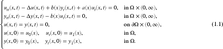
Let be a bounded open domain in with a boundary of class . In Gerbi et al. (2021), the authors have investigated the energy decay of a system of two linear wave equations coupled through velocities described by (see also Alabau-Boussouira et al., 2017 for the case of a nonlinear damping):
where and is a function satisfying
and for a given open subset
Moreover, it is imposed that there exists a non-empty open subset of such that
where is the closure of .
In order to analyze the energy decay properties of system (1.1), the following assumptions have been considered:
The coupling region is contained within the damping region , and satisfies the so-called Geometric Control Condition (GCC), introduced in Bardos et al. (1992) and recalled below in Definition 2.1.
The coupling coefficient is small and positive, satisfying , , where and is a constant depending on the domain and the control region. Additionally, there exists such that almost everywhere in . Moreover, both the coupling region and the damping region satisfy an appropriate geometric condition known as the Piecewise Multipliers Geometric Condition (PMGC), introduced in Liu (1997), applied in Alabau-Boussouira et al. (2017) and recalled below in Definition 2.1.
Under Assumption 1.1, the authors in Gerbi et al. (2021) combined a frequency domain approach with the multiplier technique to establish the exponential decay of the corresponding energy for system (1.1). On the other hand, under Assumption 1.2, the authors in Alabau-Boussouira et al. (2017) employed multiplier techniques to achieve similar exponential stability results.
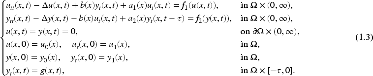
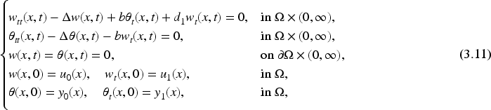
In this work, we aim to extend the results in Alabau-Boussouira et al. (2017), and Gerbi et al. (2021) by considering a more complex setting where the system incorporates a time delay in one equation and nonlinear source terms. Specifically, we investigate the following coupled wave system:
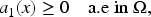
Here, the functions and are given coefficients. The coefficient satisfies the conditions:
and
The initial state belongs to an appropriate function space, which will be specified later. Moreover, and are two nonlinear functions satisfying suitable hypotheses that will be specified in the next sections. Finally, represents the constant time delay.
Unlike previous studies that considered coupled wave systems where both the damping and delay terms appear in the same equation (Akil, Badawi, Wehbe, 2021; Moumni et al., 2024; Oliveira & Oquendo, 2020; Silga et al., 2022), our focus is on the more challenging scenario where the damping and delay are distributed across different equations. This configuration complicates the stability analysis. Indeed, in the classical setting where both mechanisms are in the same equation, the damping can directly counterbalance the delay effects (cf. Nicaise & Pignotti, 2006). In our case, this interaction is not straightforward, leading to additional mathematical challenges. This motivates our investigation into establishing new energy decay results for system (1.3) under appropriate conditions.
Furthermore, we include nonlinear terms in the system, taking into account the presence of source terms. Nonlinear effects are often present in delay differential equations that come from real-life applications. Various works have studied hyperbolic equations with suitable nonlinear source terms. For example, in Ayechi et al. (2025), Chellaoua et al. (2023), Fragnelli and Pignotti (2016), Paolucci and Pignotti (2022), and Pignotti (2024), the authors study the stability of solutions for some abstract wave equations with nonlinear terms satisfying some local Lipschitz continuity assumption. The presence of nonlinear terms makes the models more difficult to deal with and the stability issues require a more sophisticated analysis.
To the best of our knowledge, this is the first work in which the destabilizing effect of a delay feedback present in one equation is compensated by means of a standard frictional damping in the other equation. Moreover, the source terms introduce stability issues too. This combination makes the mathematical analysis more delicate.
Our goal is, then, to explore how the interaction between delay, nonlinearity, damping, and coupling mechanisms influences the stability properties of the system, and to derive sufficient conditions ensuring exponential energy decay.
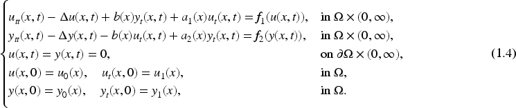
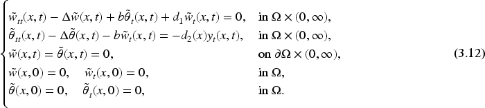
Additionally, we also examine the particular case , which corresponds to a system with indefinite damping:
This system represents a limiting case of our study but is considered separately since we can obtain the result under weaker conditions when . In particular, we establish exponential stability for (1.4) under a suitable assumption on . The study of indefinite damping functions in scalar wave equations has been considered in previous works, such as (Benaddi & Rao, 2000; Freitas & Zuazua, 1996; Haraux, 1989; López-Gómez, 1997; Menz, 2007) but for coupled wave equations has not been done as far as we know.
The Delayed Coupled System
In this section, we analyze the well-posedness and stability of the nonlinear delayed coupled system (1.3). Before presenting our main result of this section, we recall the GCC introduced by Bardos et al. (1992) and the PMGC introduced by Liu (1997).
We say that a subset of satisfies the GCC if there exists a time such that every ray of the geometrical optics starting at any point at enters the region within time .
We say that a subset satisfies the , if there exist subsets with Lipschitz boundaries and points , such that for and contains a neighborhood in of the set , where and is the outward unit normal to .
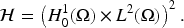
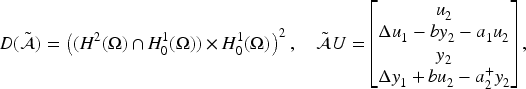
We introduce the energy space
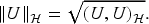
Considering real-valued solutions, is defined as a real Hilbert space equipped with the inner product:
for all and in . The associated norm is given by
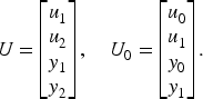
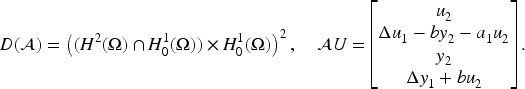
Setting , , , and , we define the state variable
We also introduce
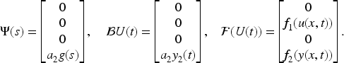
Next, we define the linear operator by
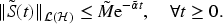
It is well known that the operator is non-negative and generates an exponentially stable contraction semigroup on (see Alabau-Boussouira et al., 2017, Remark 3.3 and Gerbi et al., 2021, Theorem 3.4) under either Assumption 1.1 or Assumption 1.2. More precisely, there exist constants and such that
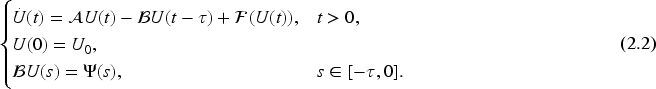
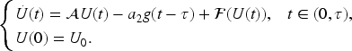
Thus, the delayed coupled system (1.3) can be rewritten in the following abstract form:
In order to study well-posedness and the exponential stability of system (2.2), we make the following assumptions on and :
are continuous functions such that
;
For all there exists a constant such that, for all satisfying and , one has
for ; and as
There exist two strictly increasing continuous functions such that
for all and .
Furthermore, thanks to Hypothesis 2.1, we have that and for any there exists a constant such that
whenever and . In particular,
Let us define
for .
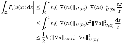
Under Hypothesis 2.1, we derive the following estimates for the nonlinear terms and .
Assume Hypothesis 2.1 holds. Then, for all and , we have
We begin by establishing the local existence and uniqueness of solutions, as stated in the following lemma.
Let us consider the system (2.2) with initial data and Then, there exists a unique continuous local solution defined on a time interval , for some .
Note that for Then, for we have and we can rewrite the abstract system (2.2) as an non-delayed problem:
Then, we can apply the classical theory of nonlinear semigroups (Pazy, 2012) obtaining the existence of a unique solution on a set , with .
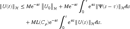
Observe that, for solution to (2.2), the following Duhamel formula holds:
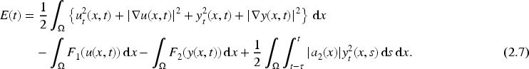
In the spirit of Paolucci and Pignotti (2022), in order to have the existence and uniqueness of a global solution of the system (2.2), we introduce the following energy functional associated to system (1.3):
Let be a mild solution of (1.3) and define its energy by
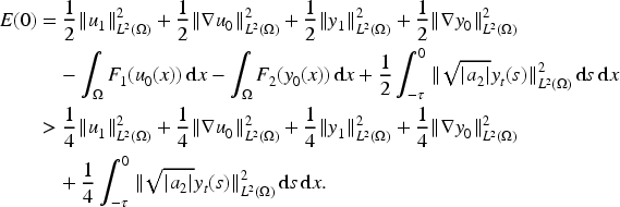
We can deduce a first estimate for small enough initial data.
Assume Hypothesis 2.1. Let be a non-trivial solution of (2.2) defined on an interval for some If and , then .
From Lemma 2.1, we can infer that
and
As a consequence,
Therefore, since is a non-zero solution, we have proven that .
We can also obtain the following preliminary estimate.
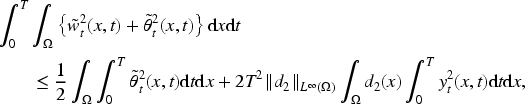
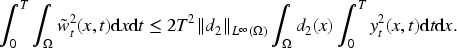
Let be a solution to (1.3) defined on an interval for some If , for any , then
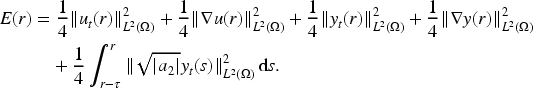
for any , where
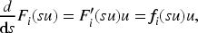
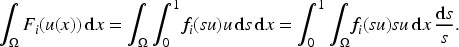
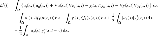
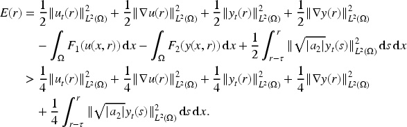
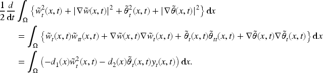
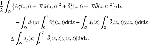
Differentiating formally with respect to , we obtain
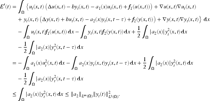
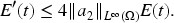
By using the equations satisfied by and in (1.3) and Green formula, we get
Next, we can give the following estimate from below for sufficiently small initial data.
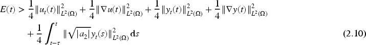
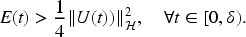
Assume Hypothesis 2.1. Let be a non-trivial solution of (2.2) defined on an interval , and fix a time . Then, if , and for , with defined as in (2.9), then
for all . In particular,
We argue by contradiction. Let us denote
We suppose by contradiction that . Then, by continuity, we have
Then, we can see that
Using the fact that for are increasing functions and Proposition 2.1, we get
and
Hence using the definition of the energy and (2.5), we conclude that
This contradicts the maximality of . Hence, and this concludes the proof of the lemma.
Next, we establish an exponential decay result for the abstract model (2.2) under an appropriate assumption on the function . Let us consider the following hypothesis
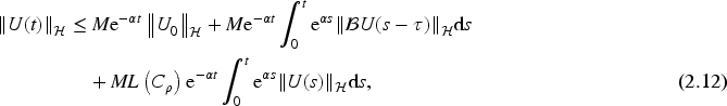
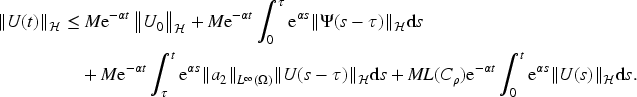
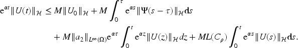
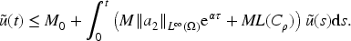
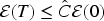
Assume that either Assumption 1.1 or Assumption 1.2 holds, together with Hypotheses 2.1 and 2.2. Let a solution of the system (2.2) satisfying for all with such that . Then, the following exponential decay estimate holds
As before, using Assumption 2.2, we obtain (2.11).
We are now ready to prove the global existence and uniqueness for solutions of system (1.3).
Assume that either Assumption 1.1 or Assumption 1.2 holds, together with Hypotheses 2.1 and 2.2. We consider the initial data and such that
with sufficiently small constant. Then, the problem (2.2) has a unique global solution exponentially decaying according to (2.11).
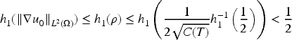
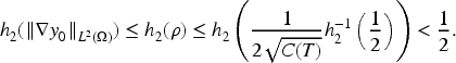
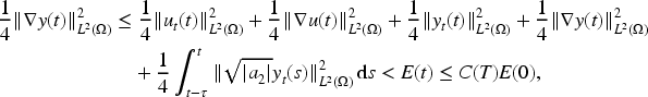
Let us fix a time such that
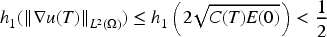
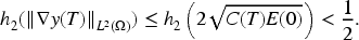
Moreover let be such that
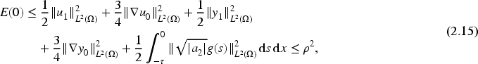
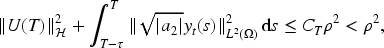
We consider initial data such that
We observe that this is equivalent to
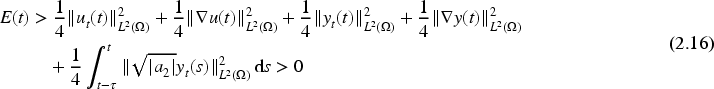
Now, by Lemma 2.2 we know that there exists a local solution of (1.3) on a time interval . Without loss of generality, we can assume (eventually, we can take a larger ). From our assumption on the initial data, on the monotonicity of for and the fact that , we have
and
Hence, by Lemma 2.3, . Moreover, from (2.5), we obtain
which gives us
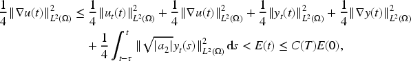
for . Hence, we can apply Lemma 2.4 to obtain
for all ; in particular for all . Thus, applying Proposition 2.1 and the fact that we have
As a consequence, from (2.16) and (2.17), we obtain
and
for all . Then, we can extend the solution in and on the whole interval . In particular, for , we get
We proceed by applying a similar argument as before on the interval , thereby extending the solution to . By iterating this process inductively, we construct a unique global solution to (2.2). Moreover, at each step, the exponential decay estimate (2.11) is preserved, ensuring that the global solution satisfies this decay property.
The Coupled System in the Presence of Indefinite Damping
In this section, we study the problem (1.4). Referring to Section 2, one can reproduce the same procedure in the case when , and deduce that the problem (1.4) is exponentially stable under the following condition on the coefficient :
The main objective of this section is to establish the exponential stability of the problem (1.4) under a weaker condition, namely, by restricting the assumption on the negative part of , that is .
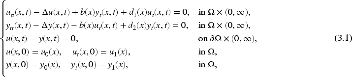
Before addressing problem (1.4), we first need to investigate the exponential stability of the associated coupled wave equation with a definite (i.e., non-negative) damping:
where and are given functions. The coefficient satisfies the conditions
and
While the coefficient satisfies the condition
Next, we define the linear unbounded operator by
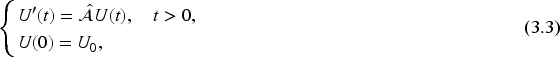
Using this operator, we rewrite the system (3.1) as an abstract Cauchy problem. Indeed, setting , one has that (3.1) can be formulated as
where .
The existence and uniqueness result reads as follows.
For any , there exists a unique solution of system (3.3). Moreover, if , then
We will prove that the operator defined in (3.2) generates a contraction semi-group on the Hilbert space . To this end, we show that the unbounded operator is maximal dissipative on . According to Cazenave and Haraux (1998, Proposition 2.2.6), it is sufficient to prove that is dissipative and that is surjective, where
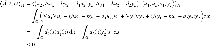
. Let . Then, by integrating by parts and due to the fact that and , we obtain
Therefore the operator is dissipative.
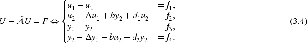
is surjective. Given , we seek such that
We suppose that we have found and with the right regularity. Then, we set
Eliminating and in (3.4), we get the following system
Now, we consider the bilinear form given by
and the linear form given by
In view of Poincaré inequality, is a continuous bilinear form on and is a continuous linear functional on . Moreover, it is easy to check that is also coercive on . Indeed, let
By applying the Lax–Milgram theorem, we deduce that there exists a unique solution of
If , then solves (3.6) in and so (See Allaire, 2009, Chapter 5). Now, take ; then . Thus, we have found , which satisfies (3.4). Consequently is surjective. Conclusively, the Lumer–Phillips Theorem implies the operator generates a strongly continuous semigroup of contraction in . Consequently, the well-posedness result follows from the Hille-Yosida theorem (see Barbu, 1998, Theorem 4.5.1 or Coron, 2007, Theorem A.11).
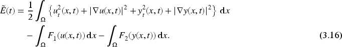
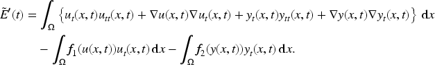
Now, we study the exponential stability of system (3.1). To this aim we first define its corresponding energy by
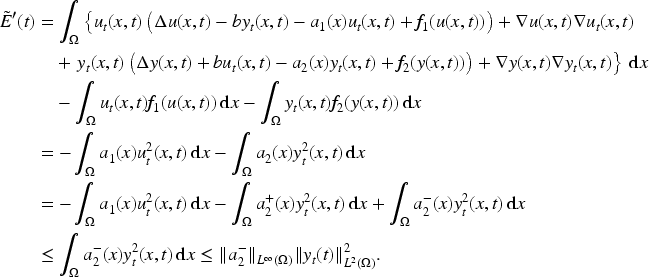
Direct computations allow to show that the energy exhibits a decay with respect to time. More precisely, we have the following result. The energy associated to the solution of system (3.1) satisfies
Consequently, the energy is nonincreasing.
We can prove the following exponential stability result for the problem (3.1).
Assume that either Assumption 1.1 or Assumption 1.2 holds. There exist two positive constants such that
Thus, as a direct consequence of Haraux (1989, Proposition 2), it follows that under either Assumption 1.1 or Assumption 1.2, the exponential stability property given by (2.1) implies the existence of a constant time such that, for every , the following holds:
This easily implies the stability estimate (3.10), since our system (3.1) is invariant by translation and the energy is decreasing.
Returning to the problem (1.4), and using the same notations as those introduced in Section 2, we define the linear operator by
where denotes the positive part of the function , defined by
By applying Theorem 3.2 with and , we deduce that the operator is non-negative and generates a contraction semigroup on , which is exponentially stable under either Assumption 1.1 or Assumption 1.2. More precisely, there exist constants and such that
Consequently, the coupled system (1.4) can be reformulated as the following abstract Cauchy problem:
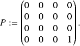
where is the linear projection operator defined by
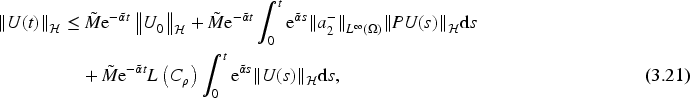
Observe that, if , then the following Duhamel formula holds:
Using Cazenave and Haraux (1998, Proposition 4.3.3), we can establishing the local existence and uniqueness of solutions, as stated in the following lemma.
Let . Then, the system (3.14) has a unique continuous local solution defined on a time interval .
Let us introduce the following energy functional associated to system (3.14):
Let be a mild solution of (1.4). Let us define its energy by
By arguing as in the proof of Lemma 2.3, we can establish the following result concerning the indefinite damping case.
Assume that Hypothesis 2.1 holds. Let be a non-trivial solution of the problem (3.14), defined on the interval If the initial data satisfy
then the initial energy is strictly positive, that is, .
Using Proposition 3.1 and adapting the arguments used in the proof of Lemma 2.4, we obtain the following result concerning the lower bound of the energy in the presence of indefinite damping.
Assume that Hypothesis 2.1 holds. Let be a non-trivial solution of problem (3.14), defined on the interval and fix a time .
Suppose the initial data satisfy the following conditions:
Then, the energy satisfies the following strict lower bound for all :
In particular, one has:
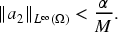
Next, we establish an exponential decay result for the abstract system (3.14) under a weaker condition on the damping coefficient . More precisely, we impose a smallness assumption only on the negative part of . To this end, we introduce the following hypothesis:
The function satisfies
Under this assumption, we prove that the solution to (3.14) decays exponentially in time. This is stated precisely in the following theorem.
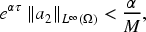
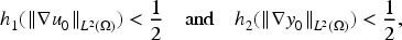
Assume that either Assumption 1.1 or Assumption 1.2 holds, together with Hypotheses 2.1 and 3.1. Let be a solution of the problem (3.14) satisfying the uniform bound
for some constant such that
where is the Lipschitz constant of the nonlinearity as defined in Hypothesis 2.1.
Then, the following exponential decay estimate holds:
As before, using Assumption 3.1, we obtain (3.20).
We are now in a position to establish the global well-posedness and the exponential decay estimates for solutions to (1.4) corresponding to small initial data.
Assume that either Assumption 1.1 or Assumption 1.2 holds, together with Hypotheses 2.1 and 3.1. Let the initial data satisfy
for a sufficiently small constant . Then, the Cauchy problem (3.14) admits a unique global solution which decays exponentially in time according to estimate (3.20).
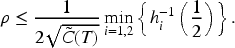
Let us fix , such that
Moreover let be such that
We consider initial data satisfying
By Lemma 3.1, there exists a local solution to (1.4) on some interval , with . Without loss of generality, we may assume .
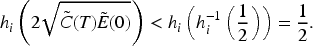
Using the monotonicity of and the fact that , we obtain
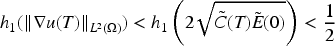
Therefore, by Lemma 3.2, we have . Moreover, from estimate (2.5), it follows that
This implies, for ,
Hence, applying Lemma 3.3, we obtain the energy lower bound
From Proposition 3.1 and the fact that , we deduce
Thus, we can iterate the argument on successive intervals , , and so on. By induction, we construct a unique global solution to (3.14). Furthermore, at each step, the exponential decay estimate (3.20) is preserved, ensuring that the global solution satisfies this decay property.
Footnotes
Acknowledgments
This work was started when AM was visiting the University of L’Aquila. AM thanks the MAECI (Ministry of Foreign Affairs and International Cooperation, Italy) for funding that greatly facilitated scientific collaborations between Moulay Ismail University of Meknes (Morocco) and University of L’Aquila (Italy).
ORCID iDs
Alhabib Moumni
Cristina Pignotti
Jawad Salhi
Funding
The authors disclosed receipt of the following financial support for the research, authorship, and/or publication of this article: CP is a member of Gruppo Nazionale per l’Analisi Matematica, la Probabilità e le loro Applicazioni (GNAMPA) of the Istituto Nazionale di Alta Matematica (INdAM). She is partially supported by PRIN 2022 (2022238YY5) Optimal control problems: analysis, approximation and applications, PRIN-PNRR 2022 (P20225SP98) Some mathematical approaches to climate change and its impacts, and by INdAM GNAMPA Project Optimal Control and Machine Learning (CUP E5324001950001).
Declaration of Conflicting Interests
The authors declared no potential conflicts of interest with respect to the research, authorship, and/or publication of this article.
References
1.
AdimyM.CrausteF. (2003). Global stability of a partial differential equation with distributed delay due to cellular replication. Nonlinear Analysis: Theory, Methods & Applications, 54, 1469–1491. 10.1016/S0362-546X(03)00197-4
2.
AkilM.BadawiH.NicaiseS.WehbeA. (2021). Stability results of coupled wave models with locally memory in a past history framework via nonsmooth coefficients on the interface. Mathematical Methods in the Applied Sciences, 44, 6950–6981. 10.1002/mma.7235
3.
AkilM.BadawiH.WehbeA. (2021). Stability results of a singular local interaction elastic/viscoelastic coupled wave equations with time delay. Communications on Pure and Applied Analysis, 20, 2991–3028. 10.3934/cpaa.2021092
4.
Alabau-BoussouiraF. (2002). Indirect boundary stabilization of weakly coupled hyperbolic systems. SIAM Journal on Control and Optimization, 41, 511–541. 10.1137/S0363012901385368
5.
Alabau-BoussouiraF. (2003). A two level energy method for indirect boundary observability and controllability of weakly coupled hyperbolic systems. SIAM Journal on Control and Optimization, 42, 871–906. 10.1137/S0363012902402608
6.
Alabau-BoussouiraF. (2013). A hierarchic multi-level energy method for the control of bidiagonal and mixed -coupled cascade systems of PDEs by a reduced number of controls. Advances in Differential Equations, 18, 1005–1072. 10.57262/ade/1378327378
7.
Alabau-BoussouiraF.CannarsaP.SforzaD. (2008). Decay estimates for second order evolution equations with memory. Journal of Functional Analysis, 254, 1342–1372. 10.1016/j.jfa.2007.09.012
8.
Alabau-BoussouiraF.LéautaudM. (2013). Indirect controllability of locally coupled wave-type systems and applications. Journal de Mathematiques Pures et Appliquees, 99, 544–576. 10.1016/j.matpur.2012.09.012
9.
Alabau-BoussouiraF.WangZ.YuL. (2017). A one-step optimal energy decay formula for indirectly nonlinearly damped hyperbolic systems coupled by velocities. ESAIM: Control, Optimisation and Calculus of Variations (ESAIM: COCV), 23, 721–749. 10.1051/cocv/2016011
10.
AllaireG. (2009). Analyse numérique et optimisation. Éditions de l’École Polytechnique.
11.
AmmariK.ChentoufB.SmaouiN. (2022). Well-posedness and stability of a nonlinear time-delayed dispersive equation via the fixed point technique: A case study of no interior damping. Mathematical Methods in the Applied Sciences, 45, 4555–4566. 10.1002/mma.8052
12.
AmmariK.NicaiseS.PignottiC. (2010). Feedback boundary stabilization of wave equations with interior delay. Systems & Control Letters, 59, 623–628. 10.1016/j.sysconle.2010.07.007
13.
AvdoninS.RiveroA. C.de TeresaL. (2013). Exact boundary controllability of coupled hyperbolic equations. International Journal of Applied Mathematics and Computer Science, 23, 701–710. 10.2478/amcs-2013-0052
14.
AyechiR.KhenissiM.LaurentC. (2025). Indirect stabilization of semilinear coupled wave system. Mathematical Control and Related Fields (MCRF), 15, 493–514. 10.3934/mcrf.2024021
15.
BarbuV. (1998). Partial differential equations and boundary value problems. Kluwer Academic Publishers.
16.
BardosC.LebeauG.RauchJ. (1992). Sharp sufficient conditions for the observation, control and stabilization of waves from the boundary. SIAM Journal on Control and Optimization, 30, 1024–1065. 10.1137/0330055
17.
BenaddiA.RaoB. (2000). Energy decay rate of wave equations with indefinite damping. Journal of Differential Equations, 161, 337–357. 10.1006/jdeq.2000.3714
18.
BennourA.Ammar KhodjaF.TeniouD. (2017). Exact and approximate controllability of coupled one-dimensional hyperbolic equations. Evolution Equations and Control Theory, 6, 487–516. 10.3934/eect.2017025
19.
BerrimiS.MessaoudiS. A. (2006). Existence and decay of solutions of a viscoelastic equation with a nonlinear source. Nonlinear Analysis: Theory, Methods & Applications, 64, 2314–2331. 10.1016/j.na.2005.08.015
20.
CazenaveT.HarauxA. (1998). An introduction to semilinear evolution equations. Oxford University Press.
21.
ChellaouaH.BoukhatemY.FengB. (2023). Well-posedness and stability for an abstract evolution equation with history memory and time delay in hilbert space. Advances in Differential Equations, 28, 953–980. 10.57262/ade028-1112-953
22.
ContinelliE.PignottiC. (2025). Energy decay for semilinear evolution equations with memory and time-dependent time delay feedback. Advances in Differential Equations, 30, 601–634. 10.57262/ade030-0910-601
23.
CoronJ.-M. (2007). Control and nonlinearity. American Mathematical Society.
24.
DatkoR. (1991). Two questions concerning the boundary control of certain elastic systems. Journal of Differential Equations, 92, 27–44. 10.1016/0022-0396(91)90062-E
25.
FragnelliF.PignottiC. (2016). Stability of solutions to nonlinear wave equations with switching time delay. Dynamics of Partial Differential Equations, 13, 31–51. 10.4310/DPDE.2016.v13.n1.a2
26.
FreitasP.ZuazuaE. (1996). Stability results for the wave equation with indefinite damping. Journal of Differential Equations, 132, 338–352. 10.1006/jdeq.1996.0183
27.
GerbiS.KassemC.MortadaA.WehbeA. (2021). Exact controllability and stabilization of locally coupled wave equations: Theoretical results. Zeitschrift für Analysis und ihre Anwendungen, 40, 67–96. 10.4171/zaa/1673
28.
HarauxA. (1989). Une remarque sur la stabilisation de certains systemes du deuxieme ordre en temps. Portugaliae Mathematica, 46, 245–258. https://eudml.org/doc/115668
LiuK. (1997). Locally distributed control and damping for conservative systems. SIAM Journal on Control and Optimization, 35, 1574–1590. 10.1137/S0363012995284928
31.
LiuZ.RaoB. (2009). A spectral approach to the indirect boundary control of a system of weakly coupled wave equations. Discrete & Continuous Dynamical Systems, 23, 399–414. 10.3934/dcds.2009.23.399
32.
López-GómezJ. (1997). On the linear damped wave equation. Journal of Differential Equations, 134, 26–45. 10.1006/jdeq.1996.3209
33.
LuoJ. R.XiaoT. J. (2023). Optimal decay rates for semi-linear non-autonomous evolution equations with vanishing damping. Nonlinear Analysis: Theory, Methods & Applications, 230. Paper No. 113247. 10.1016/j.na.2023.113247
34.
MenzG. (2007). Exponential stability of wave equations with potential and indefinite damping. Journal of Differential Equations, 242, 171–191. 10.1016/j.jde.2007.04.002
35.
MokhtariY.Ammar KhodjaF. (2022). Boundary controllability of two coupled wave equations with space-time first-order coupling in 1-D. Journal of Evolution Equations, 22. Paper No. 31. 10.1007/s00028-022-00790-x
36.
MoumniA.MehdaouiM.SalhiJ.TiliouaM. (2024). Theoretical and numerical indirect stabilization of coupled wave equations with a single time-delayed damping. arXiv:2410.09995.
37.
NicaiseS.PignottiC. (2006). Stability and instability results of the wave equation with a delay term in the boundary or internal feedbacks. SIAM Journal on Control and Optimization, 45, 1561–1585. 10.1137/060648891
38.
OliveiraR. L.OquendoH. P. (2020). Stability and instability results for coupled waves with delay term. Journal of Mathematical Physics, 61, 071505. 10.1063/1.5144987
39.
PaolucciA.PignottiC. (2022). Well-posedness and stability for semilinear wave-type equations with time delay. Discrete & Continuous Dynamical Systems-Series S, 15, 1561–1571. 10.3934/dcdss.2022049
40.
PazyA. (2012). Semigroups of linear operators and applications to partial differential equations. Springer.
41.
PignottiC. (2012). A note on stabilization of locally damped wave equations with time delay. Systems & Control Letters, 61, 92–97. 10.1016/j.sysconle.2011.09.016
42.
PignottiC. (2024). Exponential decay estimates for semilinear wave-type equations with time-dependent time delay. arXiv:2303.14208.
43.
RebiaiS. E.Sidi AliF. Z. (2014). Exponential stability of compactly coupled wave equations with delay terms in the boundary feedbacks. In System Modeling and Optimization: 26th IFIP TC 7 Conference, CSMO 2013, Klagenfurt, Austria, September 9–13, 2013, Revised Selected Papers (pp. 278–284). Springer.
44.
SilgaR.KyelemB. A.BayiliG. (2022). Indirect boundary stabilization with distributed delay of coupled multi-dimensional wave equations. Annals of the University of Craiova-Mathematics and Computer Science Series, 49, 15–34. 10.52846/ami.v49i1.1430
45.
WehbeA.YoussefW. (2011). Indirect locally internal observability and controllability of weakly coupled wave equations. Difference Equations and Applications, 3, 449–462.
46.
XuG. Q.YungS. P.LiL. K. (2006). Stabilization of wave systems with input delay in the boundary control. ESAIM: Control, Optimisation and Calculus of Variations, 12, 770–785. 10.1051/cocv:2006021
47.
XuG. Q.ZhangL. (2020). Uniform stabilization of 1-D coupled wave equations with anti-dampings and joint delayed control. SIAM Journal on Control and Optimization, 58, 3161–3184. 10.1137/19M1289145
48.
ZuazuaE. (1990). Exponential decay for the semilinear wave equation with locally distributed damping. Communications in Partial Differential Equations, 15, 205–235. 10.1080/03605309908820684