
Abstract
We consider a behavioral model of voting in multi-candidate elections under plurality rule. In the case of a positive impression of the campaign leader, voters increase their propensity to vote for that candidate, while in the case of a negative impression voters decrease their propensity. The formation of positive or negative impressions depends on an endogenous aspiration level. We show that in multi-candidate elections, in any stationary distribution, the winner receives a share of 50% of votes. Our results suggest that achieving coordination is ‘path-dependent’: whether voters manage to coordinate on the majority-preferred candidate critically depends on the initial state. We then identify conditions that make the election of the majority-preferred candidate more likely. However, even if the majority candidate is elected for sure, voting behavior is only partially coordinated.
1. Introduction
Game-theoretic models of voting have demonstrated the strategic complexity of multi-candidate elections (e.g., Cox, 1994, 1997; Fey, 1997; Myatt, 2007; Myatt and Fisher, 2002a,b; Myerson and Weber, 1993; Palfrey, 1989). In the canonical model, candidates have fixed policy positions, while voters are assumed to maximize their expected policy payoff based on the election outcome. Despite its apparent simplicity, the model is difficult to analyze. This is because voters who prefer a badly trailing candidate have an incentive to abandon their first choice who is likely to lose, and switch their vote to a more competitive candidate. This ‘no-wasted-votes’ argument requires that voters form expectations about the likelihood that a candidate will win and then vote for the candidate who maximizes their expected utility. However, these expectations themselves depend on the expected vote choices of the entire electorate, which depend on the electorate’s expectations about who is leading, and so forth. In equilibrium, voters are assumed to calculate the probability of being pivotal among low-probability events and to base their decisions on relative pivot probability ratios.
A long tradition in political science has questioned the empirical validity of such models of strategic voting. 1 According to this literature, not only do voters lack basic information or coherent policy positions, their reasoning processes are heavily biased and bear no resemblance to the rational cognitive processes presumed by game-theoretic models (e.g., Achen and Bartels, 2002, 2016; Berelson et al., 1954; Campbell et al., 1960; Cole et al., 2012; Healy and Lenz, 2014; Healy et al., 2010; Stimson, 2004; Wolfers, 2002). Following these findings, some scholars have suggested that voters essentially vote how they ‘feel’ and that this lack of sophistication can have dire consequences for democratic governance, as elections amount to little else than random selection devices driven by biases and politically irrelevant factors (e.g., Achen and Bartels, 2004, 2016). Such sweeping normative conclusions, in turn, have led to rebuttals from rational choice theorists. Counter-arguments have questioned the empirical validity of behavioral criticisms of rational choice models or defended the explanatory power of existing rational choice models. (e.g., Ashworth, 2012; Ashworth and de Mesquita, 2014).
In this paper, we take a different approach. We set aside the empirical debate on the extent of voter rationality, information, or competence. Instead, we will formally explore the performance of electoral institutions if voters indeed act as described by, e.g., Achen and Bartels (2016) and vote ‘as they feel.’ Specifically, we assume that voting behavior is consistent with one of the fundamental principles of learning theory, the law of effect (Hilgard and Bower, 1966; Thorndike, 1898): actions that are associated with favorable impressions are more likely to occur; those that are associated with negative impressions are less likely to occur. According to this view, rather than using best-response strategies based on rationally formed beliefs, voters adapt their voting propensities in response to positive and negative impressions, which are compared with an aspiration level based on past impressions (Bendor et al., 2003, 2011; Karandikar et al., 1998). In the case of a positive impression of a candidate, i.e., an impression above their aspiration level, voters increase their propensity to vote for the candidate; while in case of negative impression of a candidate, i.e., an impression below their aspiration, voters decrease their propensity for the candidate and shift their voting propensity to the other candidates. Aspiration levels are not fixed but incorporate past impressions. This behavioral rule requires far less cognitive effort, attention, and ability than the classical game-theoretic approach, in which voters make decisions based on complex pivot events that occur with very small probabilities. Moreover, voters are not assumed to know the details of their environment, such as the action sets of other voters, the details of opinion polls, or even the fact that voters adjust their propensities based on impressions, and so forth.
We then apply this model to the problem of candidate selection in multi-candidate elections. That is, voters elect a public representative from a finite list of candidates with fixed policy positions under plurality rule. In contrast to the negative assessment of Achen and Bartels (2004), we find that, even if voters vote ‘as they feel,’ elections perform quite well. In a two-candidate case, the majority-preferred candidate always wins. We then consider the case of multiple candidates. We first show that the voting process is, in general, path-dependent: whether voters are able to coordinate on a majority-preferred candidate (and on which of the candidates) depends on the initial state. 2 We then show that a majority-preferred candidate wins under a broad set of circumstances even if voters simply rely on fleeting impressions of candidates.
While the main focus of the paper is on analyzing the normative properties of elections with behavioral voters, our paper also makes a methodological contribution. Aspiration-based behavioral models are often difficult to solve analytically. In their analysis of the prisoners’ dilemma, Karandikar et al. (1998), for example, are only able to analyze
2. The model
There are n candidates with fixed policy positions. Elections are conducted by plurality rule. The set of all candidates will be denoted by
The second factor,
The intended domain of our model is an electoral campaign. In each period t (
In each period t, the voting propensities of the electorate determine who is the leading candidate, the ‘campaign leader,’ and who are the ‘campaign laggards.’ This can be done through a poll or media reports. Voters base their propensities solely on who is the campaign leader. They do not pay any attention to other features of the race, such as expected vote shares in an election poll and do not use Bayes’ rule to form beliefs about the likely outcome of the race, in contrast with the approaches proposed in Diermeier and Van Mieghem (2008) and Fey (1997). This formally captures the notion of inattentive, uninformed, and uninterested voters, a feature often pointed out by the behaviorally oriented political science literature on electoral campaigns (e.g., Stimson, 2004). The details of the adjustment process are presented in the next subsection.
2.1. The behavioral adjustment process
The adjustment process is a generalization of the model proposed in Bendor et al. (2003) and Karandikar et al. (1998). As a convention, we will use superscripts to denote time and subscripts to denote voters and voter types. In addition, we use brackets to refer to candidates. As an example,
In each period t, each voter forms an impression about the campaign leader given by
As in Bendor et al. (2003) and Karandikar et al. (1998), the aspiration level
The specific rules used to adjust voting probabilities and aspirations are as follows.
2.1.1. Voting probabilities adjustment
Voting probabilities evolve according to the Bush–Mosteller rule (Bendor et al., 2003, 2011; Bush and Mosteller, 1955; Karandikar et al., 1998). Specifically:
Suppose candidate i, with

Suppose candidate i, with

Under the Bush–Mosteller rule, the new propensity
2.1.2. Aspiration adjustment
Aspirations evolve according to the Cyert–March rule (Bendor et al., 2003, 2011; Cyert and March, 1963; Karandikar et al., 1998), defined as

where
Under the Cyert–March rule, the aspiration,
3. Stationary distributions and normative implications
The basic model and the behavioral process described in Section 2.1 jointly define a dynamic process. Our goal is to characterize the stationary distributions of that adjustment process and its properties. Specifically, we focus on a two-candidate election, and a well-studied three-candidate election, called ‘beat the incumbent’ (e.g., Fey (1997); Myatt (2007); Myatt and Fisher (2002b); Myerson and Weber (1993).
3.1. Two-candidate elections
We first consider the case of n=2 candidates. In rational choice models of voting, this is a trivial case as voters simply vote for their preferred candidate. In a behavioral model where voters are inattentive and vote based on their impressions, this may not be the case. Specifically, we wish to explore the claim of Achen and Bartels (2004) that if voters vote ‘how they feel,’ elections amount to little less than a ‘random oligarchy.’ The case of n=2 will also illustrate the logic of impression-based voting in general. Later, we will extend this analysis to multi-candidate elections.
Suppose there are two candidates, candidate A and candidate B, and two types of voter:
The analysis proceeds as follows. Consider a stationary distribution in which, say, candidate A is the campaign leader. In this case, the voter’s impression
A similar argument applies at the other stationary distribution, in which candidate B is the expected winner. The predicted shares of the two candidates will be 50% each. But, whenever A is expected to win, given the larger share of AB voters, the share of votes that A receives will shoot above 50%, again with the increase being dependent on the share of AB voters. It therefore follows that since AB voters are more numerous than BA voters, the share of votes that candidate A is expected to receive can never go below 50%, and, on average, will exceed 50%, with its level being dependent on the size of its supporters in the electorate.
We summarize this result in the following proposition. The proof is straightforward and thus omitted.
Note that the vote share received by A is proportional, but in general not equal, to the size of the AB faction. More specifically, the voting behavior is such that a majority of AB voters will vote for A, and similarly, a majority of BA voters will vote for B; while, on aggregate, A will be the expected winner of the election as desired by a majority. Thus, voters typically do not ‘vote sincerely’ or ‘expressively’ (Schuessler, 2000), but the dynamics of the adjustment process ensure that the majority-preferred candidate wins.
3.2. The ‘beat the incumbent’ election
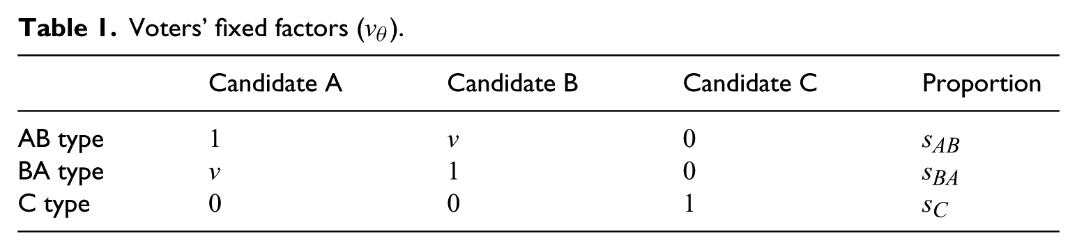
The ‘beat the incumbent’ model (e.g., Fey, 1997; Myatt, 2007; Myatt and Fisher, 2002b; Myerson and Weber, 1993) consists of three candidates A, B, and C, and three types of voter: AB, BA, and C. The labels indicate the top preferences of each type, for example an AB type prefers A over B, and B over C. AB and BA voters both rank candidate C third and thus have a common interest in making sure that C does not get elected, though their preferences diverge on who they rank first. The fixed factors v of each type are described in Table 1. v is a parameter with
Voters’ fixed factors (
In the ‘beat the incumbent’ election, with three candidates, the process allows for multiple stationary distributions. Yet, all attainable stationary distributions can be characterized in the following proposition. 6
Proof. In the appendix. □
The intuition for the result is as follows. Consider a stationary distribution and suppose that candidate A is the sole winner. In this case, the distribution of impressions is
To see why the winner must receive a share of 50%, suppose, by way of contradiction, that his share is below 50%. First we note that, since the population is continuous, the winner’s share (in this case candidate A) is exactly the aggregate probability of voting for candidate A across the entire electorate. Thus, a share of less than 50% for candidate A is equivalent to an aggregate chance of voting for candidate A below 0.5. Second, since the (aggregate) likelihood of voting for candidate A is less than 0.5, the Bush–Mosteller rule implies that, on average, the probability increase of voters with a positive impression of candidate A will be larger than the probability decrease of voters with a negative impression. As voters with positive and negative impressions are split 50%–50%, the probability of voting for candidate A will, on average, increase. Thus, the share of candidate A will increase, which contradicts the stationarity assumption. A similar reasoning shows that if candidate A’s share is above 50% then, on average, the probability of voting for candidate A decreases. Alternatively, the share of candidate A decreases, which, again, is contrary to the stationarity assumption. Therefore, the only candidate for a stationary distribution is a state in which candidate A receives 50% votes. Indeed, at an average voting inclination of 0.5 (which is equivalent to a share of 50% votes for candidate A) the adjustments of voters with positive and negative impressions of candidate A will compensate each other and the distribution will be stationary.
Note that Proposition 2 holds at the aggregate level, i.e., at the level of types, not at the individual voter level. Specifically, voters attach voting probability 0.5 to voting for the winning candidate only on average. In contrast, individual voting propensities will vary across voters, i.e., some voters will be more likely to vote for the winning candidate, others less likely.
Note also that the prediction of a 50% vote share should not be interpreted too literally. It is a consequence of our mathematical assumption of a continuum of voters. In any finite electorate, we would have a distribution over vote shares centered around 50%. Proposition 2 is thus consistent with the electoral data from the 1987–1997 parliamentary elections in England analyzed by Myatt and Fisher (2002a,b): the distribution of vote shares of the winning candidates is single-peaked and centered around 50%. 7
The model allows for multiple stationary distributions, one for each candidate. All stationary distributions allocate a vote share of 50% to the winning candidate and the adjustment process uniquely selects one of the stationary distributions, but which one depends on the process’ starting state. That is, the result is properly viewed as a form of ‘path-dependence.’ 8 This naturally raises the question under what circumstances the plurality-preferred candidate will be elected. We will discuss this question in Section 3.2.1.
3.2.1. Path-dependency and coordination success
Proposition 2 implies that the adaptive process is path-dependent. That is, it is possible for each candidate to be the election winner, including the Condorcet loser. Proposition 2, however, does not tell us how likely these outcomes are. Note also that Proposition 2 does not impose any restrictions on how the voting weights are adjusted for the campaign laggards. To study the path-dependence of the process, we need to be more specific and make assumptions on the way voting weights adjust for all candidates and not only for the campaign leader. We will focus on a class of adjustment rules that satisfy a ‘no-leap-frog’ condition. 9
Intuitively, Assumption 1 requires that any redistribution of vote shares must be balanced, i.e., no campaign laggard is arbitrarily favored. To understand the impact of the condition, consider the following example. Suppose that in the current period, A is the campaign leader, i.e., candidate A has the largest share among the three candidates. Further, suppose that after voters adjust their voting weights, A’s share increases in the next period. Then, we require that A continue to lead.
We now investigate the question under which conditions a majority is successful in coordinating, i.e., elect one of the majority-preferred candidates. Here, we focus on the case where
Proof. In the appendix. □
In other words, if voters initially vote for their preferred choice and aspirations are in a medium range around
It is important to understand two factors that matter in Proposition 3. First, a candidate must be the initial campaign leader. In Proposition 3, the plurality-preferred candidate will be the leader because, by assumption, all voters initially choose their most preferred candidate. Second, that initial success must be amplified. Various factors play a role here. One of them is the fact that initial aspirations are sufficiently low; another that the systematic support in the voting population must be sufficiently high.
We can further investigate these factors by considering alternative initial conditions. For example, consider the case where there is no initial propensity for the preferred candidate. That is, suppose initial voting probabilities are all equal, i.e.,
Proof. In the appendix. □
Under these assumptions, a candidate with minority support can win the election, provided he is the initial campaign leader and his support is not too small. Intuitively, the condition ‘
We can make this threshold value precise. Specifically, for candidate A’s support to be sufficiently large,
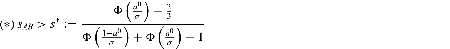
Observe that if
In the next proposition, we state conditions that ensure the success of a majority-preferred candidate, i.e., A or B.
11
This will depend on the benefit of coordinating v. That is,
This result indicates that coordination among AB and BA types is more likely if the benefit of coordinating, i.e., parameter v, is large. The intuitive reason is that if v is large, AB voters (or BA) will have a positive impression of B (or A) with a higher probability, because the impression
3.2.2. Duvergerian equilibria and Duverger’s law
We will now compare our analysis of the ‘beat the incumbent’ game with its rational voter analog. Various papers (see, e.g., Fey, 1997; Myerson and Weber, 1993; Palfrey, 1989) show that with rational voters there are three equilibria that fit into two categories. The first category, referred to as ‘Duvergerian,’ in reference to Duverger’s law (Duverger, 1954), includes two equilibria in which the groups of AB and BA voters fully coordinate their votes on either A or B, while the C voters cast their support for C. In this case, only two candidates get votes and A or B wins the election. The second category, referred to as ‘non-Duvergerian,’ includes an equilibrium, in which each group of voters cast their support for their top choice, i.e., AB voters vote for A, BA voters vote for B, and C voters vote for C. In this case, the groups of AB and BA do not coordinate and all three candidates get votes.
From a normative point of view, Duvergerian equilibria are desirable, since the majority faction successfully coordinates on A or B. However, a unique selection of Duvergerian equilibria (and hence a strict derivation of Duverger’s law from a game-theoretic model) has proven to be difficult, since both type of equilibria (Duvergerian or non-Duvergerian) are consistent with the game’s incentives, without any prediction about their relative frequency. Myerson and Weber (1993, p.106) state this as: ‘Duverger’s law cannot be derived exclusively from analysis of voting equilibria. [
To resolve these difficulties, Fey (1997) proposed a model of myopic best-responses dynamic where voters use Bayes’ rule to infer each candidate’s chances of winning based on current opinion polls. Fey’s adjustment model generically converges on a Duvergerian equilibrium for any initial state of the process. Fey thus concludes that the non-Duvergerian equilibrium is ‘unstable.’
In contrast, our model is based on very different behavioral assumptions. In our model, voters do not use best-response strategies; rather they use an adjustment process based on whether their impression of a candidate was positive given their aspiration level. Voters also do not need to know the details of polls or be able to calculate a candidate’s chances of winning using Bayes’ rule. All they need to know is who the leading candidate is. They also do not need to know the details of their environment, such as the presence or action sets of other voters, or the process of impression formation and voting.
Proposition 2 implies that the behavioral adjustment process has three stationary distributions: in two of them, one of the majority candidates (A or B) wins with a share of 50%, while in the third stationary distribution the minority candidate (candidate C) wins, again, with a share of 50%. These predictions may seem similar to those of the game-theoretic model previously discussed; however, there are major differences between the two models, in regard to both the dynamics of the adjustment process and the voting behavior associated with these outcomes. Importantly, there are no ‘unstable’ states in our approach. In particular, as we have seen, the distribution in which the minority candidate C wins can be reached from a large range of starting states. Thus, in our model, the case in which C wins does not constitute an ‘exceptional’ case (as suggested by Palfrey (1989)).
More generally, our model is incompatible with equilibrium behavior in a game-theoretic model.
Conversely, the non-Duvergerian type equilibrium, in which all three candidates receive positive shares of votes, is not stationary either.
These results follow directly from Proposition 2. Proposition 2 states that in any stationary distribution the winner receives a share of 50% of total votes, and, moreover, as shown in the proof, each group of voters will vote for the winning candidate with probability 0.5. But this immediately rules out the two types of equilibria as potential candidates for a stationary distribution. For example, in the Duvergerian equilibrium in which either A or B wins, all C types attach weight zero to voting for A or B, contradicting the voting behavior implied by Proposition 2. Similarly, in the non-Duvergerian equilibrium in which C wins, all AB types put zero mass probability on voting for C. This is inconsistent with Proposition 2.
More generally, no outcome in which one of the candidates receives (exactly)
Whether these differences from the game-theoretic models constitute a vice or a virtue depends on the empirical adequacy of the model. Most theoretical research has identified Duverger’s law with the selection of Duvergerian equilibria. The focus on selecting Duvergerian equilibria, however, has been questioned in recent empirical and theoretical analyses. Cox (1997) and especially Myatt and Fisher (2002a,b) have argued that third-party candidates receive consistently more votes than predicted by Duvergerian equilibria. According to these findings, coordination under plurality rule is partial, as in our model, but in contrast with the properties of Duvergerian equilibria. 14 More empirical research is needed to investigate these issues in detail.
4. Conclusions
A long tradition of voting behavior in political science has suggested that voters are heavily influenced by how they currently ‘feel’ about a candidate and do not engage in rational belief formation or decision-making. We formally capture this view with a model of voting where actions are based on the comparison between voters’ current impression of a candidate and an aspiration level leading to reinforcement-based behavior that has been widely supported by psychological research.
The model defines a dynamic process, and we solve for the stationary distributions of the process. All stationary distributions are of the same form, with one of the candidates winning a majority of votes. In a two-candidate competition, the majority-preferred candidate always wins. In the case of a multiple candidate, the process exhibits path-dependence as, under certain conditions, the initial campaign leader may become the eventual winner.
The dynamics of our model are fundamentally different from the equilibria identified by game-theoretic models or best-response-based adjustment models, as in Fey (1997). Winning an election depends on initial success plus amplification of support, which depends on the attitudes of the electorate. It is possible for a minority-preferred candidate to be elected, provided he leads in the first round and has sufficient support in the electorate. But the likelihood that a majority candidate will be elected will increase if the candidate commands a larger support in the electorate and the benefits of coordination among the majority factions are large. Moreover, low initial aspirations make it easier for a majority candidate to win, provided he has significant initial support.
In our model, a substantial segment of the voting population do not vote according to their preferences. That is, they do not vote ‘sincerely.’ This concentration of support, however, is not due to ‘strategic voting,’ if by that term we mean a conscious calculation based on relative chances of winning. Rather, voters adjust their action propensities based on impression. This adaptive process amplifies initial success.
From a normative point of view, the result points out that even an electorate that largely votes ‘as it feels’ will often succeed in electing a candidate that is preferred by a majority. Candidate selection is not random, as argued in Achen and Bartels (2004). Rather, behavioral adjustment processes lead to an outcome that, in many cases, avoids electing a Condorcet loser. In other words, compared with purely random selection, impression-based voting favors the direction of the candidate who is majority preferred. That said, the dynamic process of coordination on majority-preferred candidates is complex. A detailed analysis requires a more fully specified adjustment process. The critical issue is how voters reallocate voting propensities among the campaign laggards. If they reallocate their propensity according to their preferences over candidates, as indicated by some experimental evidence (Forsythe et al., 1993), our model is consistent with Duverger’s law. But empirical analyses of the adjustment processes used by voters during a campaign are lacking. Thus, one implication of our model is that we need to learn more about the empirical regularities of impression-based voting to analyze the normative properties of mass elections.
Footnotes
Appendix A: Proofs
The following generic observation is used throughout the appendix.
Acknowledgements
Earlier versions of this paper were circulated under the titles ‘A behavioral model of multi-candidate elections’ and ‘Path-dependency and coordination in multi-candidate elections.’ We would like to thank the participants at the MPSA meetings 2010 and APSA meetings 2011 for their useful comments. All remaining errors are our own.
Declaration of Conflicting Interests
The author(s) declared no potential conflicts of interest with respect to the research, authorship, and/or publication of this article.
Funding
The author(s) received no financial support for the research, authorship, and/or publication of this article.