
Abstract
In many longitudinal studies, evaluating the effect of a binary or continuous predictor variable on the rate of change of the outcome, i.e. slope, is often of primary interest. Sample size determination of these studies, however, is complicated by the expectation that missing data will occur due to missed visits, early drop out, and staggered entry. Despite the availability of methods for assessing power in longitudinal studies with missing data, the impact on power of the magnitude and distribution of missing data in the study population remain poorly understood. As a result, simple but erroneous alterations of the sample size formulae for complete/balanced data are commonly applied. These ‘naive’ approaches include the average sum of squares and average number of subjects methods. The goal of this article is to explore in greater detail the effect of missing data on study power and compare the performance of naive sample size methods to a correct maximum likelihood-based method using both mathematical and simulation-based approaches. Two different longitudinal aging studies are used to illustrate the methods.
Keywords
1 Introduction
The primary goal in many longitudinal studies is to evaluate the effect of a binary or continuous predictor variable on the rate of change in the outcome. For example, in a proposed randomized clinical trial of the effect of cognitive remediation (CR) on mobility in sedentary seniors, the objective was to estimate the effect of the intervention on the change of normal gait velocity. Another example is from the Einstein Aging Study (EAS), in which interest centered on the effect of cerebral vascular function measured at baseline, a continuous variable, on the rate of cognitive decline.
When there are no missing data, simple and widely used methods are available1 for computing the power and sample size of such studies. In reality, however, drop out, missed visits and staggered entry result in missing data. In the above CR trial, 20% drop out is expected at the post-intervention visit. Missing data are also a concern in the EAS since subjects must undergo five annual cognitive assessments.
Approaches for assessing the power of longitudinal and cluster designs have been extensively investigated for both balanced designs2–17 and designs which are unbalanced due to missing data.18–31 Specifically, methods for unbalanced clustered designs have been proposed for between group comparisons of overall means,18–19 means at a specific time point during follow-up,20–21 slopes,22–26 and other aspects of longitudinal data, which may include testing of slopes as a special case.27–31 Both maximum likelihood estimate (MLE) and generalized estimating equation (GEE32) methods have been considered in these approaches.
In spite of the availability of these methods, it remains unclear how the extent and distribution of missing data actually impact the power in longitudinal studies. Consequently, simple and naive alterations of conventional approaches for the complete data case are often used in practice. We consider two such methods: the average sum of squares (ASQ) and average number of subjects (ANS), and evaluate in detail how they perform relative to a correct MLE-based method based on the linear mixed effects (LME) models.33
The remainder of this article is organized as follows. In Section 2, we describe a correct MLE-based method, evaluate the impact of missing data on the power estimated with this approach, and consider how the ASQ and ANS methods deviate from the MLE-based method. Next, the simulation studies to compare the performance of the different approaches are described in Section 3. In Section 4 the methods are applied to two different studies in the elderly. Finally, we conclude the article with a discussion in Section 5.
2 Method
2.1 Background and notation
Consider a longitudinal study of m independent subjects, indexed by i, with n planned visits, indexed by j. Here, n is considered fixed so that the asymptotic property of the estimators are applicable for large m. For subject i, i = 1, … , m, let Z
i
denote the time independent predictor, Y
ij
the jth outcome measure of subject i, and t
ij
the time of the jth measurement, j = 1, … , n. For complete data,
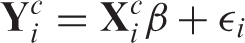
In many longitudinal studies, researchers are often interested in the effect of the predictor Z on the slope or rate of change in the outcome, which can be evaluated in the following model

In model (1), the jth row of the design matrix
In reality, longitudinal data are often unbalanced due to missing data. Denote
Denote q as the number of possible values that
The parameter β = (β0, β1, β2, β3)
T
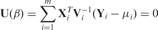
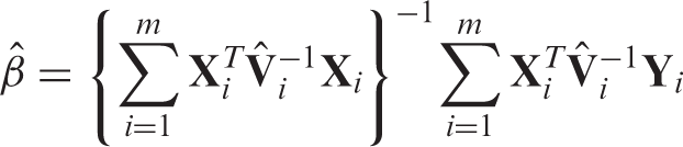
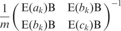
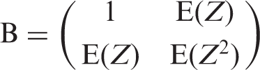
in the linear mixed effects model (1) is estimated by solving the following estimating equation

From the variance expression (2), in which the expectation is taken over the joint distribution of
Given planned observation times t = (t1, … , t
n
), the residual variance–covariance matrix V, the distribution of Z, and the missing data distribution P(

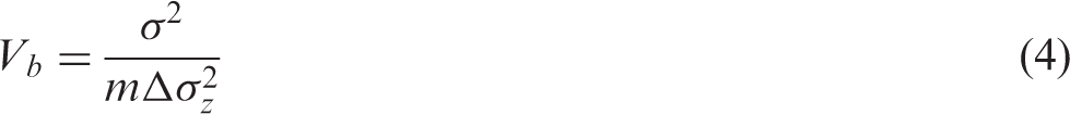
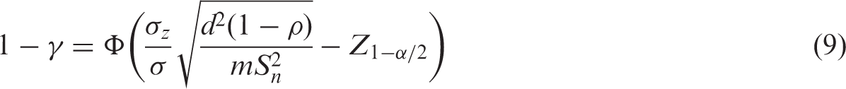
To calculate the sample size m needed or the power 1 − γ for testing the null hypothesis H0: β3 = 0 versus H1: β3 = d using a two-sided α level test, we solve the equation d2 = V b (Z1−α/2 + Z1−γ)2, where Z p is the pth percentile of the standard normal distribution.
We consider the compound symmetry variance structure because it is common and closed form formulae for V b can be easily obtained. We first examine power based on the asymptotic properties of the MLE for the parameter of interest, β3, and evaluate how power depends on the distribution of the missing data in Section 2.2. We then examine two alternative power calculation methods commonly used in practice in Section 2.3. Although we only consider the unadjusted model (1), the methods can be easily extended using the approach of Hsieh et al.36 for controlling for confounders.
2.2 MLE-based method and impact of missing data
2.2.1 MLE-based method for power analysis with missing data
The power for testing β3 in model (1) in the presence of missing data has been studied,22–31 and explicit formulae for sample size and power calculations are available,22–26 but not as a function of the distribution of K for linear mixed effect models. We express the power and sample size formulae in terms of the distribution of K so that it can be more easily compared to the other conventional methods considered here. We assume that the missing data pattern is monotone where the distribution of
Since the inverse of a k × k compound symmetry matrix with variance σ2 and correlation coefficient ρ is
Meanwhile, it can also be shown that δ is far less than the first component of Δ,
When there are no missing data, δ = 0,


If the predictor Z is binary with mean μ
z
, e.g. as in a longitudinal study comparing two treatment groups,
To illustrate how the crucial term Δ in equations (4), (6), and (7) is calculated, we give an example for n = 2. Suppose t = (0, 1) (e.g. t = 0 and 1 indicate baseline and follow-up, respectively), the intraclass correlation coefficient is ρ = 0.5, and the drop out rate at follow-up is 30%, so
2.2.2 Impact of missing data
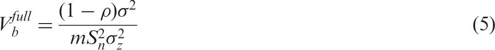
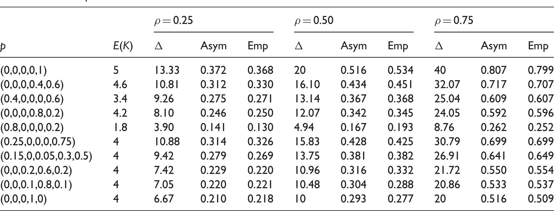
Expressions (4), (6), and (7) suggest that the impact of missing data on the power for testing β3 is through the function Δ, which depends on the maximum number of measurements n, correlation coefficient ρ, the value of time of measurements t, and the distribution
Δ and power for some distributions of K from studies with n = 5.
2.2.3 Adjusting for confounders
To adjust for a set of confounders, W, and the interaction between W and time when examining the effect of the main predictor variable on the slope in model (1), we can follow the method in the study of Hsieh et al.36 and simply replace
2.3 Alternative methods
In practice, alternative approaches that simply modify the complete data formula (8) or (9) are often used.
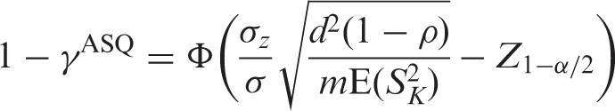
2.3.1 ASQ method
Since the power analysis formulae for complete data, (8) and (9), depend on n only through
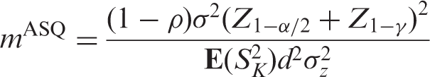
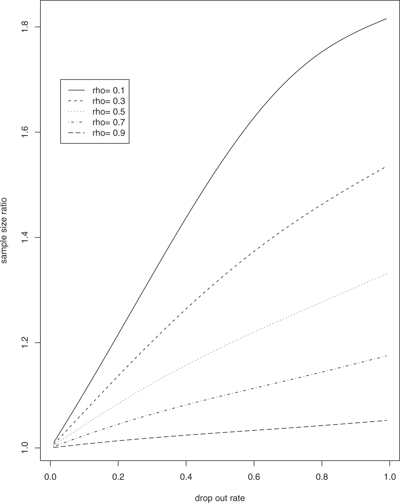
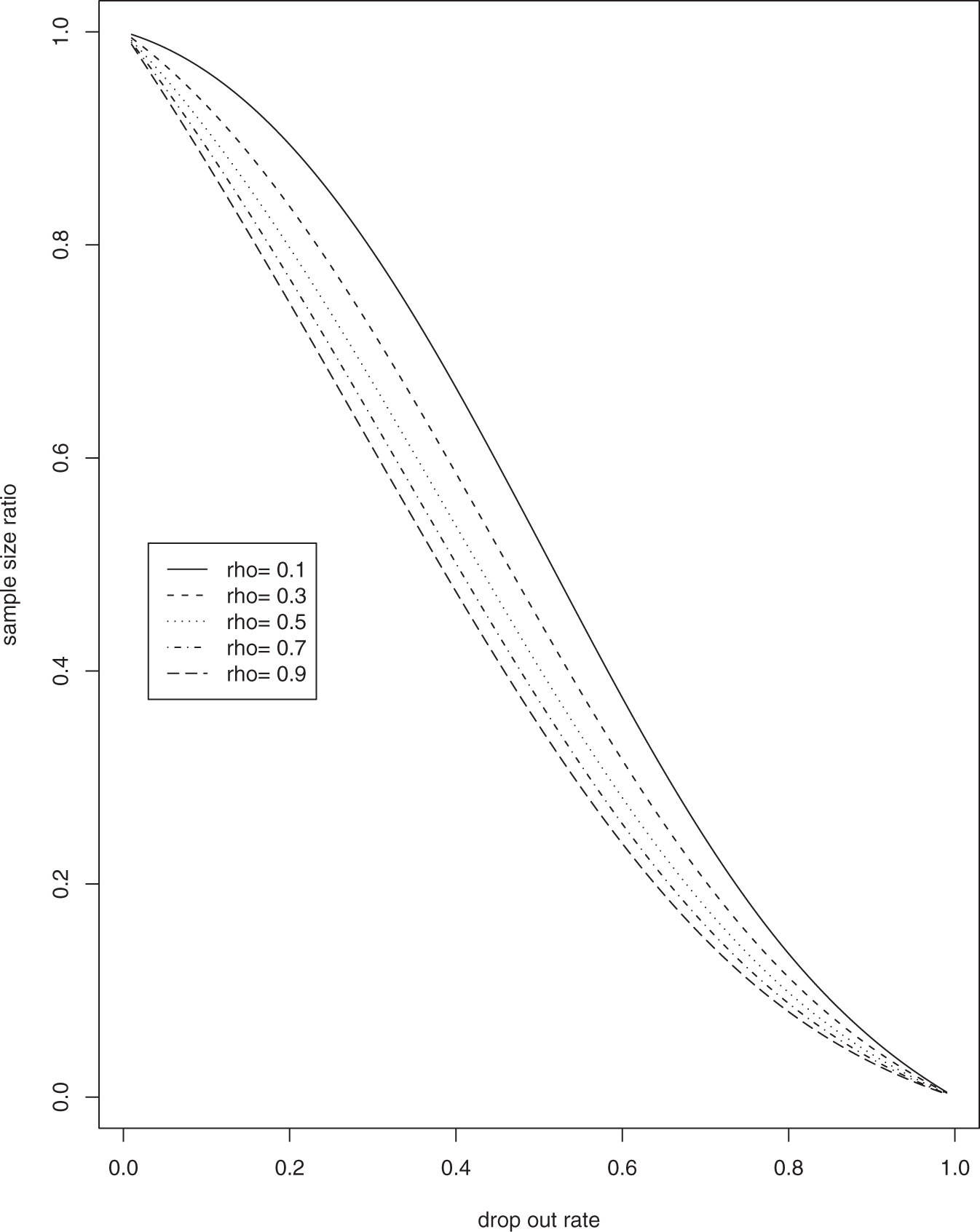
We examined the ratio of the sample size estimates using the ASQ method versus the MLE-based method, mASQ/m, in a longitudinal study with n = 2 and n = 5, various values of the correlation coefficient ρ, and a constant drop out rate. Results are shown in Figures 1 and 2 for n = 2 and n = 5, respectively. The figures show that the ratio mASQ/m is always greater than or equal to 1, increases as ρ decreases or as the drop out rate increases, and increases faster as the drop out increases when the correlation ρ is smaller. As the drop out rate approaches 1, the ratio reaches a limit less than 2 for both n = 2 and n = 5, i.e. ASQ overestimates sample size by no more than 100%. When ρ is large and the drop out rate is moderate or small, the ratio is close to 1, and thus the ASQ method is a good approximation to the MLE-based method. For example, when ρ = 0.8 and the drop out rate is 30% in the case of n = 2, it only overestimates the sample size by about 3%.
Ratio of sample size calculated using the ASQ method versus the MLE-based method for n = 2. ASQ, average sum of squares; MLE, maximum likelihood estimate. Ratio of sample size calculated using the ASQ method versus the MLE-based method for n = 5. ASQ, average sum of squares; MLE, maximum likelihood estimate.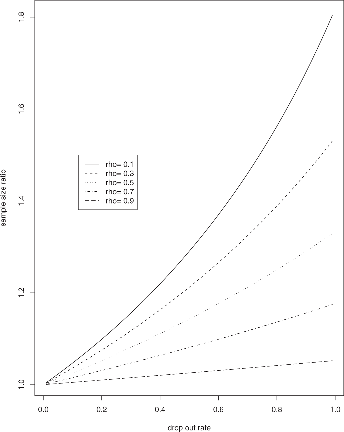
2.3.2 ANS method
Another commonly used approach for computing power with missing data is to equate it to a balanced longitudinal study without missing data that has the same total number of repeated measurements

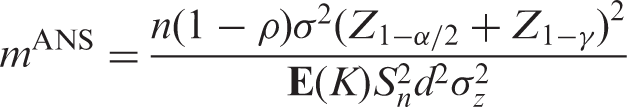
The function
We examined the ratio of the sample size calculated using the ANS method versus the correct method,
Ratio of sample size calculated using the ANS method versus the MLE-based method for n = 2. ANS, average number of subjects; MLE, maximum likelihood estimate. Ratio of sample size calculated using the ANS method versus the MLE-based method for n = 5. ANS, average number of subjects; MLE, maximum likelihood estimate.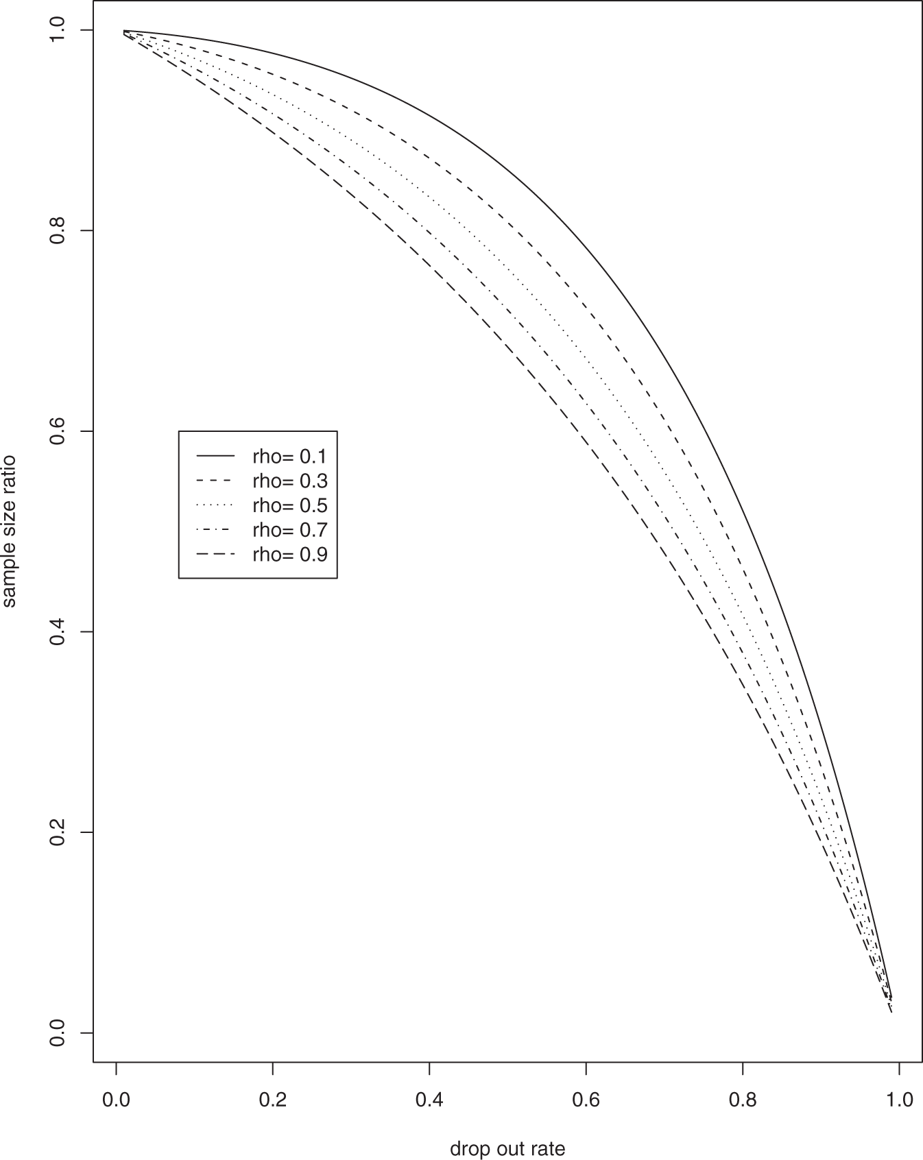
When the sample size m is fixed, the ANS power estimate,
2.3.3 Other methods
Other commonly used methods in practice include using only the subset of subjects with all measurements k = n and then applying the complete data formula. Here, only a proportion p n of the subjects are used, so it clearly is too conservative, especially when p n is small and n is moderate or large. In the case of n = 2, it is equivalent to the ASQ method. As this method has already been studied in the literature,24 we do not consider it further in this article.
3 Simulation studies
3.1 Simulation study 1
In the first simulation study, the missing data were generated completely at random, and our goal was to examine the performance of the MLE-based methods and the conventional ASQ and ANS ones. We considered longitudinal studies with two and five visits, representing short and moderate lengths of follow-up, respectively. For n = 2, the planned follow-up times t = (0, 1), representing baseline and follow-up visits; for n = 5, we have t = (0, 1, 2, 3, 4), representing baseline and four follow-up visits with equal time intervals (e.g. annually). We considered values of 0.25, 0.50, and 0.75 for the correlation coefficient ρ, representing low, medium, and high levels of correlation, respectively. The predictor variable, Z, was generated from a Bernoulli distribution with P(Z = 1) = 0.5 for the case of n = 2, and standard normal for the case of n = 5. The repeatedly measured outcome Y was generated from model (1), with β0 = β1 = β2 = 0, σ2 = 1. The first (or baseline) measure Y1 was observed for every subject. For the missing data distribution, the observation indicator R2 for the follow-up measure Y2 in the case of n = 2 was generated from a Bernoulli distribution with P(R2 = 1|Z, Y1) = 1 − p d . In the case of n = 5, a constant drop out rate p d was considered, with P(R ij = 1|Rij−1 = 1, Z i , Yi1, … , Yij−1) = 1 − p d , j = 2, … , 5. Values of 0.1, 0.2, and 0.3, commonly observed in longitudinal studies, were considered for the drop out rate p d . We evaluated the power for given sample size m of 100, 200, 300, 400, and 500, with β3 = −0.3 and −0.02 for n = 2 and n = 5, respectively. Empirical power estimates from 2000 simulations (Emp) were obtained, and compared to the power estimates using the MLE-based method (Asym), ASQ and ANS methods. Sample size estimates from different methods for given power of 80% and 90% were also examined, with β3 = 0.3 and 0.04 for n = 2 and n = 5, respectively, along with the empirical power estimates from 2000 simulations (Emp) using the estimated sample sizes. Extreme drop out rates of 0.5, 0.7, and 0.9 were also considered. For assessing power estimates, sample sizes of m = 500 for the case of n = 2 and m = 10000 for the case of n = 5 were used. For evaluating sample size estimates for a given power, the target power was set at 80% with β3 = 0.3 and 0.05 for n = 2 and n = 5, respectively. The situation of no missing data was also considered as a reference, in which case all three power analysis methods were reduced to the complete data formulae.
Empirical power from 2000 simulations and power estimates using the MLE-based (Asym), the ASQ and ANS methods under different drop out rate p d , correlations ρ, and sample size m.
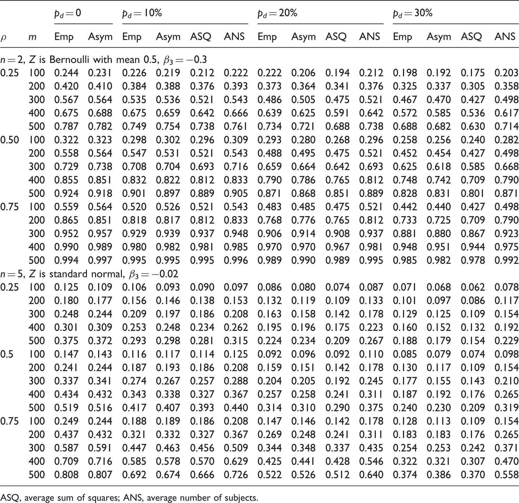
ASQ, average sum of squares; ANS, average number of subjects.
Sample size estimates (empirical power from 2000 simulations) using the MLE-based (Asym), the ASQ and ANS methods under different drop out rates p d , correlations ρ and power.
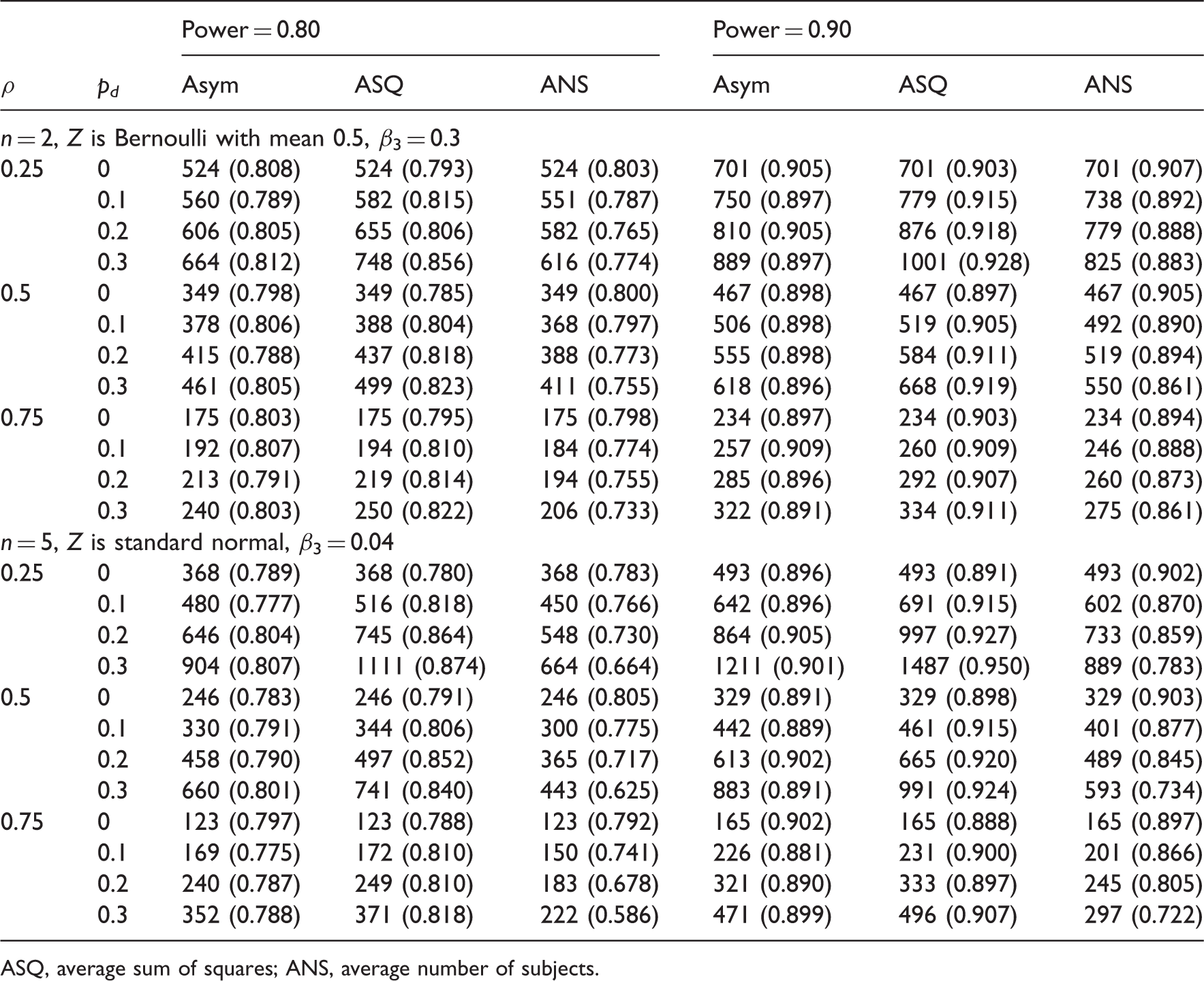
ASQ, average sum of squares; ANS, average number of subjects.
Empirical power from 2000 simulations using the MLE-based (Asym), the ASQ and ANS methods under extremely large constant drop out rate p d .
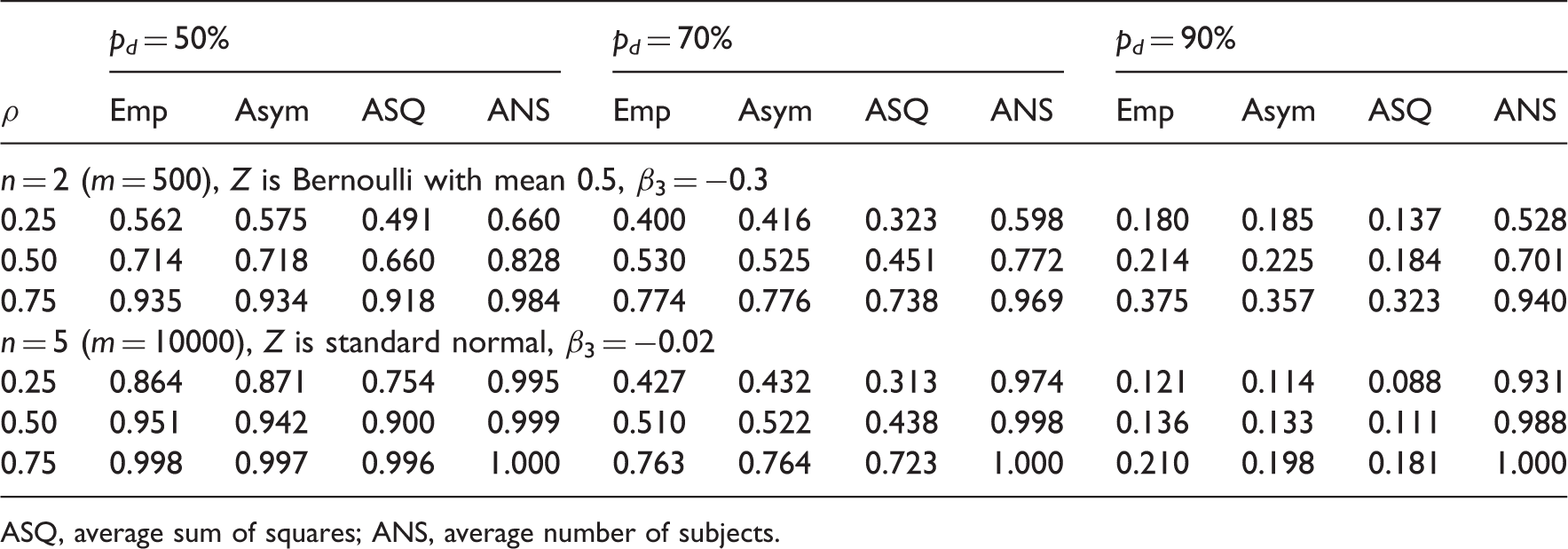
ASQ, average sum of squares; ANS, average number of subjects.
Sample size estimates (empirical power from 2000 simulations) given 80% power using the MLE-based (Asym), the ASQ and ANS methods under extremely large constant drop out rate p d .
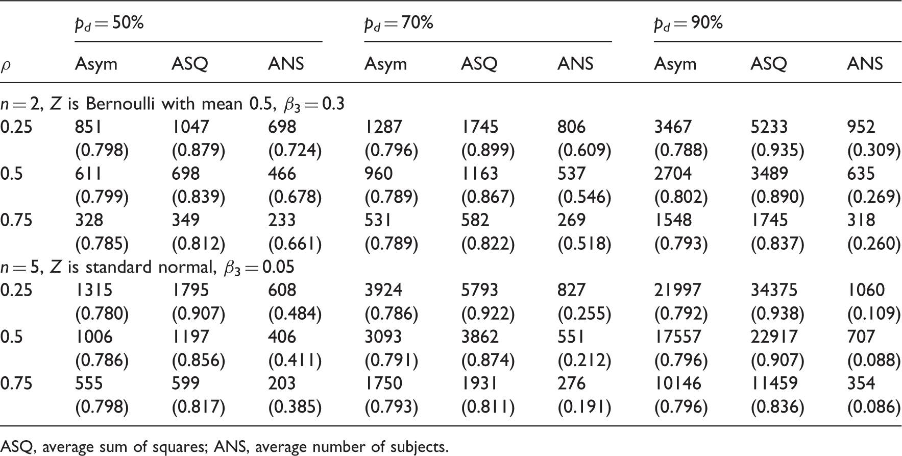
ASQ, average sum of squares; ANS, average number of subjects.
3.2 Simulation study 2
Empirical power from 2000 simulations under different (π1, π2) values when missing data are MAR (n = 2).
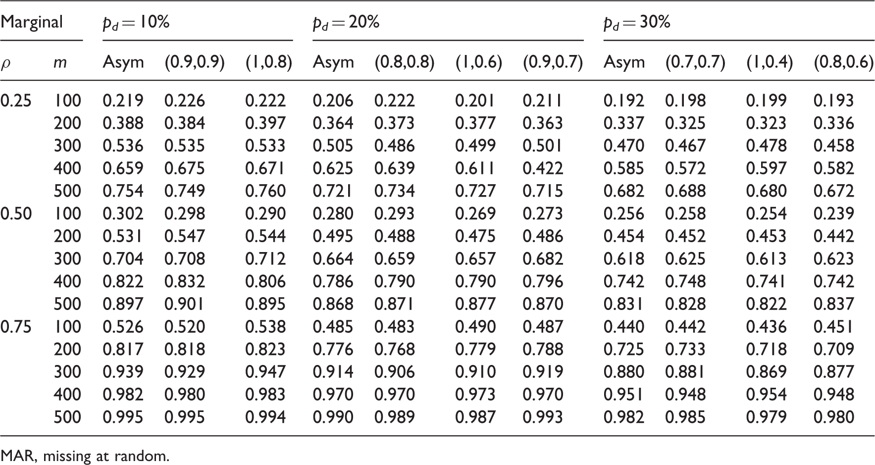
MAR, missing at random.
Empirical power from 2000 simulations under different (π1, π2) values when missing data are MAR (n = 5) (all correspond to marginal distribution p = (0.5, 0, 0, 0, 0.5)).
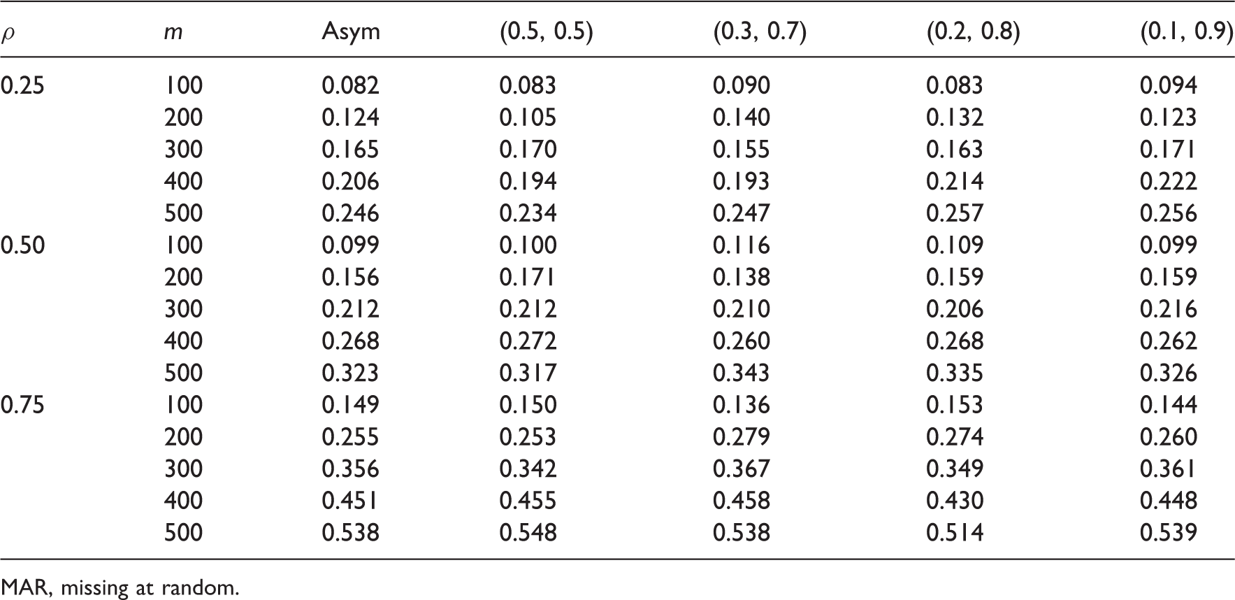
MAR, missing at random.
From Tables 6 and 7, the empirical power estimates from different MAR cases with the same marginal drop out rate are all similar to that from the MCAR case, and all empirical power estimates are similar to the MLE-based power estimates which only used the marginal distribution of the missing data.
4 Examples
We apply the MLE-based method and the ASQ and ANS methods to the power analysis of two longitudinal studies in the elderly. Empirical power estimates from 2000 simulations are also obtained.
4.1 Example 1: Between group comparison of change before and after treatment in a clinical trial with two visits
In designing a randomized clinical trial to test the efficacy of CR in improving mobility in sedentary seniors,37 eligible participants will be randomized equally either to CR or health education control group. The primary mobility outcome is the change in gait velocity from baseline at the end of the intervention. The primary hypothesis is that subjects in the CR intervention group will show better improvement in gait velocity than those in the control group.
The linear mixed effects model (1) will be used to analyze the data. Here, the predictor Z, an indicator of the intervention group, is binary with P(Z i = 1) = 0.5. The goal was to estimate the sample size needed to detect, with 85% power, a difference of 4 cm/s in the change of gait velocity between the intervention and control group, with an expected drop out rate of 20% after intervention.
Based on previous studies,38 the value of σ is assumed to be 24 cm/s and the intraclass correlation coefficient ρ is 0.875. Using formula (6) from the MLE-based method, the estimate of sample size needed is m = 400. Using the ASQ method, the sample size estimate is 406, close to the correct value because ρ is large and the expected drop out is not severe. With the ANS method, the estimated sample size is 360, which underestimates the correct sample size by 10%. Simulation studies with 2000 repetitions were performed to evaluate the empirical power using these sample size estimates. The empirical power from sample sizes of 400, 406, and 360, estimated using the MLE-based, ASQ, and ANS methods, respectively, are 85.2%, 85.1%, and 81.2%. The MLE-based and ASQ sample size estimates are similar, and both yield empirical power estimates similar to the target level of 85%. As expected, the underestimated sample size using the ANS approach results in an empirical power estimate smaller than the target value.
4.2 Example 2: Effect of a continuous predictor on the slope in a longitudinal study with five visits
In designing one of the projects in the renewal application of the EAS,39 a long-term study of aging, it is assumed that 390 subjects with baseline measures of cerebral vascular reactivity would be available. The primary hypothesis is that this variable would be associated with the rate of cognitive decline as measured by Free and Cued Selective Reminding Test (FCSRT).40 The study cohort will consist of a mix of active study participants and new enrollees. The outcome will be measured at baseline and each annual follow-up visit during a 5-year study period. Given the study design and the expected attrition rate, it is projected that 30%, 9%, 24%, 19%, and 18% of the sample will have 1, 2, 3, 4, and 5 repeated measures in FCSRT, respectively; the intraclass correlation ρ is 0.50, and the conditional standard deviation σ is 6.4.
The goal was to determine the power for detecting a difference of 0.35 points per year in the rate of cognitive decline in FCSRT corresponding to a 1 SD unit difference in the cerebral vascular reactivity measure using a two-sided α level 0.05 test and 390 total subjects.
The power estimates are 0.83, 0.79, and 0.95 using the MLE-based, ASQ, and ANS methods, respectively. The empirical power estimate from 2000 simulations is 0.813, close to the MLE-based estimate. The ASQ method slightly underestimated power, while the ANS method overestimated power by 17%.
5 Discussion
Missing data are common in longitudinal studies and therefore should be taken into account when assessing power for testing the effect of a predictor variable on the rate of change in the outcome. Despite the availability of methods for evaluating power with missing data, it has remained unclear how missing data actually affect power, and erroneous approaches are still often used in practice. We have shown that the ASQ method ignores a non-negative component of the Δ function, and thus results in an overestimated sample size or underestimated power, especially when the correlation between repeated measures is small and the proportion of missing data is high. For small to moderate degrees of missing data and large intraclass correlation, the ASQ is similar to the MLE-based approach. The ANS method, on the other hand, assumes that subjects with incomplete and complete data contribute to the power analysis equally, and thus can result in seriously overestimated power or underestimated sample size, especially when the degree of missing data is severe and the number of planned visits and the correlation among repeated measures are moderate or large. Extensive simulation studies have confirmed these conclusions. The power analysis method is based on a linear mixed effects model which assumes that the data are MAR, i.e. the missing data can depend on the observed outcome given the predictor. However, only the marginal distribution of the missing data, i.e. the distribution of missing data given the predictor, is needed for determining power. Our findings suggest that the ANS method can be greatly misleading and should not be used. The conservative ASQ method can be a good approximation when the correlation is large and the extent of missing data is moderate. Based on our simulation studies, the asymptotically correct MLE-based method performs well with limited sample sizes and is recommended especially with large amounts of missing data.
Footnotes
Funding
This study was funded by National Institute of Health [P01-AG03949 and R01-AG02511903].
Conflict of interest
None declared.