Analysis of cross-over studies with missing data

Abstract

This paper addresses some aspects of the analysis of cross-over trials with missing or incomplete data. A literature review on the topic reveals that many proposals provide correct results under the missing completely at random assumption while only some consider the more general missing at random situation. It is argued that mixed-effects models have a role in this context to recover some of the missing intra-subject from the inter-subject information, in particular when missingness is ignorable. Eventually, sensitivity analyses to deal with more general missingness mechanisms are presented.

Keywords

cross-over trials fixed-effects model mixed-effects model missing data sensitivity analyses

1 Introduction

The issue of missing data in clinical trials is almost ubiquitous. While this is well recognized for adequate and well-controlled trials and to some extent addressed by regulatory guidelines,¹ it seems to be less recognized for trials in early drug development. During that development phase pharmacokinetic studies play a role as first in man, bioequivalence (BE), drug–drug interaction (DDI), or food interaction studies which frequently apply a cross-over design. The complete case (CC) analysis as proposed by Grizzle² that considers only subjects that completed the entire sequence of periods is often still considered the benchmark method despite its proneness for biased results.

An early reference on the analysis of incomplete data in a two-period cross-over design is Patel’s³ paper. This paper suggests a maximum-likelihood estimator under the assumption of missingness in period 2 only. No restrictions on the variances of the response variable in different periods or under different treatments are made. Kenward and Molenberghs⁴ pointed out that Patel’s method could not be applied in a missing at random (MAR) situation because his precision estimator is based on a missing completely at random (MCAR) framework. Lee et al.⁵ modified the method to provide correct estimates under MAR. (A definition of the different missingness mechanisms are provided in Section 2.)

Some authors focused attention on three-period two-treatment cross-over designs to be able to estimate carry-over effects which is not possible in 2 × 2 cross-over studies. Richardson and Flack⁶ studied maximum-likelihood estimators and imputation methods for these designs and compared them with CC analyses. Chow and Shao⁷ developed an analysis method that is applicable to a design where two treatments are administered in sequences of three periods such that each subject completes at least two out of three periods. For their approach no assumptions on the distribution of the random effects in the common mixed-effects analysis model are required. It is not explicitly mentioned under which mechanism of missingness their analysis provides correct results. In fact, their estimator is a special case of the standard least-squares estimator (see Jones and Kenward,⁸ p. 9), and hence the method described in Chow and Shao⁷ would account for MCAR only.

None of the papers cited so far did consider the missing not at random (MNAR) situation which is not unlikely to happen. Richardson and Flack⁶ examined to what extent the maximum-likelihood estimator fails under these circumstances. A recent paper by Basu and Santra⁹ describes a model that includes the measurement and an outcome-dependent dropout process. However, their proposal looks like a Bayesian version of the Diggle and Kenward¹⁰ approach. This paper attempted to estimate parameters from an informative missingness model to obtain evidence for MNAR. It also contains a simulation on the impact of MNAR on the analyses of a 4 × 4 cross-over trial with a Williams square design.

Since cross-over studies play a prominent role in drug development, for example, in BE trials, regulatory guidelines exist that propose analysis methods for these trials. The guideline made effective by CHMP¹¹ in 2010 states the following: “The pharmacokinetic parameters under consideration should be analyzed using ANOVA … The statistical analysis should take into account sources of variation that can be reasonably assumed to have an effect on the response variable. The terms to be used in the ANOVA model are usually sequence, subject within sequence, period and formulation. Fixed effects, rather than random effects, should be used for all terms.”

The respective FDA guideline¹² recommends “For non-replicated crossover designs, this guidance recommends parametric (normal-theory) procedures to analyze log-transformed BA [bioavailability] measures. General linear model procedures available in PROC GLM in SAS or equivalent software are preferred, although linear mixed-effects model procedures can also be indicated for analysis of nonreplicated crossover studies. For example, for a conventional two-treatment, two-period, two-sequence (2 × 2) randomized crossover design, the statistical model typically includes factors accounting for the following sources of variation: sequence, subjects nested in sequences, period, and treatment … Linear mixed-effects model procedures, available in PROC MIXED in SAS or equivalent software, should be used for the analysis of replicated crossover studies for average BE.”

The CHMP guideline does not touch on the issue of missing observations at all. The FDA guideline does so only in the context of individual BE, but not for the concept of average BE which is applied most often in practice. To close this gap, this paper investigates the different approaches to cross-over trials in the context of incomplete data. The next section contains a review of the fundamental definitions of the missing data mechanisms and a statistical model for cross-over studies. In Section 3, we re-analyze the data from Chow and Shao⁷ using fixed and mixed models and provide some simulations for the single sequence cross-over trial with incomplete data. Section 4 presents sensitivity analyses for the Chow and Shao⁷ data.

2 Statistical background

2.1 Missingness mechanisms

In the following, we shortly review Rubin’s¹³ taxonomy of missing data mechanisms. Let Y represent the complete set of measurements on a unit or subject and R the associated missing value indicator. For a realization of (y, r) the elements of r take the values 1 and 0 indicating, respectively, whether the corresponding elements of y are observed or not. Let $(y_{o}, y_{m})$ denote the partition of y into the respective sets of observed and missing data. The joint probability density function of Y and R is denoted by $f (y, r | θ, η)$ . If the parameters describing the measurement process (θ) are functionally independent of those describing the missingness process (η) this joint distribution can be represented in the selection model factorization

f (y, r | θ, η) = f (y | θ) ⪻ [R = r | y, η]

(1)

Alternatively, a pattern mixture model factorization can be obtained

f (y, r | φ, ψ) = f (y | r, φ) ⪻ [R = r | ψ]

(2)

Note that (θ, η) has been replaced with $(φ, ψ)$ in (2) since the parameters of the two factorizations may differ. For a selection model, the marginal distribution of the data $f (y | θ)$ and the conditional distribution of the missingness mechanism given the data are to be specified. The pattern mixture model focuses on the conditional distribution of the data given a missingness pattern r. This allows to specify a different distribution $f (y | φ (r))$ for each pattern. The marginal distribution of Y is then given as a mixture of the conditional distributions

f (y | θ) = \sum_{r} f (y | φ (r)) ⪻ [R = r | ψ]

On the other hand, if the marginal distribution of Y and the conditional distribution of R given Y are known, the conditional distribution of Y given r follows from (1) and (2)

f (y | φ (r)) = f (y | θ) \frac{⪻ [R = r | y, η]}{⪻ [R = r | ψ]}

(3)

with

⪻ [R = r | ψ] = \int f (y | θ) ⪻ [R = r | y, η] d y

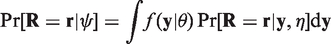
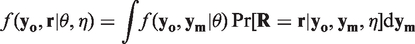
One obtains the distribution of the observed values by integrating out the missing observations. Doing this for the selection model (1) leads to

f (y_{o}, r | θ, η) = \int f (y_{o}, y_{m} | θ) ⪻ [R = r | y_{o}, y_{m}, η] d y_{m}

Under the MCAR mechanism the probability of an observation being missing is independent of the responses

⪻ [R = r | y, η] = ⪻ [R = r | η]

This implies

f (y_{o}, r | θ, η) = ⪻ [R = r | η] \int f (y_{o}, y_{m} | θ) d y_{m} = f (y_{o} | θ) ⪻ [R = r | η]

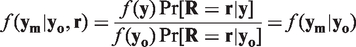
It follows from (3) that MCAR holds when all conditional distributions of the measurements given the missingness patterns are equal to the marginal distribution of the measurements and vice versa. In this case, selection and pattern mixture models are identical, that is, $θ = φ$ and $η = ψ$ .

For MAR the probability of missing depends only on observed data, that is

⪻ [R = r | y, η] = ⪻ [R = r | y_{o}, η]

Here, we obtain

f (y_{o}, r | θ, η) = ⪻ [R = r | y_{o}, η] \int f (y_{o}, y_{m} | θ) d y_{m} = f (y_{o} | θ) ⪻ [R = r | y_{o}, η]

A straightforward consequence of MAR is that the conditional distribution of the missing observations given the observed measurements does not depend on the missingness pattern

f (y_{m} | y_{o}, r) = \frac{f (y) ⪻ [R = r | y]}{f (y_{o}) ⪻ [R = r | y_{o}]} = f (y_{m} | y_{o})

For both MCAR and MAR, inference can be based on the observed portion of the data, while the missingness mechanism can be ignored. Under this condition, likelihood-based analyses on the observed data are providing valid results when the caveats described in Kenward and Molenberghs⁴ and Kenward¹³ are considered. Particularly for MCAR, the analysis could be based on those units with complete information (CC analysis) since the missingness mechanism provides an independent random selection, although such an analysis would be inefficient.

When none of the above criteria holds then MNAR applies. In this case, the distribution of the missing data given the observed data and the missingness mechanism needs to be known for valid inferences, and both θ and η have to be estimable from the data

f (y_{o}, r | θ, η) = \int f (y_{o}, y_{m} | θ) ⪻ [R = r | y_{o}, y_{m}, η] d y_{m} = f (y_{o} | θ) \int f (y_{m} | y_{o}, θ) ⪻ [R = r | y_{o}, y_{m}, η] d y_{m}

As in many other situations, assumptions have to be made on the distributions involved. However, in the MNAR situation these assumptions are principally not verifiable for all data, but only for the observed data. The best achievable is to analyze the data under a range of plausible alternative assumptions and to investigate the robustness of the results under these alternatives. An instructive example of a data-driven sensitivity analysis in the context of a selection model is Kenward.¹⁴ Molenberghs et al.¹⁵ considered a formal way of conducting sensitivity analyses by introducing influence analysis.

2.2 Cross-over studies

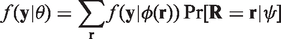
We consider general cross-over designs with p periods and t treatments. Let Y_ij denote the observation from subject i at period j. We model Y_ij as

Y_{ij} = μ + U_{ij} + π_{j} + τ_{(i, j)} + e_{ij}

(4)

where

π_{j}

denotes the effect of period j, τ_(i,j) is the treatment effect at the j-th period of i-th individual, and U_ij is a subject specific random effect independently distributed from the random errors e_ij.

It should be noted that in contrast to the recommendations in guidelines we do not account for a sequence effect for several reasons. First, for fixed-subject effects, a sequence effect would just confound the subject effect such that subject within sequence would have to be included into the model to render the sequence effect estimable. For random-subject effects, the inclusion of a sequence effect is discouraged, because this would be essentially self-contradictory: random effects are included to allow the incorporation of between-subject information on the mean effects, while fixed-sequence effects remove this information (see Kenward and Roger¹⁶). Last and most importantly, subjects are randomly assigned to sequences and therefore by design the expected sequence effect is zero.

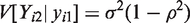
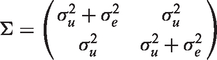
The random-subject effects are assumed to be identically and independently normally distributed with zero mean and covariance matrix Λ while the random errors are assumed to follow a normal distribution with zero mean and covariance matrix Δ not otherwise specified. Then the covariance matrix of the vector of observations from the i-th subject, $y_{i} = (y_{i 1}, \dots, y_{ip})$ , is given by

Σ = Δ + Λ

In the special case of the same random effect for all periods, that is, when subject is the only random effect in the model, u_ij = u_i holds for all j. With $V (u_{i}) = σ_{u}^{2}$ one obtains

Λ = σ_{u}^{2} J_{p}

(5)

where J_p is a p × p-dimensional matrix of ones. This constitutes the most relevant case for cross-over studies. Similarly, if the e_ij are assumed to be independent with variance

σ_{e}^{2}

, then

Δ = σ_{e}^{2} I_{p}

(6)

where I_p denotes the p-dimensional identity matrix. When both of these special cases hold, Σ has a compound symmetry structure.

Parameter estimates are usually obtained from restricted maximum-likelihood estimation which allows to estimate the parameters of Σ in an unbiased way without having to estimate the fixed effects such as period or treatment effect first. Since the fixed effects are estimated given estimates of the variance parameters, their variability can be underestimated if the variability of the latter is not taken into consideration.

3 Mixed- versus fixed-effect models

3.1 Data from Chow and Shao

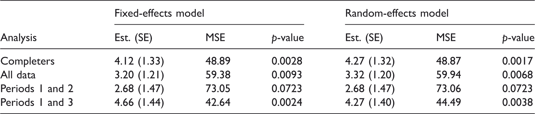
Here, we analyze the data presented in Chow and Shao,⁷ which have been re-analyzed in Basu and Santra.⁹ These data stem from a two-treatment, 3-period cross-over design where the treatment of period 2 in each of two sequences is repeated in period 3. Thirty-two patients were randomized into the first sequence and 34 into the second sequence. Missing data occurred only in period 3, namely, 8 for sequence 1 and 18 for sequence 2.

We run six different analyses for this data set based on model (4) with covariances (5) and (6) for the random effect and the random error, respectively. First, we consider completers only, that is, all patients with complete data from three periods, thereby reducing the total sample size from 68 to 42. In a second analysis, we consider only data from the first two periods to obtain 68 completers. Admittedly, nobody would add a third period to a cross-over trial and then ignore the data of that period entirely because some of them are missing, but this is done for illustrative purposes only. The third analysis considers all data obtained. We assume that there is no carry-over effect.

The results are obtained using a fixed-effects model (with treatment, period, and patient) and a mixed model (with sequence and treatment as fixed and patient as a random effect).

The mixed-effects analysis used the variance estimates and degrees of freedom as proposed in Kenward and Roger¹⁷ and implemented in PROC MIXED of SAS.¹⁸ With this option the software applies the observed information matrix as proposed in Kenward and Molenberghs.⁴ The results are shown in Table 1. In this example, there is not much of a difference between the analysis based on a fixed or a random-effects model. For the data set comprising periods 1 and 2 only, the results are identical, for the others there is a small difference. However, the biggest difference stems from excluding different parts of the data set from the analysis. Taking data from all periods into consideration, the completer analysis provides a larger treatment effect than an analysis using all available data. The smallest estimator stems from the analysis considering only the first two periods (with a loss of significance) while the analysis including periods 1 and 3 only again provides a large effect estimator.

Table 1.

Estimates with standard errors, mean square errors (MSE), and p-values from different analyses of the Chow and Shao data.

Fixed-effects model			Random-effects model
Analysis	Est. (SE)	MSE	p-value	Est. (SE)	MSE	p-value
Completers	4.12 (1.33)	48.89	0.0028	4.27 (1.32)	48.87	0.0017
All data	3.20 (1.21)	59.38	0.0093	3.32 (1.20)	59.94	0.0068
Periods 1 and 2	2.68 (1.47)	73.05	0.0723	2.68 (1.47)	73.06	0.0723
Periods 1 and 3	4.66 (1.44)	42.64	0.0024	4.27 (1.40)	44.49	0.0038

3.2 Simulation of a single sequence cross-over trial

A design that is fairly often used to address the question of a potential DDI is the single sequence cross-over trial. Subjects receive drug A during period 1 and drug A and drug B during period 2 to assess the potential change in pharmacokinetics parameters of A in the presence of B. Note that carry-over effects are not an issue in these studies.

To investigate this situation we simulated bivariate normal data (Y_i1, Y_i2) with mean μ = (0, 1), variances σ² = 1 and correlation ρ = 0.5. We assumed no missing data in period 1, but a dropout probability of 0.5 for the period 2 under different missingness mechanisms. If p_i denotes the probability of subject i to dropout after period 1, we set p_i = 0.5 for all subjects for the simulation under MCAR. For MAR missingness, we set

p_{i} = Φ (Y_{i 1})

and for MNAR we set

p_{i} = Φ (Y_{i 2} - 1)

. Here, Φ denotes the cumulative distribution function of a standard normal variable. We then draw a uniformly distributed variable V_i and set Y_i2 to missing if

V_{i} < p_{i}

. We analyzed the completers only and all available data with a fixed-effects model and a mixed-effects model where subject was treated as a random effect in the latter analysis. The results are shown in Table 2.

Table 2.

Results from 10,000 simulations of a single sequence trial (see text for details).

Analysis	Missingness	Complete cases		All data
model	mechanism	Estimate	SE	Estimate	SE
Fixed effects	MCAR	1.0014	0.2022	1.0014	0.2022
	MAR	1.2816	0.1931	1.2816	0.1931
	MNAR	0.7169	0.1921	0.7169	0.1921
Mixed effects	MCAR	1.0014	0.2022	1.0008	0.1887
	MAR	1.2816	0.1931	0.9935	0.2138
	MNAR	0.7169	0.1921	0.5657	0.2630

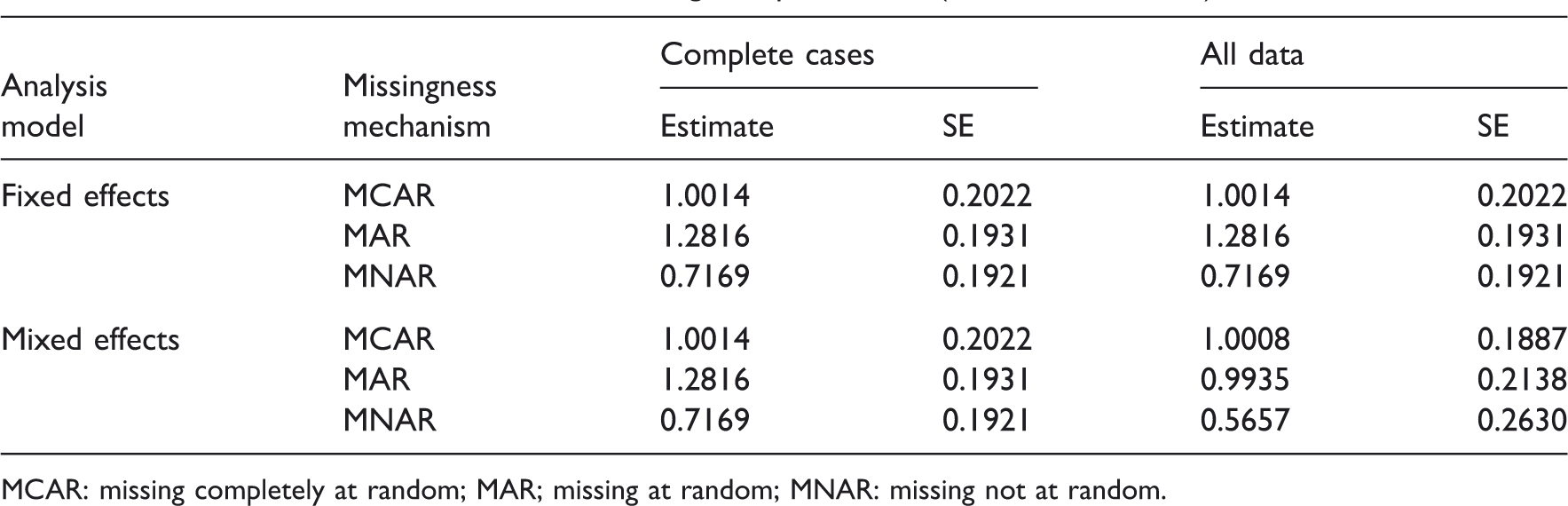
MCAR: missing completely at random; MAR; missing at random; MNAR: missing not at random.

As expected, all analyses fail to provide correct results under MNAR. The results for the fixed-effects model for CCs and all data are the same since the fixed-effects model cannot make use of the information from period 1 when data for the second are missing. The results are also the same as for the random-effects model for CCs since in this case the random effects are canceling out when the contrasts between treatments are formed. The mixed-effects analysis provides on average the correct estimates under MAR when all data are used and under MCAR when all data or just completers are considered. When one uses all data under MCAR, the standard error of the effect estimator is somewhat smaller than without using all the available data. The fixed-effects analysis provides sensible results only under MCAR and overestimates the effect under MAR.

These results call for a clarification of the statement that likelihood-based methods provide valid analyses under MAR. Both fixed-effects and mixed-effect models are likelihood based but only mixed-effects models provided the correct answer in the simulation above. In contrast to the mixed model, the fixed-effects model in the example above cannot use the information from the data of period 1 that predicted the missingness in period 2. Thus, a necessary condition (among others) for a likelihood-based method to provide correct results under MAR is that it utilizes all data points that predict missingness.

4 MNAR analyses based on the selection model

The previous sections have shown that there is a role for mixed-effect models in the analysis of cross-over trials, particularly in the presence of incomplete observations. In the latter case, mixed-effect models provide unbiased estimators of a treatment effect under MAR when the measurement model is correctly specified. However, though the MAR assumption may be reasonable in some cases it does not generally apply.

Under MNAR one needs to model the missingness process as well, not just the measurement process. It is tempting to fit such a model and let the data decide as to whether it fits better than a MAR model. However, such an approach ignores that a goodness-of-fit criterion can only assess the fit of the model to the observed data. Thus, evidence for or against MNAR can be provided solely within a particular predefined parametric family. In fact, every MNAR model can be doubled up with a uniquely defined MAR counterpart that depends on the same parameters and produces exactly the same fit as the original MNAR model.¹⁹

4.1 The single sequence trial

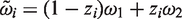
We start with developing sensitivity analyses for the simplest case, that is, bivariate normal data (Y_i1,Y_i2) with mean $μ = (μ_{1}, μ_{2})'$ , variances σ², and correlation ρ. We assume no dropouts during period 1, and that the missingness mechanism follows a logistic model. Let R_i = 1 if period 2 has a measurement and 0 otherwise. Then

logit ⪻ [R_{i} = 1 | y_{i}] = α + β y_{i 1} + ω y_{i 2}

The parameter α reflects the extent of MCAR, β the extent of MAR, and ω the extent of MNAR in the missingness process. In particular, ω = 0 would imply that the missingness mechanism is ignorable. As said above, there is no intention to estimate ω from the data, but to vary it over a range of values to study the impact of MNAR on the estimation of the parameters of interest.

Let $θ = (μ, σ, ρ)$ be the parameter vector of the measurement process and η = (α, β) be the parameter vector of the missingness process. With $g_{ω} (y_{i} | η) = ⪻ [R_{i} = 1]$ , the likelihood of a complete sequence is then given by

L_{ω} (θ, η | y_{i 1}, y_{i 2}) = f (y_{i 1}, y_{i 2} | θ) g_{ω} (y_{i 1}, y_{i 2} | η)

and for an incomplete sequence by

L_{ω} (θ, η | y_{i 1}) = f (y_{i 1} | θ) \int f (y_{i 2} | y_{i 1}, θ) [1 - g_{ω} (y_{i 1}, y_{i 2} | η)] {dy}_{i 2}

Note that $f (y_{i 2} | y_{i 1}, θ)$ is the probability density function of a normally distributed variable with mean

E [Y_{i 2} | y_{i 1}] = μ_{2} + ρ (y_{i 1} - μ_{1})

and variance

V [Y_{i 2} | y_{i 1}] = σ^{2} (1 - ρ^{2})

The likelihood is therefore given by

l_{ω} (θ, η | y_{0}, r) = \sum r_{i} \log L_{ω} (θ, η | y_{i 1}, y_{i 2}) + (1 - r_{i}) \log L_{ω} (θ, η | y_{i 1})

(7)

Sensitivity analyses can then be performed by obtaining parameter estimates of (θ,η) from maximizing (7) for different values of ω.

As an example we conducted such an analysis using the data from periods 2 and 3 of the Chow and Shao data set. Although the same treatments were applied during these periods within each sequence and therefore a zero difference should be expected, separate analyses were performed for the two sequences since the missingness mechanism could be treatment dependent. PROC NLMIXED of SAS¹⁸ was used for the calculations since this software approximates the integrals in the missing data likelihood efficiently by adaptive Gauss–Hermite quadrature (see Liu and Pierce²⁰). A graphical output of the analysis is depicted in Figures 1 and 2.

Figure 1.

Estimates and 95% confidence intervals of the treatment differences $μ_{2} - μ_{1}$ between periods 2 and 3 of the Chow–Shao data set for $- 0.5 \leq ω \leq 0.5$ .

Figure 2.

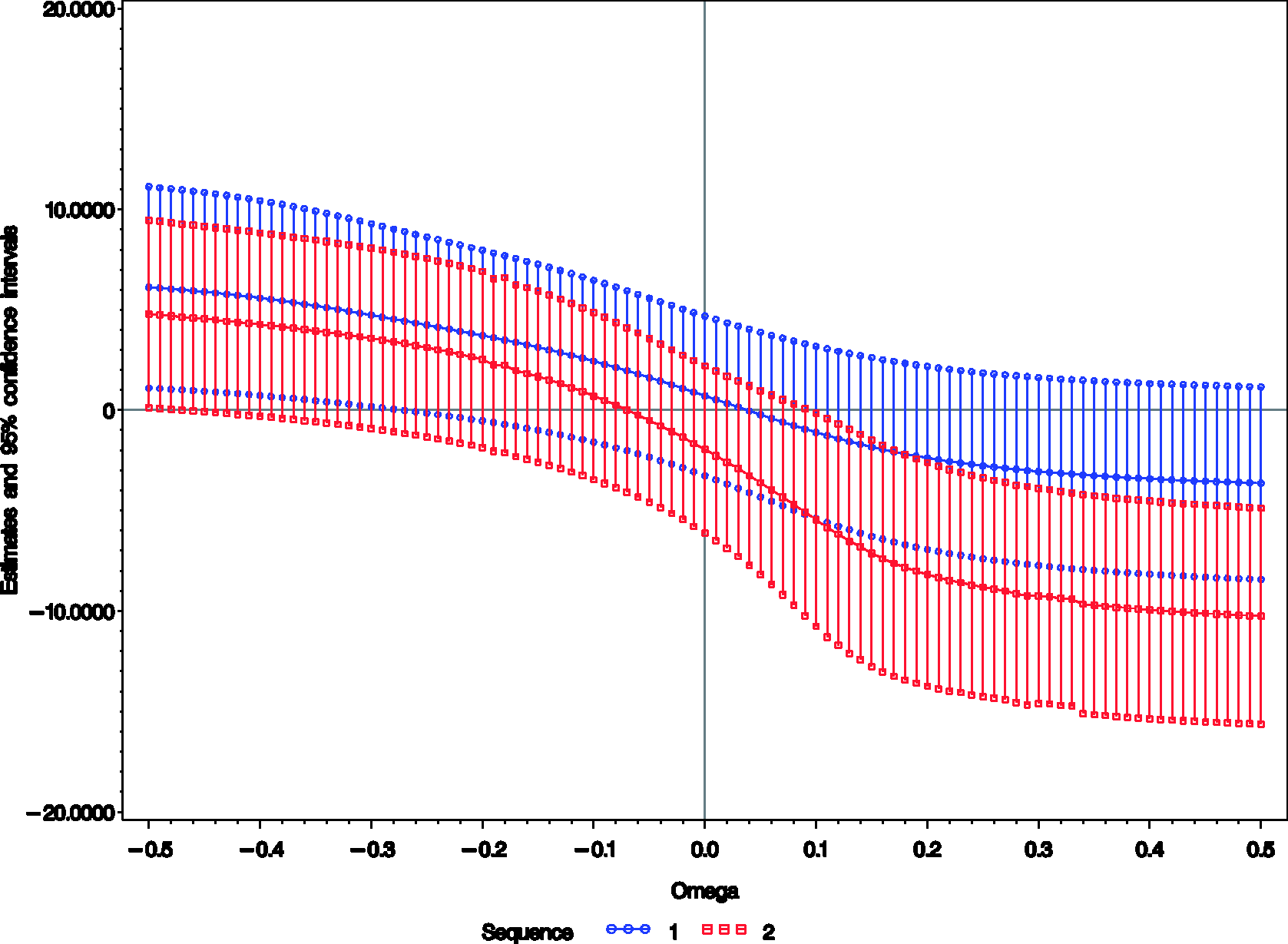
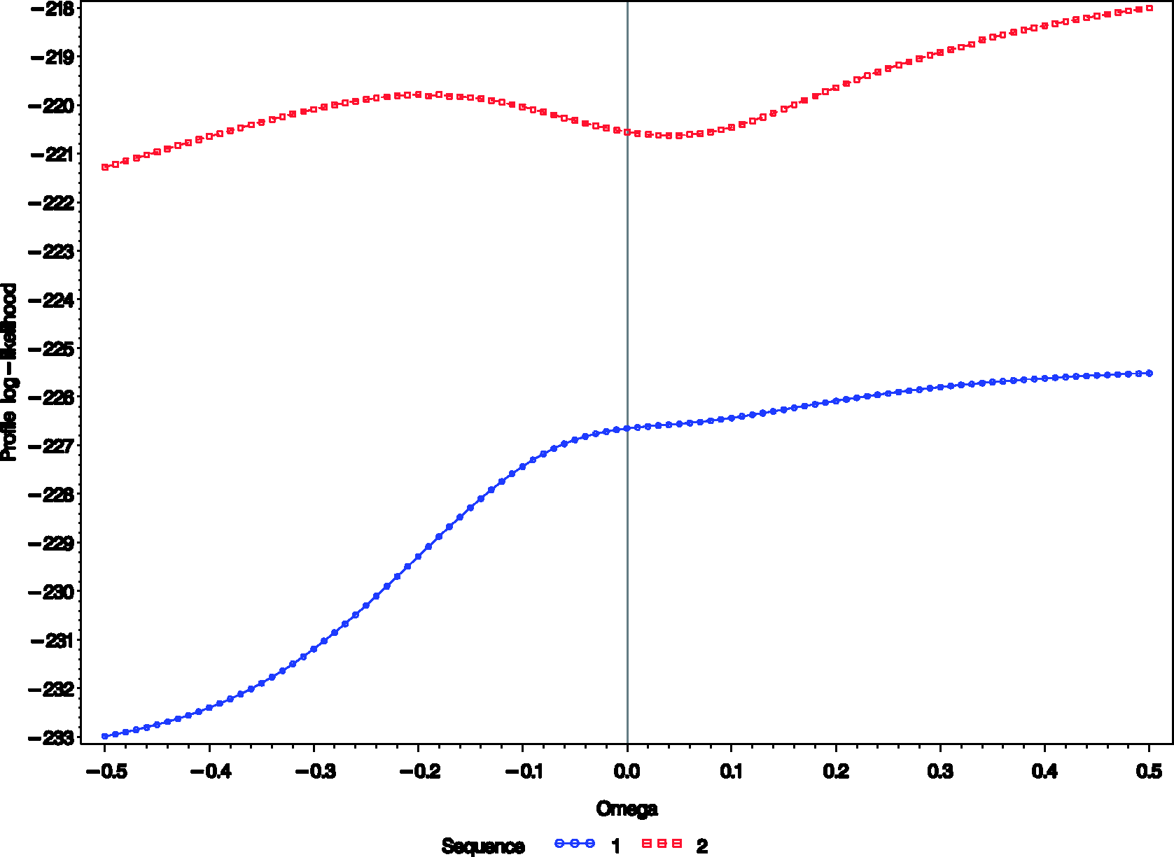
Profile log-likelihood from periods 2 and 3 of the Chow–Shao data set for $- 0.5 \leq ω \leq 0.5$ .

The treatment estimator for the second sequence seems to be more sensitive to MNAR than for the first, particularly for $ω > 0$ . Since we know that the effect should be zero, this behavior indicates that a high degree of MNAR is not a plausible assumption for this data set. Admittedly this kind of consistency check is not available in the common situation where different treatments are studied. For $ω < 0$ , the profile likelihood is decreasing substantially for sequence 1 but is only marginally increasing for $ω > 0$ . For sequence 2, the likelihood is increasing for $ω > 0$ and has a local maximum for $ω \approx - 0.2$ . Would ω have been treated like a parameter to be estimated from a model, the algorithm would likely have found this local maximum close to zero and suggested that the corresponding value of ω describes the extent of MNAR.

4.2 The 2 × 2 cross-over trial

The considerations above can be easily generalized to cover the 2 × 2 cross-over design. Recalling the definitions in Section 2, we have

E [Y_{ij}] = μ_{ij} = μ + π_{j} + τ_{(i, j)}

and

Σ = (σ_{u}^{2} + σ_{e}^{2} σ_{u}^{2} σ_{u}^{2} σ_{u}^{2} + σ_{e}^{2})

and therefore

ρ = σ_{u}^{2} / (σ_{e}^{2} + σ_{u}^{2})

The equation for the mean implies that the distribution of $Y_{i}$ depends on the sequence subject i was assigned to. Assume that treatment τ₁ is administered in period 1 of sequence 1 and period 2 of sequence 2, while τ₂ is administered at period 1 of sequence 2 and period 2 of sequence 1. We introduce a sequence indicator z_i such that z_i = 1 if subject i is assigned to sequence 2 and zero otherwise. The period means can then be written as

μ_{i 1} = μ + π_{1} + (1 - z_{i}) τ_{1} + z_{i} τ_{2}

μ_{i 2} = μ + π_{2} + (1 - z_{i}) τ_{2} + z_{i} τ_{1}

and the dropout mechanism will be modeled as

logit ⪻ [R_{i} = 1 | y_{i}, z_{i}] = α + β y_{i 1} + γ z_{i} + {\tilde{ω}}_{i} y_{i 2}

where the sensitivity parameter is assumed to be treatment dependent by setting

{\tilde{ω}}_{i} = (1 - z_{i}) ω_{1} + z_{i} ω_{2}

With $θ = (μ, π_{1}, π_{2}, τ_{1}, τ_{2}, σ_{u}, σ_{e}), η = (α, β, γ)$ and the sensitivity parameter ω = (ω₁,ω₂), the likelihood of a complete sequence is

L_{ω} (θ, η | y_{i 1}, y_{i 2}) = f (y_{i 1}, y_{i 2} | z_{i}, θ) g_{ω} (y_{i 1}, y_{i 2} | z_{i}, η)

For an incomplete sequence we obtain

L_{ω} (θ, η | y_{i 1}) = f (y_{i 1} | z_{i}, θ) \int f (y_{i 2} | y_{i 1}, z_{i}, θ) [1 - g_{ω} (y_{i 1}, y_{i 2} | z_{i}, η)] {dy}_{i 2}

Note that $f (y_{i 2} | y_{i 1}, z_{i}, θ)$ is the probability density function of a normally distributed variable with mean

E [Y_{i 2} | y_{i 1}, z_{i}] = μ_{i 2} + ρ (y_{i 1} - μ_{i 1})

and variance

V [Y_{i 2} | y_{i 1}, z_{i}] = (σ_{e}^{2} + σ_{u}^{2}) (1 - ρ^{2})

The full likelihood has then the same form as in equation (7).

The results of the sensitivity analysis for periods 1 and 3 data of the Chow and Shao data set are presented in Figures 3 and 4. For ω = 0, the estimate and the standard error for $τ_{2} - τ_{1}$ are 4.2744 and 1.3605, respectively. These values are very close to the estimates obtained from the mixed-model analysis of periods 1 and 3 from the last row and the right column of Table 1.

Figure 3.

Contour plot of the estimates of the treatment differences $τ_{2} - τ_{1}$ between periods 1 and 3 of the Chow–Shao data set ( $- 0.5 \leq ω_{i} \leq 0.5$ ).

Figure 4.

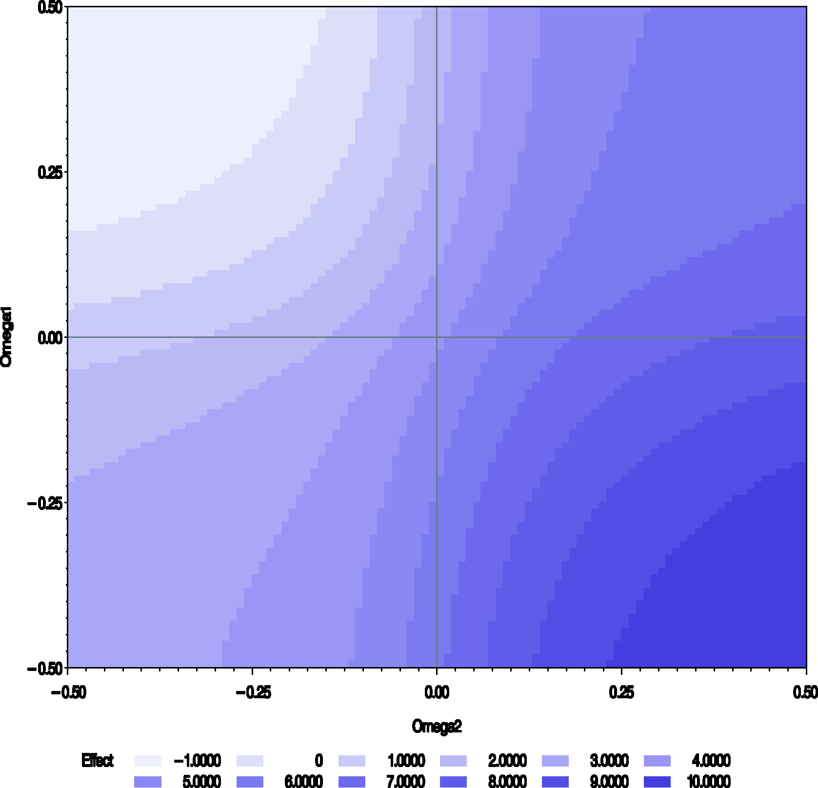
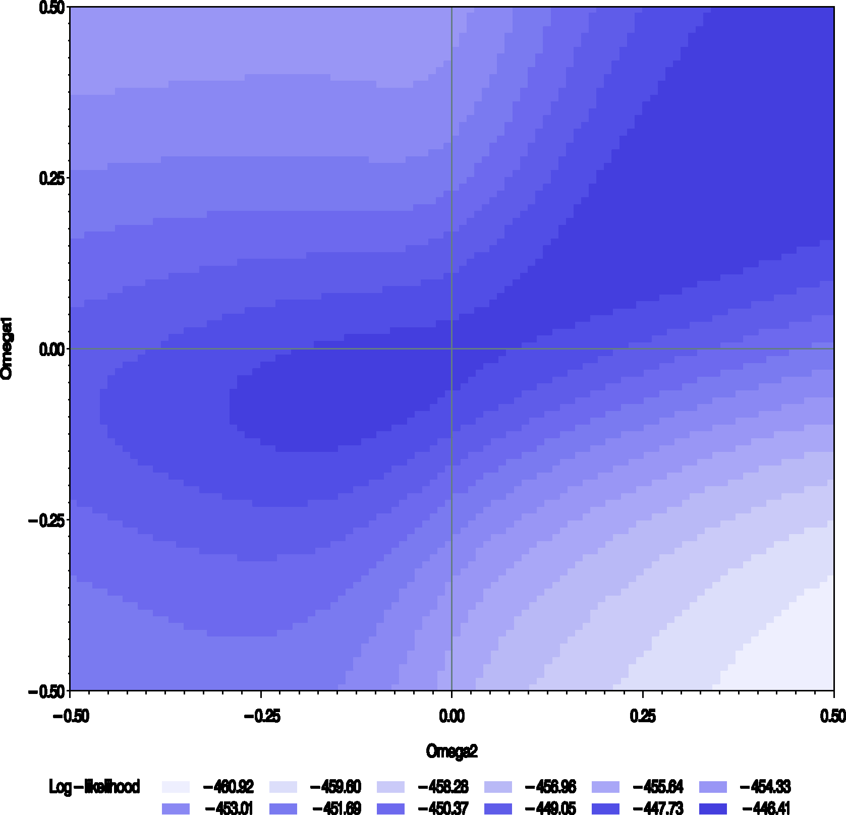
Contour plot of the profile log-likelihood from periods 1 and 3 of the Chow–Shao data set ( $- 0.5 \leq ω_{i} \leq 0.5$ ).

The profile likelihood has a maximum for values of ω around (0, 0) and along a stripe in the region where $ω_{1} ω_{2} > 0$ and decreases in the area $Ω_{-} = {ω_{1} ω_{2} < 0}$ . Hence, for both treatments it is more likely that MNAR works in the same direction. The parameter estimates corresponding to $Ω_{-}$ are $\leq 2$ or $\geq 7$ indicating that the MAR estimate is fairly robust against deviations from MAR under the multivariate normal model assumption.

5 Discussion

This paper has discussed aspects of the analysis of cross-over trials with incomplete data. In this context, we have argued that a mixed-effects model provides a valuable tool for the analyses of such trials. Consequently, recommendations and guidelines insisting on fixed-effect analyses may be unnecessarily rigid. When the model assumptions are appropriate, the mixed-model approach allows for a correct analysis under the MAR assumption by including all available measurements into the analysis, while the fixed-model analysis can only use within-subject information and provides a correct analysis only when MCAR holds.

Having said this it is fair to mention that one of the disadvantages of mixed-effects models is that the Wald statistics used to assess treatment effects are only approximately F-distributed and small sample corrections are required. The solution offered by Kenward and Roger¹⁷ is implemented in PROC MIXED of SAS¹⁸ and can be routinely used to relieve the issue.

In a well-designed cross-over trial without missing data, there is little information lost by discarding treatment information contained in the subject totals as done by using fixed-effects analyses. The introduction of random-subject effects into the model allows this information to be incorporated into the analysis when data are missing. In such an analysis, a weighted average is implicitly used that combines between- and within-subject effects. The weights are equal to the inverse of the variances of the two estimates (see Jones and Kenward,⁸ Chapter 5).

Although MAR does not constitute a reasonable assumption in all cases it is the most general assumption under which a valid analysis is possible without considering the missingness mechanism explicitly. Such an analysis can serve as a starting point for further investigations of the dependency of the results under different assumptions on the missingness mechanism. We provided such sensitivity analyses using the selection model factorization. The principles applied can be taken forward to more complex cross-over settings as well. It would be interesting to see how a sensitivity analysis would look like in the pattern mixture framework, though as seen in Section 2, the assumptions made for one have direct implications on the other.

Footnotes

Acknowledgement

The author is grateful to Michael G Kenward, London School of Hygiene and Tropical Medicine, for offering his comments and sharing his insights during the preparation of this paper and to an anonymous reviewer for his diligent and constructive review of the submitted manuscript.

Funding

This research received no specific grant from any funding agency in the public, commercial, or not-for-profit sectors.

Conflict of interest

None declared.

References

CHMP. Guideline on missing data in confirmatory clinical trials, European Medicines Agency, 2011.

Grizzle

. The two-period change-over design and its use in clinical trial. Biometrics 1965; 21: 467–480.

Patel

. Analysis of incomplete data in a two-period crossover design with reference to clinical trials. Biometrika 1985; 72: 41–418.

Kenward

Molenberghs

. Likelihood based frequentist inference when data are missing at random. Stat Sci 1998; 13: 236–247.

Lee

Kim

Park

. Average bioequivalence for two-sequence two period crossover design with incomplete data. J Biopharm Stat 2005; 15: 857–867.

Richardson

Flack

. The analysis of incomplete data in the three-period two-treatment cross-over design for clinical trials. Stat Med 1996; 15: 127–143.

Chow

Shao

. Statistical methods for two-sequence three-period cross-over designs with incomplete data. Stat Med 1997; 16: 103–1039.

Jones

Kenward

. Design and analysis of cross-over trials, 2nd ed. London: Chapman and Hall, 2003.

Basu

Santra

. A joint model for incomplete data in crossover trials. J Stat Plan Infer 2010; 140: 2839–2845.

10.

Diggle

Kenward

. Informative drop-out in longitudinal data analysis. Appl Stat 1994; 43: 457–472.

11.

CHMP. Guideline on the investigation of bioequivalence, European Medicines Agency, 2010.

12.

Guidance for industry: statistical approaches to establishing bioequivalence. Food and Drug Administration, 2001.

13.

Rubin

. Inference and missing data. Biometrika 1976; 63: 58–592.

14.

Kenward

. Selection models for repeated measurements with non-random dropout: an illustration of sensitivity. Stat Med 1998; 17: 2723–2732.

15.

Molenberghs

Verbeke

Thijs

. Influence analysis to assess sensitivity of the dropout process. Comput Stat Data Anal 2001; 37: 93–113.

16.

Kenward

Roger

. The use of baseline covariates in crossover studies. Biostatistics 2010; 11: 1–17.

17.

Kenward

Roger

. Small sample inference for fixed effects from restricted maximum likelihood. Biometrics 1997; 53: 983–997.

18.

SAS Institute Inc. SAS/STAT 9.22 user’s guide, Cary, NC: SAS Institute Inc., 2010.

19.

Molenberghs

Beunckens

Sotto

. Every missing not at random model has got a missing at random counterpart with equal fit. J R Stat Soc Ser B 2008; 70: 37–388.

20.

Liu

Pierce

. A note on Gauss-Hermite quadrature. Biometrika 1994; 81: 624–629.