Individual treatment effect prediction for amyotrophic lateral sclerosis patients

Abstract

A treatment for a complicated disease might be helpful for some but not all patients, which makes predicting the treatment effect for new patients important yet challenging. Here we develop a method for predicting the treatment effect based on patient characteristics and use it for predicting the effect of the only drug (Riluzole) approved for treating amyotrophic lateral sclerosis. Our proposed method of model-based random forests detects similarities in the treatment effect among patients and on this basis computes personalised models for new patients. The entire procedure focuses on a base model, which usually contains the treatment indicator as a single covariate and takes the survival time or a health or treatment success measurement as primary outcome. This base model is used both to grow the model-based trees within the forest, in which the patient characteristics that interact with the treatment are split variables, and to compute the personalised models, in which the similarity measurements enter as weights. We applied the personalised models using data from several clinical trials for amyotrophic lateral sclerosis from the Pooled Resource Open–Access Clinical Trials database. Our results indicate that some amyotrophic lateral sclerosis patients benefit more from the drug Riluzole than others. Our method allows gradually shifting from stratified medicine to personalised medicine and can also be used in assessing the treatment effect for other diseases studied in a clinical trial.

Keywords

Personalised medicine individual treatment effect random forest model-based recursive partitioning

1 Introduction

Amyotrophic lateral sclerosis (ALS) is a deadly disease that affects motor neurons in the brain and spinal cord, i.e. the neurons responsible for voluntary muscle control. Riluzole (Rilutek) is the only approved drug for this disease to date. According to the European Medicines Agency,¹ Riluzole prolongs the median survival of ALS patients, depending on the dose, by a few months. Several side effects, such as sickness, weakness or increased liver enzyme levels are mentioned.¹ Knowledge how Riluzole works on the nervous system of ALS patients is limited. The Pooled Resource Open–Access Clinical Trials (PRO-ACT) database² is the largest database containing clinical trial data of ALS patients available and was initiated to retrieve more information on the disease. It contains data from 17 ALS studies conducted between 1990 and 2010. Using these data, we aimed at finding out more about the effect of Riluzole on the health and survival of patients.

Before statistical analyses and p-values entered into medical progress 70 years ago, doctors treated patients individually based on their experiences and knowledge.³ Since the beginning of the ‘golden age of randomised clinical trials’, however, medication became more and more standardised. Nowadays, much knowledge about the effect of drugs has accumulated, cornerstone drugs such as antibiotics have been used for decades and many diseases can be treated successfully; however, providing new drugs for the general public becomes more difficult. Diseases such as ALS are too complex to treat all patients in the same way. Therefore, there is a need to return to more individualised treatments, but this time with the use of statistical concepts.

In the past years, there has been an immense effort towards personalised medicine in the analysis of randomised controlled trials. The goal is to identify predictive factors, i.e. factors that interact with the treatment,⁴ such as biomarkers, other treatments and environmental circumstances. In the following, we will refer to these factors as patient characteristics. Prognostic factors, i.e. factors that directly affect the patient’s outcome, are only of secondary interest, but should not be neglected, because they not only change the general level of the outcome – showing in the individual intercept – but might also be predictive and prognostic.⁵ Note that we use the terms predictive and prognostic as in the medical literature,⁴ but in a statistical sense both groups of variables are useful predictors. For drugs for which the biological mode of action is unknown, predictive and prognostic factors should first be identified in a data-driven way. New hypotheses can then be generated and new trials can be planned based on these hypotheses. In this first step, we ask whether a certain patient characteristic is relevant and not why.

Many new statistical methods in the field of stratified medicine, i.e. subgroup analysis, have been developed. Subgroup analyses aim at finding groups of patients that have differential treatment effects. Most of the methods are based on recursive partitioning (trees) and/or interaction models.^6–12 The tree-based methods for subgroup analyses have specialised splitting procedures for partitioning the patients into groups with higher and lower treatment effect. Interaction models evaluate the interaction between the treatment and given patient characteristics. The idea behind methods of subgroup analyses in general is to obtain a treatment effect $β (z)$ that depends on the patient characteristics z. For example, the treatment effect could depend on the age of patients, in which patients less than 40 years of age improve through the treatment, patients between 40 and 60 do not improve and patients older than 60 years improve, but less than the patients under 40 years:

β (z) = {\begin{matrix} 1 & if z_{age} < 40 \\ 0 & if 40 \leq z_{age} < 60 \\ 0.5 & if 60 \leq z_{age} \end{matrix}

(1)

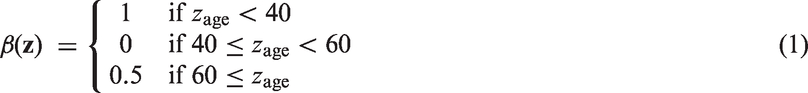
However, the assumption that the treatment effect is a step function may be too restrictive, and $β (z)$ in reality may be a smooth interaction function. In other words, personalised medicine is required instead of stratified medicine. Because methods for subgroup analyses again generalise the treatment effect for a group of patients, it can only be considered as a step in the direction toward personalised medicine. We provide a method that can estimate smooth treatment effect functions using model-based random forests and weighted models. More importantly, this method provides an estimate for the treatment effect of a future patient, thereby allowing a decision to be made whether treatment of this patient is appropriate.

2 Methods

Seibold et al., 2016⁵ introduced a means of conducting subgroup analysis for randomised controlled trials using model-based recursive partitioning. One first defines a model $M ((Y, X), ϑ)$ with primary endpoint Y, covariates X including the randomised treatment indicator

X_{A} = {\begin{matrix} 1 & if patient received the (new) treatment \\ 0 & if patient received no treatment (or standard of care), \end{matrix}

(2)

and parameter vector ϑ. In the following, we will consider likelihood models (e.g. generalised linear models or parametric survival models) where the model parameters ϑ can be estimated by maximising the log-likelihood

ℓ ((Y, X), ϑ)

of those models (e.g. Gaussian log-likelihood or Weibull log-likelihood) or equivalently by solving the score equation

\sum_{i = 1}^{N} s ((y, x)_{i}, ϑ) = 0

(3)

with

s ((y, x)_{i}, ϑ) = \frac{\partial ℓ ((y, x)_{i}, ϑ)}{\partial ϑ}

(4)

In most applications, the model contains only an intercept α and a treatment effect β, i.e. $X = (1, X_{A})$ and $ϑ = (α, β)^{⊤}$ , but more parameters are possible, such as coefficients of additional regressors or scale and shape parameters for the response distribution. Technically, there can also be more than two treatment groups or no intercept. For simplicity, we will focus on the basic case with intercept and treatment effect and two treatment groups. The method obtains subgroups ${B_{b = 1, \dots, B}}$ that differ with regard to the treatment effect β and potentially the intercept α. The subgroups are defined by patient characteristics $Z = (Z_{1}, \dots, Z_{J}) \in Z$ . Hence, the intercept and treatment parameters can be written as a function of the subgroup-defining variables z. In other words, the patient characteristics Z are not part of the model $M ((Y, X), ϑ)$ but are used to define the subgroups in which the model parameters differ, and then the model parameters are estimated within each subgroup.

Conceptually, the partitioned model parameters $α (z)$ and $β (z)$ might depend on z in a more complex way than a simple tree structure. Therefore, the model parameters are not step functions, but rather smooth interaction functions, so that an individual treatment effect (as in personalised medicine) can be computed for each patient instead of only for each subgroup of patients (as in stratified medicine). The function $β (z)$ can then be understood as an estimate of the counterfactual individual treatment effect of a patient with patient characteristics z.

The most intuitive step from a tree structure to a more complex structure is to use a random forest instead of a single tree. Hence, we propose a strategy in which a model-based random forest is used to measure how similar patients are with respect to the treatment effect and the treatment effect of each patient is predicted on this basis using personalised models.

2.1 Random forest

Random forests¹³ compute an ensemble of T trees. The proposed algorithm draws subsamples $L_{t}, t = 1, \dots, T$ of the given N observations and fits a model-based tree to each subsample using a randomly sampled set of candidate split variables z. The data $L_{t}^{c}$ that were not in the learning sample for tree t are called out-of-bag data. Classical random forests provide information on the similarity between observations with respect to the response. Model-based random forests provide information on the similarity between observations (patients) with respect to the model parameters, i.e. treatment effect and intercept.

This section focuses on the estimation of the trees, and the following section features the computation of the similarity measure and how the forest can be used to estimate personalised treatment effects.

2.2 Split procedure

The special feature of our method is the split procedure, which is based on the empirical estimating function

s = (\begin{matrix} s_{α} ((y, x)_{1}, \hat{ϑ}) & s_{β} ((y, x)_{1}, \hat{ϑ}) \\ s_{α} ((y, x)_{2}, \hat{ϑ}) & s_{β} ((y, x)_{2}, \hat{ϑ}) \\ : & : \\ s_{α} ((y, x)_{N}, \hat{ϑ}) & s_{β} ((y, x)_{N}, \hat{ϑ}) \end{matrix})

(5)

which contains the score contributions

s_{α} ((y, x)_{i}, \hat{ϑ})

and

s_{β} ((y, x)_{i}, \hat{ϑ})

. The score contributions are the partial derivatives of the log-likelihood with respect to α or β, respectively, evaluated at the N observed data points and the estimated parameters

\hat{ϑ} = (\hat{α}, \hat{β})^{⊤}

.¹⁴ The matrix of score contributions s contains information on the deviation from the model fit for all parameters and observations of a given model

M ((Y, X), ϑ)

. The contributions can thus be seen as residuals. Score contributions are widely used in model inference (e.g. see Chapter 3.7, Tutz, 2012)¹⁵ and in recursive partitioning.^14,16 They are particularly useful because they fluctuate randomly around 0 in well-fitting models, and they show patterns when there are parameter instabilities.

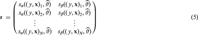
To obtain a split in model-based recursive partitioning for this setup, the following steps have to be performed:

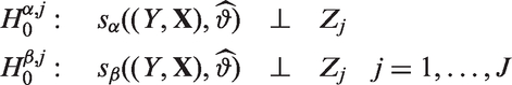
Estimate the parameters in the prespecified model $M ((Y, X), ϑ)$ .

Compute the associated score matrix s .

Perform tests of independence between the score contributions and the partitioning variables:

\begin{matrix} H_{0}^{α, j} : s_{α} ((Y, X), \hat{ϑ}) ⊥ Z_{j} \\ H_{0}^{β, j} : s_{β} ((Y, X), \hat{ϑ}) ⊥ Z_{j} j = 1, \dots, J \end{matrix}

The smallest p-value corresponds to the greatest deviation from the model assumption; that intercept and treatment parameter are the same for all patients in the given node/subgroup.

If any p-value is lower than the significance level, select the partitioning variable that has the highest association (lowest p-value) to any of the relevant residuals for the split.

Search for the optimal split point in the selected partitioning variable using a suitable criterion, such that the models in the resulting daughter nodes have as little association between the partitioning variable and the residuals as possible.

This split procedure is repeated until a stopping criterion is met. This can be, for example, when no p-values are lower than the significance level or if subgroups become too small. For detailed information on stopping criteria, see Hothorn et al., 2015.¹⁷ In the end, a tree is obtained with disjoint subgroups

⋃_{b}^{•} B_{b} = Z

(6)

Accordingly in a random forest of T trees, each tree defines disjoint subgroups

⋃_{b}^{•} B_{tb} = Z \forall t = 1, \dots, T

(7)

The independence tests can be performed using permutation tests^18,19 or, for reasonably large samples, using M-fluctuation tests.^14,20 Unbiased recursive partitioning methods commonly use tests with node-wise null hypotheses of ‘no further split needed’, as we do here.^14,16,19 Since one test is computed per patient characteristic eligible in the given node, multiplicity adjustment such as Bonferroni correction is recommended. More details on the algorithm and the test procedures used are documented in Appendix 2.

2.3 Personalised models

In personalised medicine, the goal is to learn how much a person will profit from a given treatment and what would happen if the standard of care or no treatment is given. For any patient, it is possible to compute a personalised model based on the similarity of this observation to the observations in the training data. In general, any measure of similarity $w_{i} (z_{k})$ between patients i and k with respect to the treatment effect and general health could be used, i.e. any measure that compares patients i and k in terms of $β (z_{i})$ to $β (z_{k})$ and of $α (z_{i})$ to $α (z_{k})$ . A straight forward similarity measure in this sense is the number of times patients i and k are classified in the same subgroup by the single model-based trees in the random forest

w_{i} (z_{k}) = \sum_{t = 1}^{T} \sum_{b = 1}^{B_{t}} (z_{i} \in B_{tb})^(z_{k} \in B_{tb})

(8)

with T being the number of trees used for the computation of the forest and B_t being the number of subgroups from tree t.^21–23 If patient i is part of the training set, the weights can be computed out-of-bag, i.e. the only trees (

t = 1, \dots, T

) considered are those where patient i is not in the subset

L_{t}

for the computation.

To obtain the personalised model $M ((Y, X), \hat{ϑ} (z_{i}))$ for patient i, the base model is recomputed with the weighted training data, which is equivalent to minimising the personal log-likelihood of patient i (the sum of weighted log-likelihood contributions)

\underset{ϑ}{arg max} \sum_{k = 1}^{N} w_{i} (z_{k}) \cdot ℓ ((y, x)_{k}, ϑ (z_{i}))

(9)

In other words, every patient k from the training set is included $w_{i} (z_{k})$ times in the ‘new data set’ to compute the personalised model for patient i. In the following, the parameters estimated from this model will be denoted by $\hat{ϑ} (z_{i}) = (\hat{α} (z_{i}), \hat{β} (z_{i}))$ .

Using the personalised models, it is possible to obtain a log-likelihood. From the personalised model for patient i, the log-likelihood contribution $ℓ ((y, x)_{i}, \hat{ϑ} (z_{i}))$ for this observation is computed. The log-likelihood then is

\sum_{i = 1}^{N} ℓ ((y, x)_{i}, \hat{ϑ} (z_{i}))

(10)

which we refer to as forest log-likelihood. A variant of this algorithm for non-personalised transformation models is discussed in Hothorn and Zeileis.²⁴

2.4 Improvement through personalised models

To check whether the personalised models actually lead to an improvement of the base model, one tests the hypothesis

\begin{matrix} H_{0} : \\ \underset{H_{0}^{α}}{\underset{︸}{α (Z) \equiv α}} \end{matrix}

(11)

\begin{matrix} \cap \\ \underset{H_{0}^{β}}{\underset{︸}{β (Z) \equiv β}} \end{matrix}

(12)

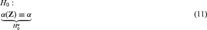
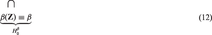
This strict null hypothesis is to be rejected if any of the patient characteristics contain information on the outcome or the treatment effect. To conduct the test, one can proceed as follows:

Compute the forest log-likelihood and the log-likelihood of the base model and calculate their difference. This difference is a measure of how much better the personalised models are compared to the base model.

Draw parametric bootstrap samples from the base model.

Compute the forest log-likelihood and the log-likelihood of the base model in the bootstrap samples and again compute the differences. The distribution of these values represents the distribution under the null hypothesis.

The p-value is then the proportion of bootstrap samples in which the difference in log-likelihoods exceeds the observed difference in the original data. Note, that this p-value will be very low or even 0 when the patient characteristics contain information on the outcome or the treatment effect.

In practice, one may be interested in just $H_{0}^{β}$ , but testing the sub-hypotheses $H_{0}^{α}$ and $H_{0}^{β}$ separately is not straight-forward. An approximation would be to compute the personalised models using a forest that splits based only on the partial score function with respect to α or β. Patient characteristics, however, are often not exclusively predictive or prognostic but can be both. Also, if a patient characteristic is purely prognostic, this still may result in a pattern in both partial score functions. For more details, see Seibold et al, 2016.⁵

2.5 Dependence plots

A partial dependence plot describes the dependence of a function (in our case the treatment effect $\hat{β} (z)$ ) and a variable (in our case, a partitioning variable).²⁵ The partial dependence plot resulting from a model-based tree would show a step function. The partial dependence from a random forest can be smoother for continuous partitioning variables. It can be obtained by plotting $\hat{β} (z_{j})$ against z_j for each partitioning variable $j = 1, \dots, J$ .

2.6 Variable importance

The variable importance for the random forest is computed based on the tree log-likelihoods. For a given forest computed with T trees, the log-likelihood is computed as follows:

Select the out-of-bag data $L_{t}^{c}$ and determine the terminal node/subgroup to which each observation i belongs.

Compute the log-likelihood contribution of each observation $i \in L_{t}^{c}$ based on the respective model in the terminal node/subgroup with parameters $\hat{ϑ} (z_{i})$ .

Compute the out-of-bag log-likelihood as the sum of the contributions

ℓ_{t} = \sum_{i \in L_{t}^{c}} ℓ ((y, x)_{i}, \hat{ϑ} (z_{i}))

(13)

To obtain the variable importance of a given variable

z_{j}, j = 1, \dots, J

, the variable is permuted. The log-likelihood is computed as above, except that the column with information about z_j in the out-of-bag data is replaced by the permuted z_j. We denote the log-likelihood of tree t with variable z_j permuted by

ℓ_{t}^{(j)}

. The variable importance is then

{VI}_{j} = \frac{1}{T} \sum_{t = 1}^{T} [ℓ_{t} - ℓ_{t}^{(j)}]

(14)

If the variable importance is high, the variable is an important predictive and/or prognostic factor. Note that due to the signed differences, the variable importances might become negative signalling that the log-likelihood merely improved by chance and that the variable is not important. As the size of the negative values conveys information on the overall importance variability, we do not collapse to 0 which would otherwise be a sensible restriction. It is possible to compute also conditional variable importances²⁶ to account for correlation between patient characteristics. In the following, we focus on unconditional variable importances.

3 Results

3.1 PRO-ACT data

The PRO-ACT (https://nctu.partners.org/ProACT) database contains longitudinal data of ALS patients that participated in one of 16 phase II and III trials and one observational study. It is a project initiated by the non-profit organisation Prize4Life (http://www.prize4life.org/) to enhance knowledge about ALS. It contains information on a broad variety of patient characteristics, such as vital signs, the patient’s and family’s history, and treatment information. Identification criteria, such as study centres, are not included in the database. Also collected are the survival time and the ALS functional rating scale (ALSFRS), which is a score measuring the patients’ ability of living a normal life.²⁷ The ALSFRS is a sum-score of 10 items, each of which ranges between 0 and 4, where 0 represents complete inability and 4 represents normal ability. The items are speech, salivation, swallowing, hand-writing, cutting food and handling utensils, dressing and hygiene, turning in bed and adjusting bed clothes, walking, climbing stairs and breathing. As outcomes in the study, we used both the survival time (denoted by survival) and the ALSFRS 6 months after treatment start (denoted by ${ALSFRS}_{6}$ ) and identified patient characteristics that influence the effect of Riluzole on these outcomes. For the two outcome variables, we obtained two different data sets. We only included observations that contain information on the respective outcome variable and only patient characteristics that have fewer than 50% missing values. The survival time data set contains 3306 observations and 18 patient characteristics. The ALSFRS data set contains 2534 observations and 57 patient characteristics.

Tables 1 and 2 show the estimates including standard errors obtained from the base model for each outcome. For the ALSFRS, this base model is given by

E (\frac{{ALSFRS}_{6}}{{ALSFRS}_{0}} | X = x) = \frac{E ({ALSFRS}_{6} | X = x)}{{ALSFRS}_{0}} = exp {α + β x_{A}}

(15)

which represents a Gaussian generalised linear model with log-link and offset

log ({ALSFRS}_{0})

, where

{ALSFRS}_{0}

is the ALSFRS that was measured at the time of treatment start. The base model for the survival time is given by the Weibull model

ℙ (T \leq survival | X = x) = F (\frac{log (survival) - α_{1} - β x_{A}}{α_{2}})

(16)

where F is the cumulative distribution function of the Gompertz distribution. Note that the Weibull model has a scale parameter in addition to the intercept, so that both α₁ and α₂ control the appearance of the baseline hazard. In the notation of equation (4), this leads to

ϑ = (α_{1}, α_{2}, β)^{⊤}

Table 1.

ALSFRS base model (Gaussian generalised linear model with log-link and offset).

	Estimate	Std. error	2.5%	97.5%
α	−0.1595	0.0065	−0.1722	−0.1468
β	0.0091	0.0077	−0.0060	0.0242

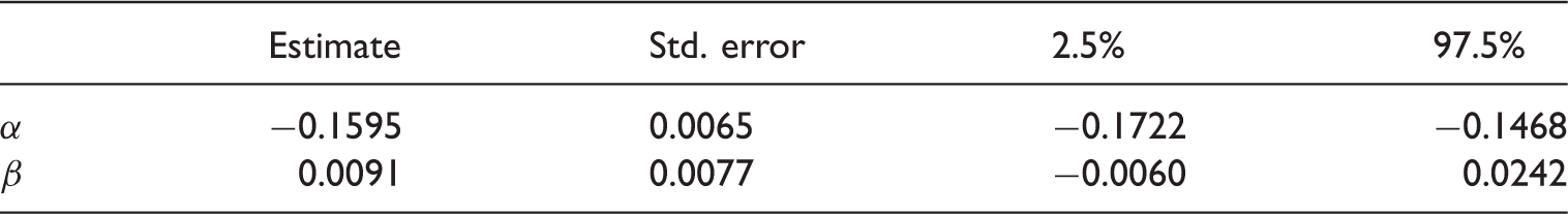
Given are the parameter estimates, their standard error and the Wald confidence interval.

Table 2.

Survival time base model (Weibull model).

	Estimate	Std. error	2.5%	97.5%
α ₁	6.7070	0.0323	6.6437	6.7703
β	0.1073	0.0387	0.0314	0.1832
$log (α_{2})$	−0.5833	0.0271	−0.6364	−0.5302

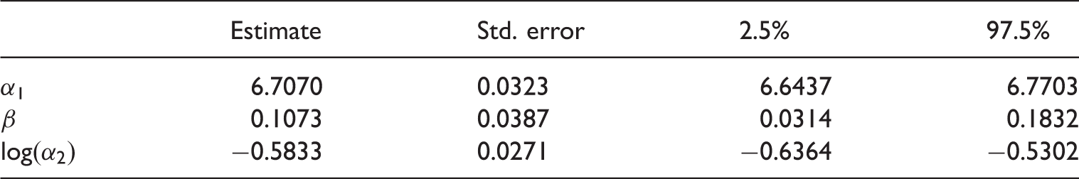
Given are the parameter estimates, their standard error and the Wald confidence interval.

3.2 Personalised models

We computed personalised models for all observations in the respective training data, which were used to obtain the random forest. The distribution of parameter estimates in the personalised models is given in Figure 1 for the ALSFRS and in Figure 2 for the survival time. Figure 1 shows that all patients are predicted to have a positive Riluzole effect, i.e. for all patients taking Riluzole, a higher ALSFRS is achieved compared to those not taking Riluzole. However, there is a variability in the treatment effects, and the distribution of the treatment effect is bimodal (as is the distribution of the intercept). The treatment effect estimated from the base model is between the two modes. The lowest treatment effect a person in this data set is predicted to have is 0.0027.

Figure 1.

Kernel density estimates of the personalised parameter estimates for the ALSFRS.

Figure 2.

Distribution of the personalised parameter estimates for the survival time. The baseline hazard functions are given in the left panel; the kernel density estimate of the treatment effect estimate is given in the right panel.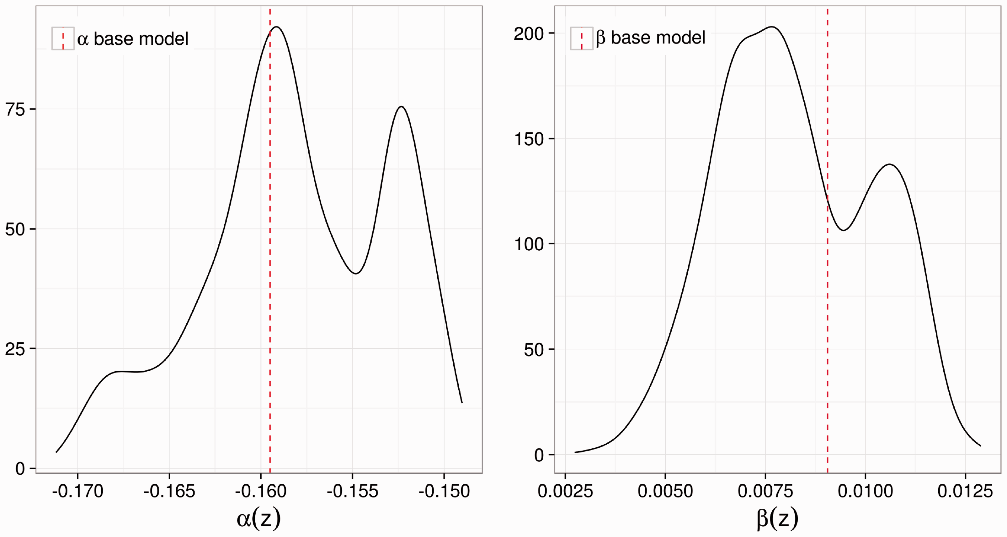

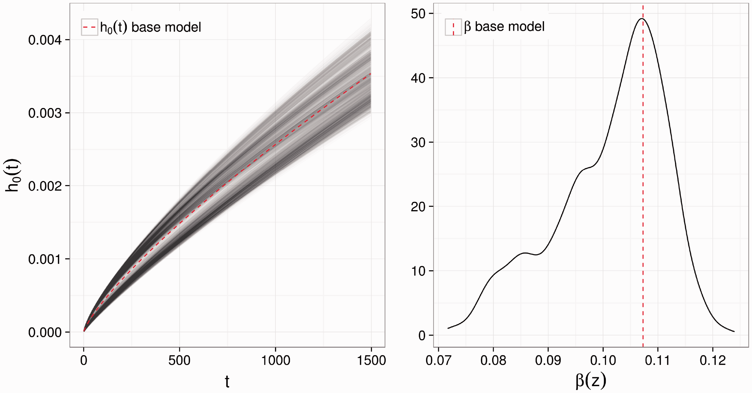
For the survival time, the lowest predicted treatment effect is 0.0717. However, the value of the treatment effect in the personalised survival models cannot be interpreted in isolation; its meaning depends on the shape of the baseline hazard, i.e. on α₁ and α₂. Instead of depicting the densities of the two baseline hazard parameters, in Figure 2, we show the baseline hazard curves. The baseline hazard varies for different patients, and there is a gap in the middle. The baseline hazard estimated from the base model lies close to that gap.

From the personalised models, we obtained the ‘forest log-likelihoods’ for both outcomes. For the Gaussian GLM with log-link and offset, the log-likelihood contribution for observation i is defined as

\begin{matrix} l (({ALSFRS}_{6}, {ALSFRS}_{0}, x)_{i}, \hat{ϑ} (z_{i})) \\ = ({ALSFRS}_{6 i} - exp (x_{i}^{⊤} \hat{ϑ} (z_{i})) \cdot {ALSFRS}_{0 i})^{2} \end{matrix}

(17)

with

x_{i} = (1, x_{Ai})^{⊤}

and

\hat{ϑ} (z_{i}) = (\hat{α} (z_{i}), \hat{β} (z_{i}))^{⊤}

. For the Weibull model, the log-likelihood contribution for observation i is

\begin{matrix} l ((survival, x)_{i}, \hat{ϑ} (z_{i})) = δ_{i} log ({\hat{α}}_{2} (z_{i})) - δ_{i} \frac{{survival}_{i} - x_{i}^{⊤} {\hat{ϑ}}^{*} (z_{i})}{{\hat{α}}_{2} (z_{i})} + exp (\frac{{survival}_{i} - x_{i}^{⊤} {\hat{ϑ}}^{*} (z_{i})}{{\hat{α}}_{2} (z_{i})}) \end{matrix}

(18)

with

x_{i} = (1, x_{iA})^{⊤}

{\hat{ϑ}}^{*} (z_{i}) = ({\hat{α}}_{1} (z_{i}), \hat{β} (z_{i}))^{⊤}

and δ_i as the censoring indicator.

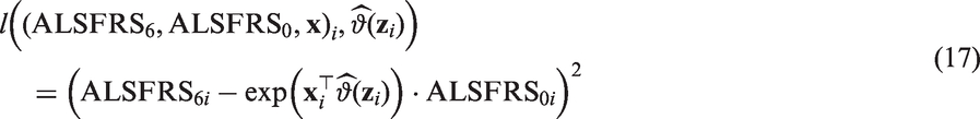
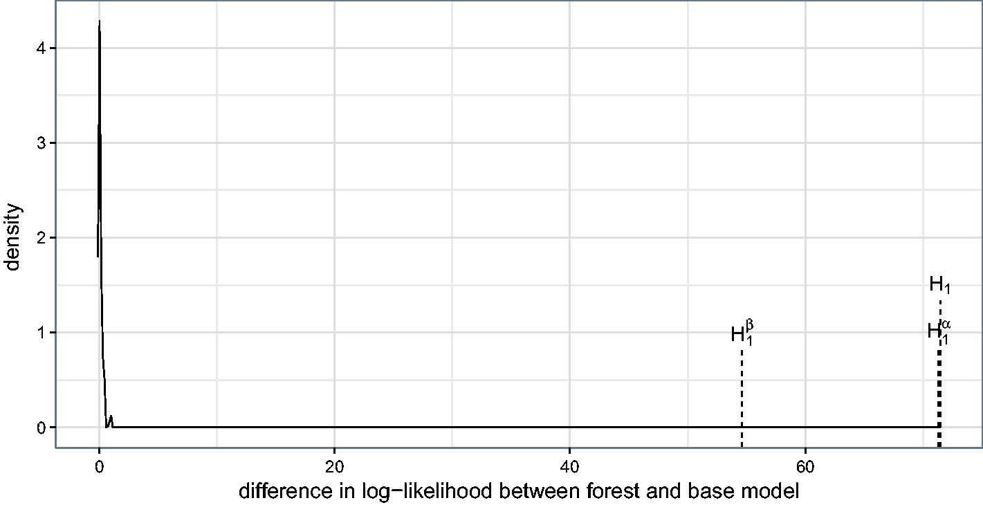
As can be seen in Figures 3 and 4, the forest log-likelihoods are higher than the log-likelihoods of the base models for both the ALSFRS and the survival time. The figures show the difference in log-likelihood between the forest and the corresponding base model. To show that this difference is not due to overfitting, we drew 50 samples from the base models, i.e. 50 parametric bootstrap samples for which the assumption holds that the intercept (or baseline hazard) and treatment effect are the same for all patients. ALSFRS values are drawn from a normal distribution truncated at 0 to assure positivity. (The effect of truncation is virtually negligible; only two observations had a truncation probability of more than 1%.) The survival times are drawn from a Weibull distribution censored at the originally observed censoring times (if exceeded). The differences in log-likelihoods for both ALSFRS and survival time are distributed close to 0, with a slight shift to the right, for the parametric bootstrap samples. The large difference in the ALS data supports the assumption that the base models are not ideal and personalised models are meaningful (the respective p-values are both 0). To approximately check the sub-hypotheses given in equations (11) and (12), we also computed log-likelihoods of the two forests that split only with respect to one of the partial score functions – either intercept (or baseline hazard) or treatment effect. For the ALSFRS, both the forest under 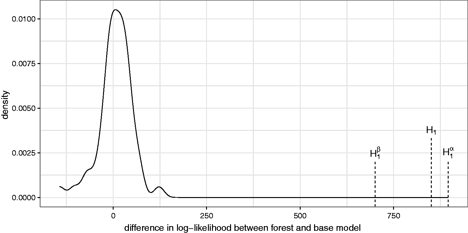$H_{1}^{α}$ (computed with splitting only based on the partial score function with respect to the intercept α) and the forest under $H_{1}^{β}$ (computed with splitting only based on partial score function with respect to the treatment effect β) lead to greatly improved models compared to the base model. The difference in log-likelihood between the forest under $H_{1}^{α}$ and the base model is even greater than between the original forest (H₁) and the base model. For the survival time, the log-likelihoods of the original forest and the forest under $H_{1}^{α}$ (based on splits in the partial score function with respect to the baseline hazard) are very close to each other. Splitting based only on the partial score function with respect to the treatment effect ( $H_{1}^{β}$ ) already improves the log-likelihood but not as much as splitting based on both intercept and treatment effect (H₁). The good performances of the forests under $H_{1}^{α}$ indicate that (a) there are no predictive patient characteristics, (b) all predictive patient characteristics are also prognostic or (c) the predictive nature of the predictive patient characteristics are so strong that it has enough impact on the structure of the partial score function with respect to α.

Figure 3.

Difference in log-likelihoods between forest and base model using the original data (dashed lines; H₁, the usual forest; $H_{1}^{α}$ , the forest that splits based on α; $H_{1}^{β}$ , the forest that splits based on β) and using 50 samples simulated from the base model (density curve) for the ALSFRS outcome.

Figure 4.

3.3 Dependence plots

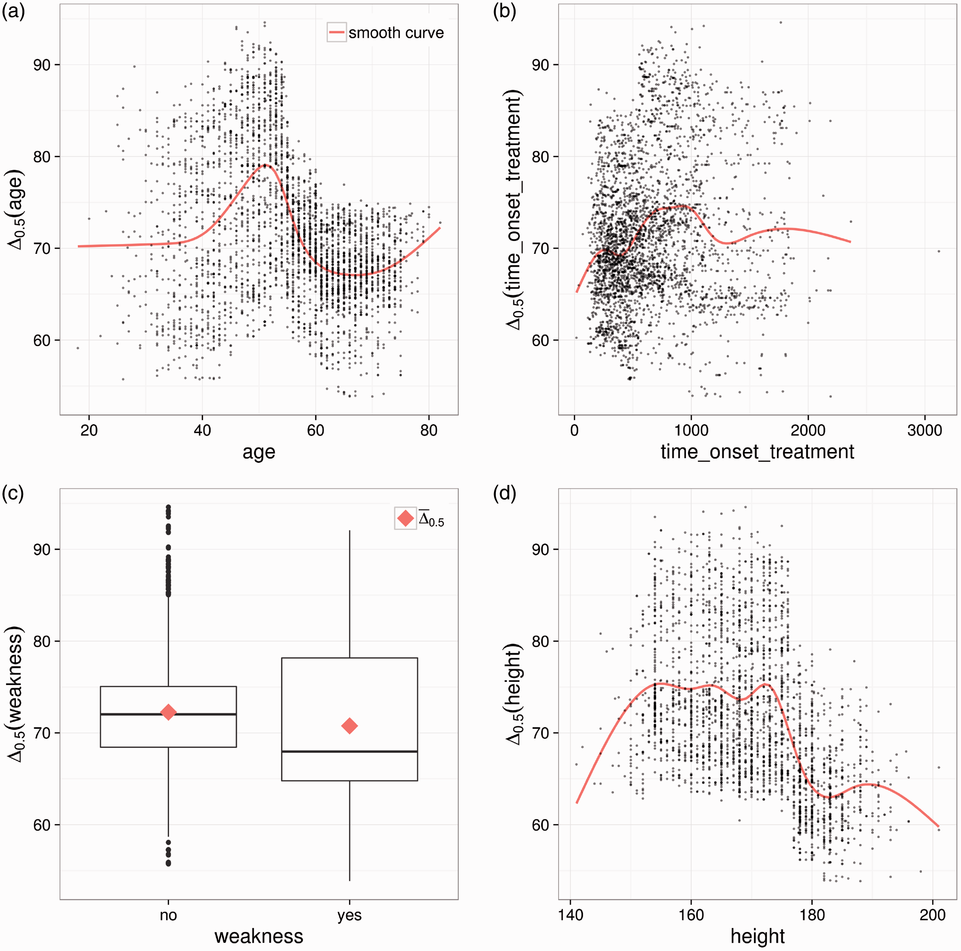
The dependence plots as shown in Figures 5 and 6 can be obtained for any partitioning variable. Here we show the dependence plots for the four variables with the highest variable importance (see Section 3.4). For continuous variables, such as age, we show a scatter plot, as before. For categorical variables, such as the variable weakness, which indicates whether a patient suffers from muscle weakness (yes/no), boxplots giving the variation of $β (z)$ and a square representing $\bar{β} (z)$ , i.e. the mean, are a meaningful way of representing the dependence between treatment effect and the given variable.

Figure 5.

Dependence plots for the four patient characteristics with the highest variable importance from the ALSFRS forest. (a) Dependence plot for the time in days between disease onset and treatment start. (b) Dependence plot for the creatinine level in mmol/L. (c) Dependence plot for the phosphorus level in mmol/L. (d) Dependence plot for the forced vital capacity (volume of air in litres that can forcibly be blown out after full inspiration).

Figure 6.

Dependence plots for the four patient characteristics with the highest variable importance from the survival time forest. (a) Dependence plot for the age. (b) Dependence plot for the time in days between disease onset and treatment start. Outlier has been omitted in the estimation of the smooth curve. (c) Dependence plot for the weakness indicator. (d) Dependence plot for the height.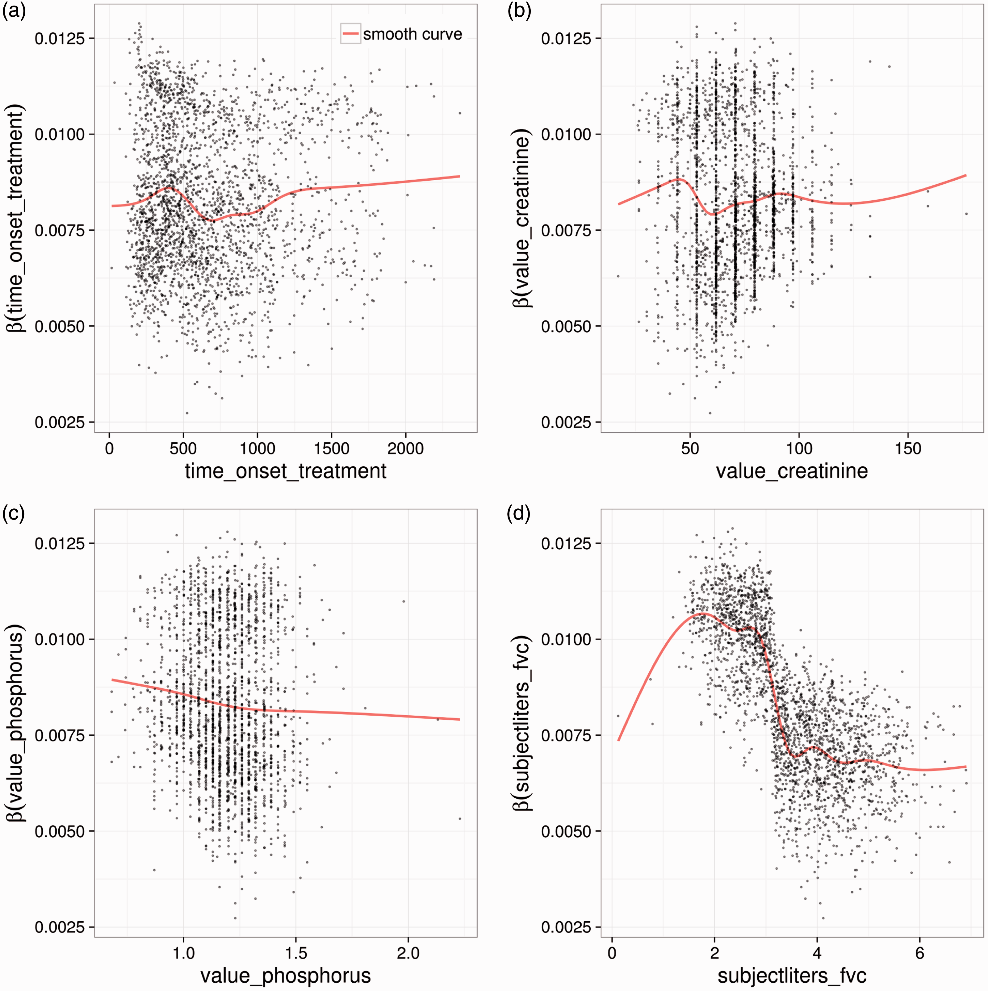

The most obvious pattern of the four graphs in Figure 5 is shown in Figure 5(d), in which the personalised treatment effects are plotted against the forced vital capacity (FVC). Patients with a low lung function (low FVC) are predicted to have a higher treatment effect than those with better lung function. The graph shows a relatively clear cut at approximately 3 L. This indicates that FVC is a predictive factor. For the time between disease onset and treatment start, the pattern is less clear. Patients with a short as well as those with a long time between disease onset and treatment start seem to benefit most. Also for the creatinine value, which indicates kidney function, only weak patterns are observed. The phosphorus balance is slightly negatively associated with the treatment effect.

For the survival time, plotting only the treatment effect against a variable is not meaningful since the interpretation of the treatment effect depends on the shape of the baseline hazard. Therefore, we took a different approach in this case and show on the y-axis the difference in median survival between treatment and control intake. For example, a value of 70 means that based on the personalised model of this patient, the median survival is prolonged by 70 days if the patient takes Riluzole. The difference in median survival is denoted by $Δ_{0.5}$ . Any other quantile could be used as well since from the Weibull model, information on the entire estimated distribution in the two treatment groups is obtained. Taking the difference in medians makes sense because it is a measure on the scale of the outcome, just as the treatment effect in a linear model, which is the difference in means. The shape of $Δ_{0.5}$ when plotted against age shows a strong pattern that indicates that age is a predictive factor (see Figure 6). The treatment efficacy increases with age until about 55 years and then flattens. The difference in median survival slightly increases with the days between disease onset and start of treatment in the beginning, but decreases again after about 1000 days. Patients who suffer from weakness have a greater variance in their benefit from Riluzole. Tall patients are predicted to benefit little on average.

3.4 Variable importance

Figures 7 and 8 show the variable importance of each split variable. Figure 7 suggests that the time between disease onset and start of treatment plays the most important role for the personalised models. The time between disease onset and start of treatment, the FVC, and the phosphorus balance have been shown to be the most important variables for stratified models,⁵ which is underlined by this analysis. The time between disease onset and start of treatment contains information on the state of disease progression for patients in the trial. If the disease onset and the start of treatment are far apart, the patient is likely to have a slow progression.²⁸ Also Riluzole has been shown to not be effective when the disease is already far progressed.¹ Thus, it is not surprising that this variable is selected as an important variable.

Figure 7.

Variable importances of all split variables used for the ALSFRS forest.

Figure 8.

Variable importances of all split variables used for the survival time forest.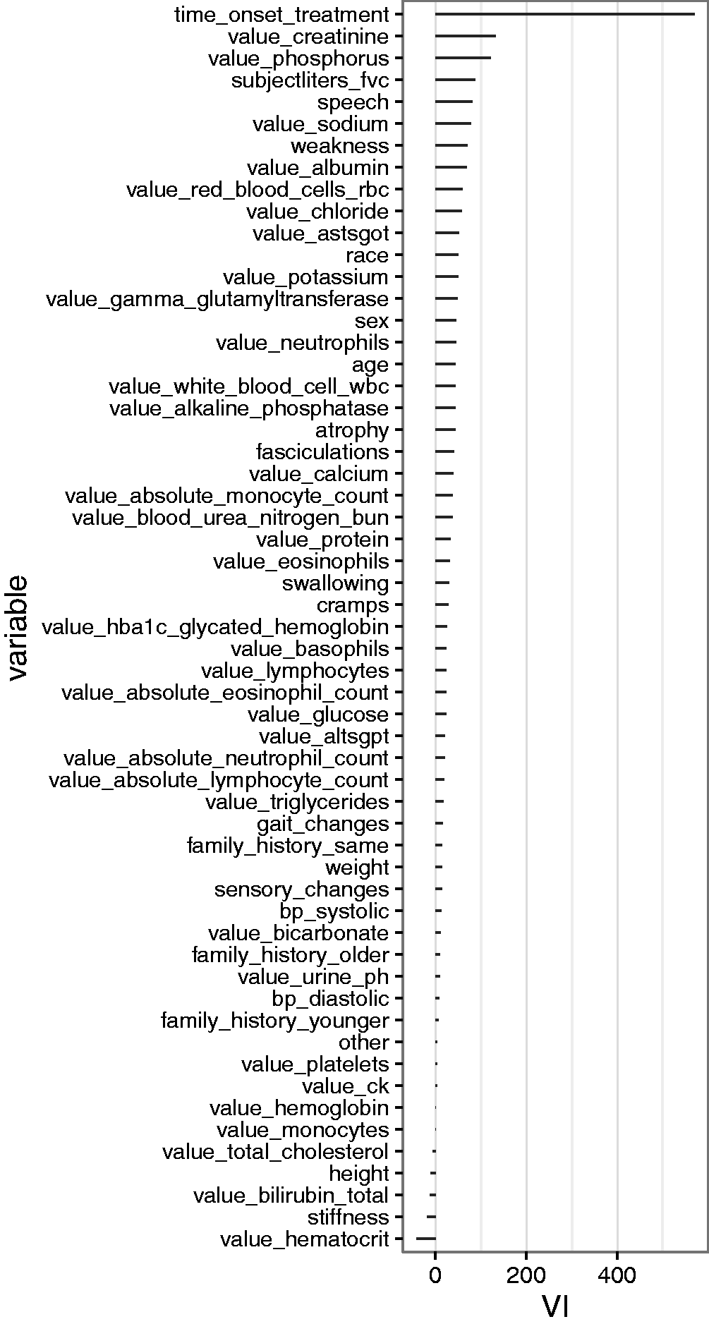

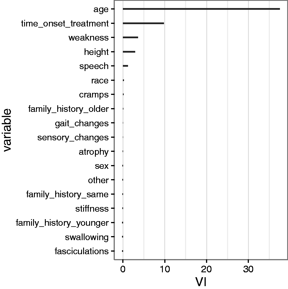
For the Riluzole effect on the survival time, the patient’s age and again the time between onset and treatment start play a role. Both variables have been identified before⁵ as important factors for survival time.

4 Discussion

Model-based forests can find important predictive and prognostic patient characteristics and – more importantly – via the personalised models provide the possibility to predict the counterfactual individual treatment effect of a future patient. The personalised models allow a shift from standardised medicine back to personalised medicine, but this time in a controlled way by using statistical principles. Through analysis of the PRO-ACT data and simulations (see Appendix 3), we showed that personalised models can perform better than the standard global model if there are differences in treatment effect between patients. If there is no difference, the performance of the methods is about the same. In our performance checks, we focused on the fit of the model to the data based on the log-likelihood. Performance of the method for new patients was studied using simulations.

The proposed method is applicable to clinical trial data where treatment is randomised. In our analysis of the PRO-ACT data, we included several clinical trials for which we have no knowledge about inclusion criteria or any other details of the study protocol as this information is not given out in order to anonymise data. This could possibly lead to confounding issues. As there is interest in methodology for when treatment is not randomised, we included a small simulation study on this topic in Appendix 4. The results seem promising in the case where the patient characteristic that impacts the treatment assignment is not the predictive factor. However, there is a bias when a patient characteristic is predictive and also impacts treatment assignment. Further work in the area of observational trials is needed where, e.g. adjustment methods such as propensity scoring²⁹ could be of use.

The presented methods are based on tree-based subgroup analyses but go a step further. Not only are subgroups identified and the treatment effect within each group estimated, but many slightly varying trees are used to retrieve a measure of similarity between patients. On this basis, a model is computed in which more similar patients are weighted higher. The personalised models provide point estimates for the treatment effect. When the individual treatment effects are plotted against patient characteristics, researchers can determine whether the patient characteristics are predictive factors and in what way the patient characteristics and the treatment interact. For ALS patients, the FVC value was predictive for the ALSFRS, and the patient’s age and height were predictive for survival. The next step would be to generate hypotheses from these findings and plan a study to test these. Our method offers a promising means of providing individual treatment effect predictions and can be applied to any clinical trial data where baseline patient characteristics are available.

All results were obtained solely using open-source implementation software (see Section 5), which provides easy access to the methods.

5 Computational details

The code for data preprocessing of the PRO-ACT data is available in the TH.data package.³⁰ The source code for the full analyses is available on https://github.com/HeidiSeibold/personalised_medicine. Implementation of all methods discussed in this article is based on the R partykit package (version 1.0-2).³¹ Other R packages used were sandwich (2.3-3),^32,33 survival (2.38-1),³⁴ eha (2.4-2)³⁵ and ggplot2 (2.0.0).³⁶ All computations were conducted in the R system for statistical computing (version 3.2.0).³⁷

Footnotes

Acknowledgements

We thank Karen A. Brune for improving the language.

Declaration of conflicting interests

The author(s) declared no potential conflicts of interest with respect to the research, authorship, and/or publication of this article.

Funding

The author(s) disclosed receipt of the following financial support for the research, authorship, and/or publication of this article: Heidi Seibold and Torsten Hothorn were financially supported by the Swiss National Science Foundation (Grant 205321_163456).

References

European Medicines Agency. Riluzole Zentiva: EPAR summary for the public, http://www.ema.europa.eu/docs/en_GB/document_library/EPAR_-_Summary_for_the_public/human/002622/WC500127609.pdf (2012, accessed 28 January 2017).

Atassi

Berry

Shui

et al.

The PRO-ACT database: Design, initial analyses, and predictive features. Neurology 2014; 83: 1719–1725.

Weisberg

. What next for randomised clinical trials? Significance 2015; 12: 22–27.

Italiano

. Prognostic or predictive? It’s time to get back to definitions!. J Clin Oncol 2011; 29: 4718–4718.

Seibold

Zeileis

Hothorn

. Model-based recursive partitioning for subgroup analyses. Int J Biostat 2016; 12: 45–63.

Ciampi

Negassa

Lou

. Tree-structured prediction for censored survival-data and the Cox model. J Clin Epidemiol 1995; 48: 675–689.

Kehl

Ulm

. Responder identification in clinical trials with censored data. Comput Stat Data Anal 2006; 50: 1338–1355.

Dusseldorp

Van Mechelen

. Qualitative interaction trees: A tool to identify qualitative treatment-subgroup interactions. Stat Med 2013; 33: 219–237.

Loh

Man

. A regression tree approach to identifying subgroups with differential treatment effects. Stat Med 2015; 34: 1818–1833.

10.

Tian

Alizadeh

Gentles

et al.

A simple method for estimating interactions between a treatment and a large number of covariates. J Am Stat Assoc 2014; 109: 1517–1532.

11.

Foster

Taylor

JMG

Kaciroti

et al.

Simple subgroup approximations to optimal treatment regimes from randomized clinical trial data. Biostatistics 2015; 16: 368–382.

12.

Zhang

Tsiatis

Davidian

et al.

Estimating optimal treatment regimes from a classification perspective. Stat 2012; 1: 103–114.

13.

Breiman

. Random forests. Mach Learn 2001; 45: 5–32.

14.

Zeileis

Hothorn

Hornik

. Model-based recursive partitioning. J Comput Graph Stat 2008; 17: 492–514.

15.

Tutz

. Regression for categorical data, New York: Cambridge University Press, 2012.

16.

Loh

. Regression trees with unbiased variable selection and interaction detection. Stat Sin 2002; 12: 361–386.

17.

Hothorn T, Hornik K and Zeileis A. ctree: Conditional inference trees, Vignette R package partykit version 1.1-1, https://CRAN.R-project.org/web/packages/partykit/vignettes/ctree.pdf (2016, accessed 28 January 2017).

18.

Hothorn

Hornik

Van de Wiel

et al.

A Lego system for conditional inference. Am Stat 2006; 60: 257–263.

19.

Hothorn

Hornik

Zeileis

. Unbiased recursive partitioning: A conditional inference framework. J Comput Graph Stat 2006; 15: 651–674.

20.

Zeileis

Hornik

. Generalized M-fluctuation tests for parameter instability. Stat Neerland 2007; 61: 488–508.

21.

Hothorn

Lausen

Benner

et al.

Bagging survival trees. Stat Med 2004; 23: 77–91.

22.

Meinshausen

. Quantile regression forests. J Mach Learn Res 2006; 7: 983–999.

23.

Lin

Jeon

. Random forests and adaptive nearest neighbors. J Am Stat Assoc 2006; 101: 578–590.

24.

Hothorn T and Zeileis A. Transformation forests. Technical Report, arXiv 1701.02110, v1, https://arxiv.org/abs/1701.02110 (2017, accessed 28 January 2017).

25.

Hastie

Tibshirani

Friedman

. The elements of statistical learning. 2nd ed, Berlin: Springer-Verlag, 2009.

26.

Strobl

Boulesteix

Kneib

et al.

Conditional variable importance for random forests. BMC Bioinform 2008; 9: 307–307.

27.

Brooks

Sanjak

Ringel

et al.

The amyotrophic lateral sclerosis functional rating scale – assessment of activities of daily living in patients with amyotrophic lateral sclerosis. Archiv Neurol 1996; 53: 141–147.

28.

Hothorn

Jung

. RandomForest4life: A random forest for predicting ALS disease progression. Amyotrop Lateral Scler Frontotemp Degen 2014; 15: 444–452.

29.

Rosenbaum

Rubin

. The central role of the propensity score in observational studies for causal effects. Biometrika 1983; 70: 41–55.

30.

Hothorn T. TH.data: TH’s data archive, R package version 1.0-7, https://CRAN.R-project.org/package=TH.data (2016, accessed 28 January 2017).

31.

Hothorn

Zeileis

. partykit: A modular toolkit for recursive partytioning in R. J Mach Learn Res 2015; 16: 3905–3909.

32.

Zeileis

. Econometric computing with HC and HAC covariance matrix estimators. J Stat Softw 2004; 11: 1–17.

33.

Zeileis

. Object-oriented computation of sandwich estimators. J Stat Softw 2006; 16: 1–16.

34.

Therneau TM. A package for survival analysis in S, Version 2.40-1, https://CRAN.R-project.org/package=survival (2016, accessed 28 January 2017).

35.

Broström G. eha: Event history analysis, R package version 2.4-4, https://CRAN.R-project.org/package=eha (2016, accessed 28 January 2017).

36.

Wickham

. ggplot2: Elegant graphics for data analysis, New York: Springer-Verlag, 2009.

37.

R Core Team. R: A language and environment for statistical computing, Vienna, Austria: R Foundation for Statistical Computing, 2016.

38.

Strasser

Weber

. On the asymptotic theory of permutation statistics. Mathem Method Stat 1999; 8: 220–250.

39.

Strobl

Boulesteix

Zeileis

et al.

Bias in random forest variable importance measures: Illustrations, sources and a solution. BMC Bioinform 2007; 8: 25–25.

40.

Foster

Taylor

Ruberg

. Subgroup identification from randomized clinical trial data. Stat Med 2011; 30: 2867–2880.