Extended negative binomial hurdle models

Abstract

Poisson models are widely used for statistical inference on count data. However, zero-inflation or zero-deflation with either overdispersion or underdispersion could occur. Currently, there is no available model for count data, that allows excessive occurrence of zeros along with underdispersion in non-zero counts, even though there have been reported necessity of such models. Furthermore, given an excessive zero rate, we need a model that allows a larger degree of overdispersion than existing models. In this paper, we use a random-effect model to produce a general statistical model for accommodating such phenomenon occurring in real data analyses.

Keywords

Excessive zeros hierarchical generalized linear model Poisson hurdle model underdispersion zero-inflated Poisson model

1 Introduction

Poisson models provide a standard framework for analysis of count data. However, the requirement of equality of the mean and variance is sometimes restrictive. For example, we often encounter overdispersed data where the sample variance is greater than the sample mean. A negative binomial (NB) model¹ can be used for the analysis of such overdispersed count data. Underdispersion, where the variance is less than the mean, occurs less frequently and the choice of distributions is much narrower. However, there are situations in which underdispersion is well documented, such as in the study of polyspermy^2,3 and superparasitism.^4,5 Furthermore, the count data often have a higher incidence of zero counts than that is expected from the model. For excessive zeros, the zero-inflated Poisson (ZIP),⁶ the zero-inflated NB (ZINB),⁷ Poisson hurdle (PH)⁸ and NB hurdle (NBH)⁹ models have been proposed. Even though these models are often found suitable for analyzing excessive zero counts, they do not allow excessive zeros in addition to underdispersion in non-zero counts. However, such phenomenon occurs in practice. Lee et al.¹⁰ illustrated that high spatial correlation among counts can cause severe excessive zeros, so that an underdispersed quasi-Poisson hierarchical generalized linear model (HGLM)¹¹ would be useful for the analysis of spatial data. Chernyavskiy et al.¹² showed that such model is recommended for the analysis of cohort data. In this paper, we introduce extended NBH (ENBH) models to accommodate various phenomena encountered in data analysis.

In section 2, we present motivarint examples to illustrate the need for the ENBH model. In section 3, we review existing models and in section 4 we investigate properties of ENBH models. In section 5, we show the performance of the proposed model via simulation studies. All proofs are in the Supplementary material.

2 Examples

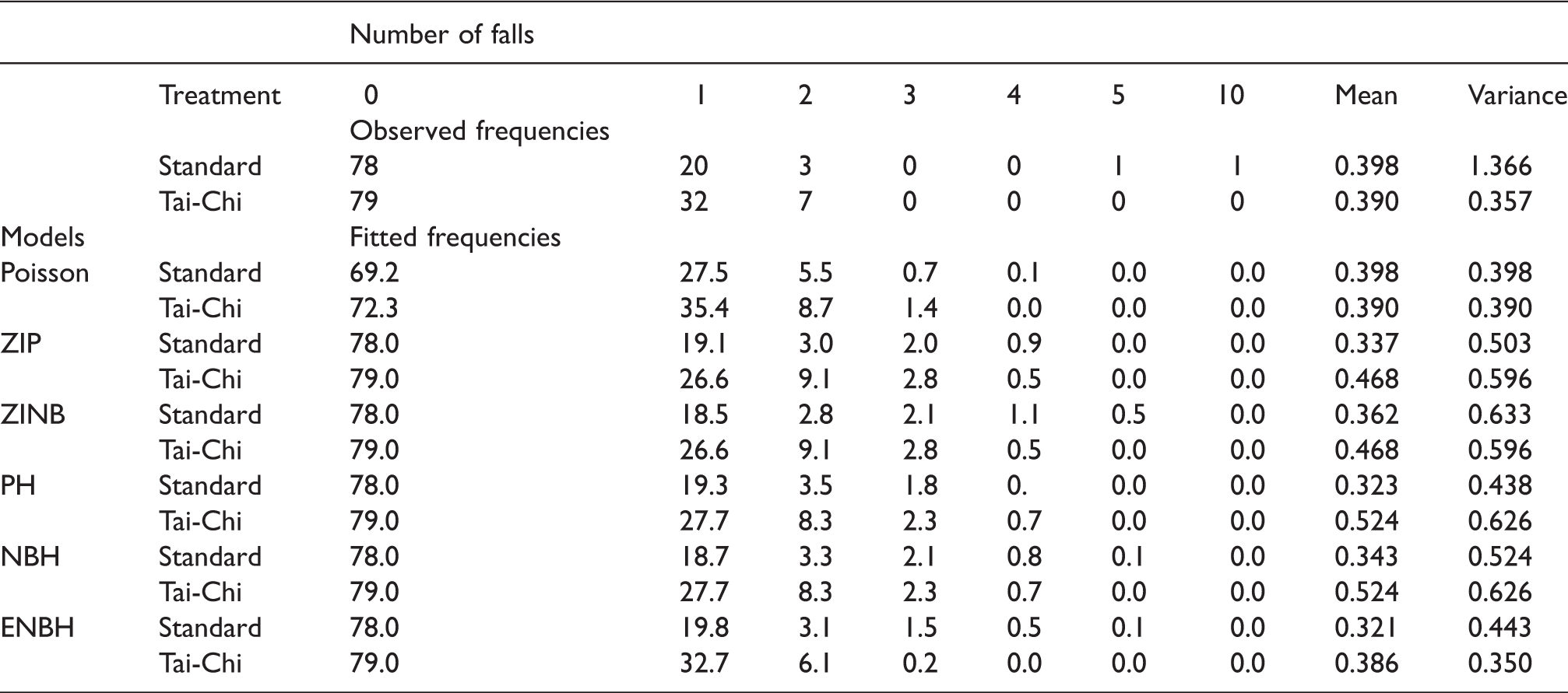
Molas and Lesaffre¹³ introduced a data set from an intervention study on the number of falls in elderly people. Falls are a common problem among the elderly. Between 55 and 70 percent of fall incidents result in physical injury. The effect of Tai-Chi Chuan exercises is examined on reducing the frequency of falls in healthy elderly people living at home who are at an increased risk of falling. Table 1 presents the frequency of falls in the two treatments for the fourth period in Molas and Lesaffre.¹³ Data from the group with Tai-Chi exercises show excessive number of zero counts with underdispersion. From the table we see that existing models such as the ZIP, ZINB, PH, and NBH models explain excessive zeros better than the Poisson data. However, these models allow only overdispersion when excessive zeros occur. Given the excessive zero rate, the ENBH model produces the best fitting frequencies of the data. For the group with standard exercises, if we delete the two outlying patients with 5 and 10 falls, the underdispersion among non-zero counts is evident.

Table 1.

Frequency table for the fourth visit in Molas and Lesaffre (2010) data set.

		Number of falls
	Treatment	0	1	2	3	4	5	10	Mean	Variance
		Observed frequencies
	Standard	78	20	3	0	0	1	1	0.398	1.366
	Tai-Chi	79	32	7	0	0	0	0	0.390	0.357
Models		Fitted frequencies
Poisson	Standard	69.2	27.5	5.5	0.7	0.1	0.0	0.0	0.398	0.398
	Tai-Chi	72.3	35.4	8.7	1.4	0.0	0.0	0.0	0.390	0.390
ZIP	Standard	78.0	19.1	3.0	2.0	0.9	0.0	0.0	0.337	0.503
	Tai-Chi	79.0	26.6	9.1	2.8	0.5	0.0	0.0	0.468	0.596
ZINB	Standard	78.0	18.5	2.8	2.1	1.1	0.5	0.0	0.362	0.633
	Tai-Chi	79.0	26.6	9.1	2.8	0.5	0.0	0.0	0.468	0.596
PH	Standard	78.0	19.3	3.5	1.8	0.	0.0	0.0	0.323	0.438
	Tai-Chi	79.0	27.7	8.3	2.3	0.7	0.0	0.0	0.524	0.626
NBH	Standard	78.0	18.7	3.3	2.1	0.8	0.1	0.0	0.343	0.524
	Tai-Chi	79.0	27.7	8.3	2.3	0.7	0.0	0.0	0.524	0.626
ENBH	Standard	78.0	19.8	3.1	1.5	0.5	0.1	0.0	0.321	0.443
	Tai-Chi	79.0	32.7	6.1	0.2	0.0	0.0	0.0	0.386	0.350

Note: Fitted frequencies are from Poisson, ZIP, ZINB, PH, NBH and ENBH models.

Now using various data sets, we illustrate the usefulness of the ENBH model for data analysis. To evaluate the performance of prediction accuracy of the model, the whole data set is divided randomly into 70% as the training set and 30% as the test set repeatedly for 100 times. The predicted mean square error (PMSE) is computed for the test set by using the formula

PMSE = \frac{1}{n_{test}} \sum_{i = 1}^{n_{test}} (y_{i} - \hat{E (Y_{i})})^{2}

where n_test is the sample size of the test set, y_i is the response of the test set and

\hat{E (Y_{i})}

is the estimator of

E (Y_{i})

using the training data set. The model with a smaller PMSE is expected to have a better prediction of future observations. For a choice of model, we use the PMSE and the AIC (Akaike information criteria). For nested models, likelihood ratio is useful for a choice of model, while for non-nested models the AIC is useful.

2.1 Analysis of hospitalization

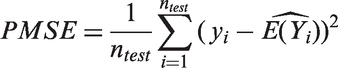
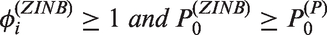
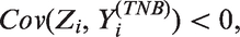
More than 71 million individuals in the United States are admitted to a hospital each year, according to a survey from the American Hospital Association.¹⁴ Studies concluded in 2006 that well over $30 billion was spent on unnecessary hospital admissions. So, it is very important to have a model for accurate prediction of hospitalization. The National Health and Nutrition Examination Survey of 2003–2004 has a total of 10,117 cases with hospitalization information. Around 90% of the cases have no incidence of hospitalization in the 12-month survey period. In Figure 1, the sample variances are below the sample means for most age groups. Tin¹⁴ noted that an underdispersion of hospitalization but with an excessive number of zero counts occurs in the data. However, there was no existing statistical model to account for this phenomenon.

Figure 1.

Means and variances for number of hospitalization by age group.

Now, consider the ENBH model with age as the only covariate

log (μ_{i}^{(ENBH)}) = β_{10} + β_{11} x_{i} and log {p_{i}^{Z} / (1 - p_{i}^{Z})} = β_{20} + β_{21} x_{i}

where

p_{i}^{Z}

is the probability of non-zero counts. Table 2 shows parameter estimates from the Poisson, ZIP, ZINB, PH, NBH and ENBH models. The parameter estimates for ξ in ZINB and NBH models are very close to 0. Thus, the ZINB and NBH models give identical results to those of the ZIP and PH models, respectively.

Table 2.

Hospitalization data: parameter estimates (standard errors) from the Poisson, ZIP, ZINB, PH, NBH and ENBH models.

	Poisson	ZIP, ZINB	PH, NBH	ENBH
Model for $E (Y_{i})$
Intercept	–2.61 (0.069)	–0.47 (0.082)	–0.60 (0.082)	–0.14 (0.031)
Age/10	0.19 (0.013)	0.070 (0.014)	0.066 (0.014)	0.025 (0.012)
Model for $p_{i}^{Z}$
Intercept		–1.19 (0.057)	–2.01 (0.092)	–0.81 (0.050)
Age/10		0.14 (0.018)	0.14 (0.017)	–0.02 (0.021)
$\hat{δ}$				–3.79 (0.84)
$\hat{ξ}$		0.00	0.00	0.54 (0.13)
$- 2 \sum log L (θ; y_{i})$	9250.7	8583.1, 8583.1	8026.5, 8026.5	7999.6
AIC	9254.7	8591.1, 8593.1	8034.5, 8036.5	8020.7
PMSE	0.217	0.209	0.206	0.192

PMSE: predicted mean square error; ZIP: zero-inflated Poisson; ZINB: zero-inflated NB; PH: Poisson hurdle; NBH: NB hurdle; ENBH: extended NBH.

For model choice, AIC and PMSE clearly indicate that the ENBH is the best among models considered. As we shall show, the ENBH model with δ = 0 is the NBH model. For testing δ = 0, the likelihood-ratio test (LRT) for NBH and ENBH 26.9(=8026.5–7999.6) >3.84 is significant at a level 0.05. Thus, the ENBH model should be selected.

In the ENBH, $\hat{δ} = - 3.79$ , implying that this data-set requires an underdispersion model with excessive zeros as discussed in Section 4.1. The effect of age is positively significant for $p_{i}^{Z}$ in the ZIP and PH models. With the ENBH model with negative $\hat{δ}$ , the age effect is no longer significant for $p_{i}^{Z}$ .

2.2 Analysis of reindeer pellet-group counts

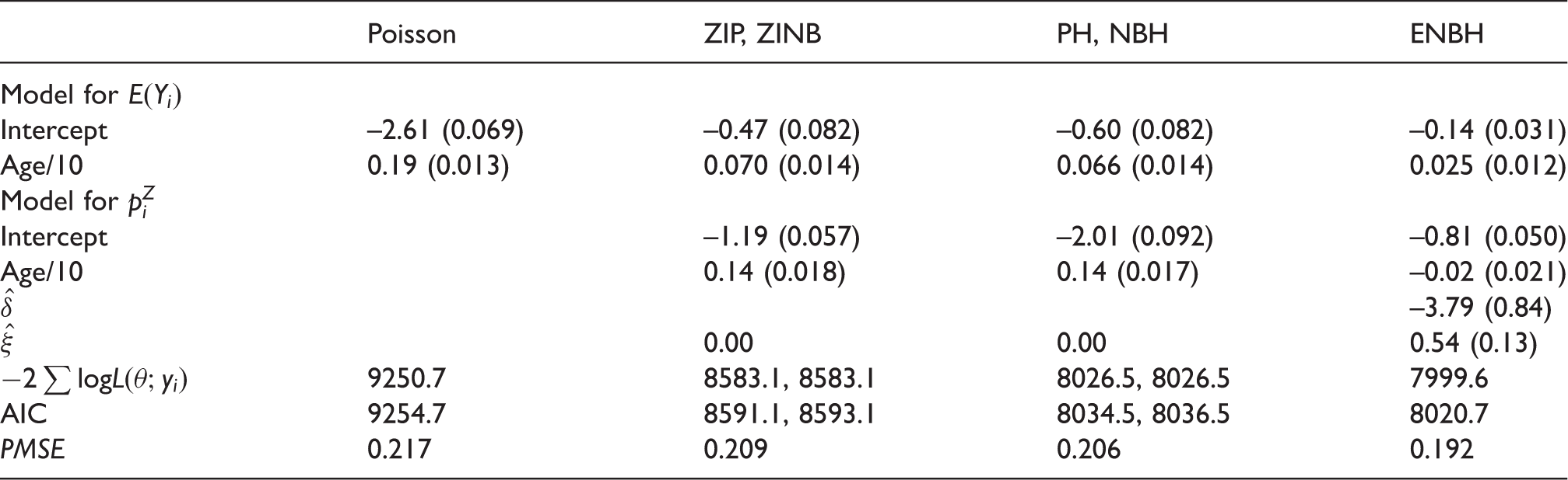
Lee et al.¹⁰ analyzed a data set on reindeer fecal pellet-group counts. For illustration, we use 2010 data. A pellet group was counted if the center of the group was found inside the plot. As an animal might move as it defecates, the pellets could spread over a large area. Therefore, a pellet group was defined by a cluster of 20 or more pellets. In order to model preference of reindeer grazing area, we model the pellet-group count. Lee et al.¹⁰ noted that 83.62% had zero counts in 2010. They showed that the ZIP, ZINB and PH models were not appropriate to fit this data-set since this data-set reveals underdispersion with excessive zeros. They used the quasi-Poisson-HGLM with spatial correlation as a final model which allows underdispersion. However, we prefer a real statistical model because a quasi-model poses difficulty in estimating parameters efficiently.¹⁵

In this paper, we consider a ENBH model using covariates of Lee et al.¹⁰

log (μ_{i}^{(ENBH)}) = X_{i}^{T} β_{1} + v_{i} and log {p_{i}^{Z} / ({1 - p}_{i}^{Z})} {= X}_{i}^{T} β_{2}

where

v = (v_{1}, \dots, v_{n})^{T} \sim N (0, Σ)

. For spatial covariance matrix Σ, we consider a Markov random field model in Lee et al.¹⁰ For model of

p_{i}^{Z}

, all covariates are not significant. Thus, we fit the intercept only model. Table 3 shows results of parameter estimates from quasi-Poisson-HGLM and ENBH models with the same spatial correlation structure. The quasi-Poisson-HGLM fit shows underdispersion

\hat{φ} = 0.48,

which corresponds to a negative

\hat{δ} = - 2.13

in the ENBH model. We see that AIC and PMSE criteria select the ENBH model. Quasi-Poisson-HGLM and ENBH are not nested, so that we may have a model choice based on the AIC. The AIC choose the ENBH since it is better than quasi-Poisson-HGLM. The PMSE shows that it has a better prediction.

Table 3.

Reindeer pellet-group counts data: parameter estimates (standard errors) from quasi-Poisson-HGLM and ENBH.

	quasi-Poisson-HGLM	ENBH
Model for $E (Y_{i})$
Intercept	–10.98 (5.16)	–9.54 (5.29)
Southeast slope	0.99 (0.41)	1.14 (0.42)
Elevation	–0.005 (0.004)	–0.005 (0.004)
Distance to power lines	1.33 (0.60)	1.27 (0.62)
Model for $p_{i}^{Z}$
Intercept		–2.13 (0.37)
$\hat{τ}$	2.33 (0.39)	2.14 (0.36)
$\hat{φ}$	0.48 (0.036)
$\hat{ξ}$		1.68 (0.53)
$\hat{δ}$		–2.13 (0.36)
$\hat{ρ}$	1.90 (0.42)	1.75 (0.44)
$- 2 \sum log L (θ; y_{i})$	−328.6	−337.7
AIC	−314.6	−319.7
PMSE	0.115	0.098

PMSE: predicted mean square error; ENBH: extended NBH; HGLM: hierarchical generalized linear model.

2.3 Demand for medical care by the elderly

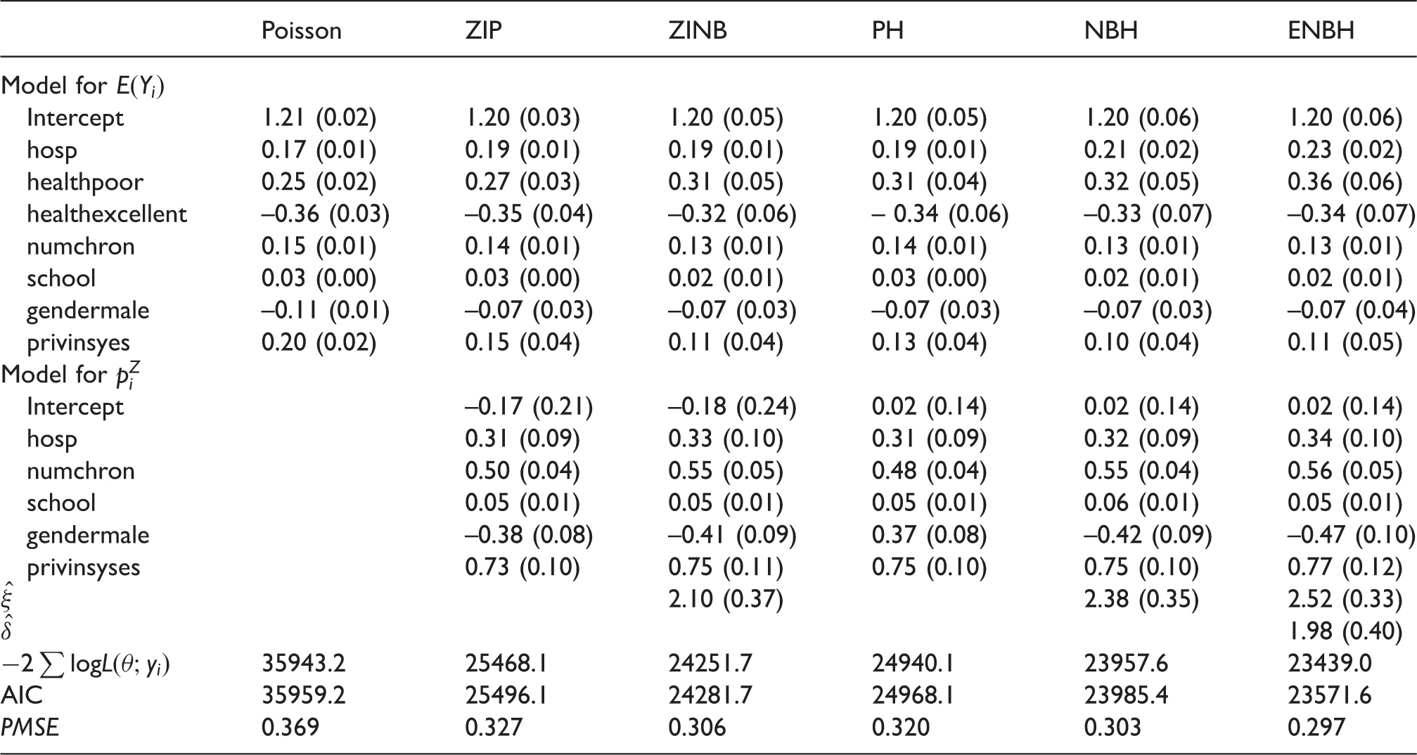
Deb and Trivedi¹⁶ analyzed data on 4406 individuals, aged 66 and over, who are covered by Medicare (a public insurance program), originally obtained from the US National Medical Expenditure Survey for 1987–1988. The objective is to model the demand for medical care as captured by the number of physician/non-physician office and hospital outpatient visits by the covariates available for the patients. Here, we adopt the number of physician office visits as the dependent variable and use the health status variables of hosp (number of hospital stays), health (self-perceived health status), numchron (number of chronic conditions), as well as the socioeconomic variables of gender, school (number of years of education), and privinsyes (private insurance indicator) as covariates.

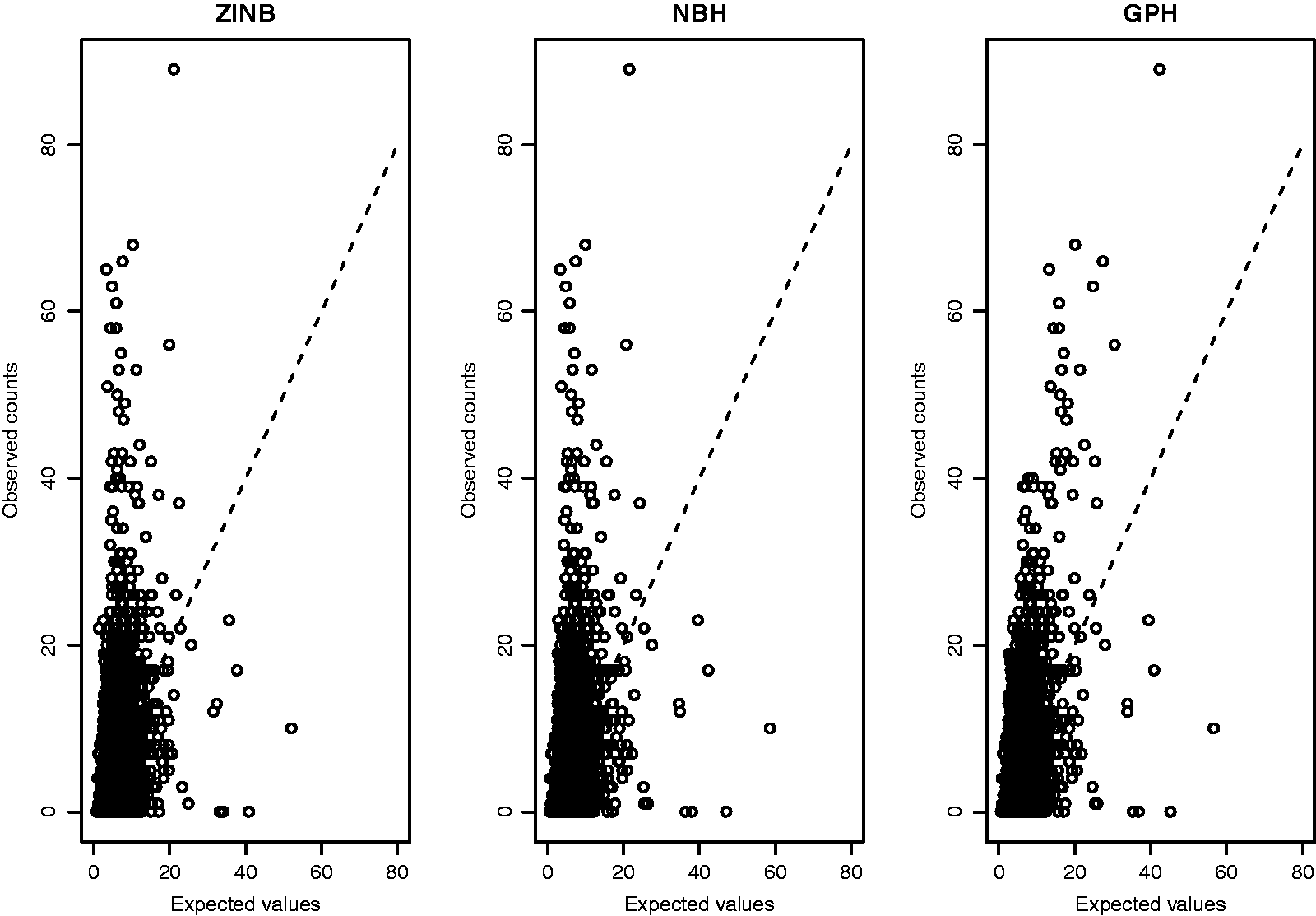
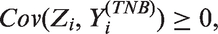
Table 4 shows results of parameter estimates from the Poisson, ZIP, ZINB, PH, NBH and ENBH models. In ENBH, we have $\hat{δ} = 1.98$ and $\hat{ξ} = 2.52$ , which implies that this data set has overdispersion with zero-inflation. Thus, all the models, ZIP, ZINB, PH, NBH and ENBH, could be potentially useful. Among them, AIC and PMSE select ENBH as the best. For testing δ = 0, the LRT for NBH and ENBH 518.6(=23957.6–23439.0) >3.84 is significant at a level 0.05. Thus, the ENBH model is selected. Because $\hat{δ} > 0$ , we have ${\hat{φ}}_{i}^{(ENBH)} \geq {\hat{φ}}_{i}^{(NBH)} \geq {\hat{φ}}_{i}^{(PH)} \geq 1$ . Thus, given zero-inflation, the ENBH model allows the largest overdispersion. Figure 2 plots the observed responses against the fitted values from the three models (ZINB, NBH and ENBH), which shows large overdispersion and excessive zeros. Figure 2 shows that the ENBH gives the best prediction model.

Figure 2.

Plots of expected values vs. observed counts for the ZINB, NBH and ENBH models.

Table 4.

Parameter estimates (standard errors) from Poisson, ZIP, ZINB, PH, NBH, and ENBH models for National Medical Expenditure Survey data.

	Poisson	ZIP	ZINB	PH	NBH	ENBH
Model for $E (Y_{i})$
Intercept	1.21 (0.02)	1.20 (0.03)	1.20 (0.05)	1.20 (0.05)	1.20 (0.06)	1.20 (0.06)
hosp	0.17 (0.01)	0.19 (0.01)	0.19 (0.01)	0.19 (0.01)	0.21 (0.02)	0.23 (0.02)
healthpoor	0.25 (0.02)	0.27 (0.03)	0.31 (0.05)	0.31 (0.04)	0.32 (0.05)	0.36 (0.06)
healthexcellent	–0.36 (0.03)	–0.35 (0.04)	–0.32 (0.06)	– 0.34 (0.06)	–0.33 (0.07)	–0.34 (0.07)
numchron	0.15 (0.01)	0.14 (0.01)	0.13 (0.01)	0.14 (0.01)	0.13 (0.01)	0.13 (0.01)
school	0.03 (0.00)	0.03 (0.00)	0.02 (0.01)	0.03 (0.00)	0.02 (0.01)	0.02 (0.01)
gendermale	–0.11 (0.01)	–0.07 (0.03)	–0.07 (0.03)	–0.07 (0.03)	–0.07 (0.03)	–0.07 (0.04)
privinsyes	0.20 (0.02)	0.15 (0.04)	0.11 (0.04)	0.13 (0.04)	0.10 (0.04)	0.11 (0.05)
Model for $p_{i}^{Z}$
Intercept		–0.17 (0.21)	–0.18 (0.24)	0.02 (0.14)	0.02 (0.14)	0.02 (0.14)
hosp		0.31 (0.09)	0.33 (0.10)	0.31 (0.09)	0.32 (0.09)	0.34 (0.10)
numchron		0.50 (0.04)	0.55 (0.05)	0.48 (0.04)	0.55 (0.04)	0.56 (0.05)
school		0.05 (0.01)	0.05 (0.01)	0.05 (0.01)	0.06 (0.01)	0.05 (0.01)
gendermale		–0.38 (0.08)	–0.41 (0.09)	0.37 (0.08)	–0.42 (0.09)	–0.47 (0.10)
privinsyses		0.73 (0.10)	0.75 (0.11)	0.75 (0.10)	0.75 (0.10)	0.77 (0.12)
$\hat{ξ}$			2.10 (0.37)		2.38 (0.35)	2.52 (0.33)
$\hat{δ}$						1.98 (0.40)
$- 2 \sum log L (θ; y_{i})$	35943.2	25468.1	24251.7	24940.1	23957.6	23439.0
AIC	35959.2	25496.1	24281.7	24968.1	23985.4	23571.6
PMSE	0.369	0.327	0.306	0.320	0.303	0.297

ZIP: zero-inflated Poisson; ZINB: zero-inflated NB; PH: Poisson hurdle; NBH: NB hurdle; ENBH: extended NBH.

We use the PMSE as a cross-validation of the proposed model. Throughout all three examples, the ENBH model has the smallest PMSE, so that it has the best predictions of future observations.

3 Class of models for excessive number of zero counts

In this paper, we consider a class of models for count response data $Y_{i}^{(M)}$ , having

μ_{i}^{(M)} = E (Y_{i}^{(M)}), var (Y_{i}^{(M)}) = φ_{i}^{(M)} μ_{i}^{(M)} and P_{0}^{(M)} = P (Y_{i}^{(M)} = 0)

Let $Y_{i}^{(P)}$ be the Poisson random variable with the mean

μ_{i}^{(P)} = E (Y_{i}^{(P)})

In the Poisson model, we have

E (Y_{i}^{(P)}) = var (Y_{i}^{(P)}) = μ_{i}^{(P)}, φ_{i}^{(P)} = 1 and P_{0}^{(P)} = P (Y_{i}^{(P)} = 0) = exp (- μ_{i}^{(P)})

The mean equals the variance and the probability of zero counts decreases as the mean increases. However, we often encounter count data, which exhibit overdispersion and an excessive number of zeros.

Conditioning on random effect u_i, suppose that $Y_{i}^{(NB)} | u_{i}$ follows the Poisson distribution with conditional mean

E (Y_{i}^{(NB)} | u_{i}) = μ_{i}^{(P)} u_{i}

where u_i follows the gamma distribution satisfying

E (u_{i}) = 1

and

var (u_{i}) = ξ

.¹⁵ Then,

Y_{i}^{(NB)}

follows marginally the negative-binomial (NB) distribution. The heterogeneity among u_i increases with ξ. In the NB model, we have

μ_{i}^{(NB)} = μ_{i}^{(P)} and φ_{i}^{(NB)} = 1 + ξ μ_{i}^{(NB)} \geq 1

Thus, in the NB model the extra-Poisson variation

ξ μ_{i}^{(NB)}

is caused by heterogeneity among

u_{i} .

Since

P_{0}^{(NB)} = (1 + ξ μ_{i}^{(NB)})^{- 1 / ξ} \geq P_{0}^{(P)}

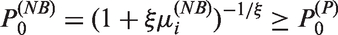
where the equality holds iff ξ = 0, the NB model with ξ > 0 always exhibits an overdispersion with excessive zeros. However, in practice, the probability of zero counts could be higher than the NB model for a given mean value. The mean, variance and zero probability of each model are in Table 5. Detailed derivations are in the supplementary materials.

Table 5.

Summary of mean, variance and zero probability for each of models.

Model	μ_i	φ_i	P ₀
Poisson	$μ_{i}^{(P)}$	1	$P_{0}^{(P)} = exp (- μ_{i}^{(P)})$
NB	$μ_{i}^{(P)}$	$1 + ξ μ_{i}^{(P)}$	$P_{0}^{(NB)} = 1 / (1 + ξ μ_{i}^{(P)})^{1 / ξ}$
ZIP	$p_{i}^{Z} μ_{i}^{(P)}$	$1 + (1 - p_{i}^{Z}) μ_{i}^{(P)}$	$1 - p_{i}^{Z} + p_{i}^{Z} P_{0}^{(P)}$
ZINB	$p_{i}^{Z} μ_{i}^{(P)}$	$1 + (1 - p_{i}^{Z}) μ_{i}^{(P)} + ξ μ_{i}^{(P)}$	$1 - p_{i}^{Z} + p_{i}^{Z} P_{0}^{(NB)}$
PH	$p_{i}^{Z} μ_{i}^{(P)} / {1 - P_{0}^{(P)}}$	$1 + μ_{i}^{(P)} {1 - p_{i}^{Z} - P_{0}^{(P)}} / {1 - P_{0}^{(P)}}$	$1 - p_{i}^{Z}$
NBH	$p_{i}^{Z} μ_{i}^{(P)} / {1 - P_{0}^{(NB)}}$	$1 + ξ μ_{i}^{(P)} - λ_{i}^{(NBH)} ξ μ_{i}^{(P)}$	$1 - p_{i}^{Z}$
ENBH	$(1 + ξ δ) μ_{i}^{(NBH)}$	$1 + ξ μ_{i}^{(P)} - λ_{i}^{(ENBH)} ξ μ_{i}^{(P)}$	$1 - p_{i}^{Z}$
$λ_{i}^{(NBH)} = (1 / ξ) {P_{0}^{(NB)} - P_{0}^{(NBH)}} / {1 - P_{0}^{(NB)}}$
$λ_{i}^{(ENBH)} = (δ + 1 / ξ) {P_{0}^{(NB)} - P_{0}^{(ENBH)}} / {1 - P_{0}^{(NB)}}$

ZIP: zero-inflated Poisson; ZINB: zero-inflated NB; PH: Poisson hurdle; NBH: NB hurdle; ENBH: extended NBH.

3.1 Zero-inflated models

Let Z_i be the Bernoulli random variable with

p_{i}^{Z} = P (Z_{i} = 1)

and let

Y_{i}^{(ZIP)} = Z_{i} Y_{i}^{(P)} and Y_{i}^{(ZINB)} {= Z}_{i} Y_{i}^{(NB)}

(1)

When $Y_{i}^{(P)}$ ( $Y_{i}^{(NB)}$ ) is independent of $Z_{i}, Y_{i}^{(ZIP)} (Y_{i}^{(ZINB)})$ follows the ZIP⁶ (ZINB⁷) model.

From Table 5, in the ZIP model

φ_{i}^{(ZIP)} \geq 1 and P_{0}^{(ZIP)} \geq P_{0}^{(P)}

(2)

where the equalities hold iff

p_{i}^{Z} = 1 .

Thus, unless

p_{i}^{Z} = 1,

excessive zeros (a zero-inflation) always occur, which are a source of overdispersion (extra-Poisson variation): This was referred to as zero-driven overdispersion.¹⁷ Furthermore, in the ZINB model

φ_{i}^{(ZINB)} \geq 1 and P_{0}^{(ZINB)} \geq P_{0}^{(P)}

In the ZINB model, there are two sources of overdispersion: zero-driven overdispersion $(1 - p_{i}^{Z}) μ_{i}^{(P)}$ ¹⁷ and overdispersion $ξ μ_{i}^{(P)}$ , caused by heterogeneity among u_i.

In this section, we consider the following two ways of extension

$Poisson \subset NB \subset ZINBandPoisson \subset ZIP \subset ZINB .$

The NB, ZIP and ZINB models allow only the overdispersion ( $φ_{i}^{(ZINB)} \geq φ_{i}^{(NB)} \geq 1, φ_{i}^{(ZINB)} \geq φ_{i}^{(ZIP)} \geq 1$ ) with excessive zeros (zero-inflation). Among three NB, ZIP and ZINB models, the ZINB model produces the largest overdispersion.

3.2 Hurdle models

For $k = 1, 2, \dots$ , let $Y_{i}^{(TP)}$ be the truncated Poisson random variable, defined on positive integers with

P (Y_{i}^{(TP)} = k) = P (Y_{i}^{(P)} = k) / P (Y_{i}^{(P)} > 0)

and let

Y_{i}^{(TNB)}

be the truncated NB random variable with

P (Y_{i}^{(TNB)} = k) = P (Y_{i}^{(NB)} = k) / P (Y_{i}^{(NB)} > 0)

Let

Y_{i}^{(PH)} = Z_{i} Y_{i}^{(TP)} and Y_{i}^{(NBH)} {= Z}_{i} Y_{i}^{(TNB)}

When $Y_{i}^{(TP)}$ ( $Y_{i}^{(TNB)}$ ) is independent of $Z_{i}, Y_{i}^{(PH)} (Y_{i}^{(NBH)})$ follows the PH⁸ (NBH⁹) model.

From Table 5, because

P_{0}^{(ZIP)} \geq P_{0}^{(PH)} and P_{0}^{(ZINB)} \geq P_{0}^{(NBH)}

the hurdle model allows lower frequency of zero counts than the corresponding zero-inflated model. In the PH model, since

φ_{i}^{(PH)} = 1 + μ_{i}^{(P)} \frac{P_{0}^{(PH)} - P_{0}^{(P)}}{1 - P_{0}^{(P)}} \leq φ_{i}^{(ZIP)} \leq φ_{i}^{(ZINB)}

φ_{i}^{(PH)} \geq 1

iff zero-inflation occurs (i.e.

P_{0}^{(PH)} \geq P_{0}^{(P)})

and

φ_{i}^{(PH)} < 1

iff a zero-deflation occurs (i.e.

P_{0}^{(PH)} < P_{0}^{(P)}) .

Thus, the PH model can allow underdispersion and zero-deflation. In PH models with a zero-inflation, only overdispersion is allowed, while with a zero-deflation, only underdispersion is allowed. Thus, in the PH model, zero-inflation (zero-deflation) is a source of overdispersion (underdispersion). Let

λ_{i}^{(NBH)} = (1 / ξ) \frac{P_{0}^{(NB)} - P_{0}^{(NBH)}}{1 - P_{0}^{(NB)}}

In the NBH model, the following proposition is immediate from supplementary materials.

Proposition 1

(a) With zero-inflation, overdispersion always occurs.

(b) With zero-deflation, if $λ_{i}^{(NBH)} > 1$ underdispersion occurs.

From Proposition 1, in the NBH model, overdispersion always occurs under zero-inflation, but both underdispersion and overdispersion would be possible under zero-deflation. Compared with the PH model, the NBH model allows overdispersion under zero-deflation, but does not allow underdispersion under zero-inflation.

4 Extended negative binomial hurdle model

In the NBH model, $Y_{i}^{(NBH)} = Z_{i} Y_{i}^{(TNB)}$ where Z_i and $Y_{i}^{(TNB)}$ are independent. In this paper, we extend the NBH model by allowing correlation between Z_i and $Y_{i}^{(TNB)}$ .

4.1 Model and distribution

Suppose that $Y_{i}^{(NB)}$ is the NB random variable with a gamma random effect u_i as described previously. Suppose that conditioning on the same random effect u_i, Z_i follows the Bernoulli distribution with the conditional mean

p_{i}^{Z | u} = E (Z_{i} | u_{i}) = p_{i}^{Z} γ_{i} u_{i}^{δ}

where

γ_{i} = 1 / E (u_{i}^{δ}) = Γ (1 / ξ) / {Γ (δ + 1 / ξ) ξ^{δ}}

for

- \infty < δ < \infty

. As we shall see, this random effect assumption provides an explicit likelihood to allow maximum likelihood estimation. Given u_i, suppose that

Z_{i} | u_{i}

and

Y_{i}^{(TNB)} | u_{i}

are conditionally independent. Then

p_{i}^{Z} = E (Z_{i}) = E (p_{i}^{Z | u}) = E {E (Z_{i} | u_{i})} = 1 - P_{0}^{(ENBH)}

In this paper, we say the random variable

Y_{i}^{(ENBH)} = Z_{i} Y_{i}^{(TNB)}

follows the ENBH model. When δ = 0, this model becomes the NBH model with

p_{i}^{Z | u} = p_{i}^{Z}

From supplementary materials, in ENBH models

Cov (Z_{i}, Y_{i}^{(TNB)}) = δ ξ E (Z_{i}) E (Y_{i}^{(TNB)})

Thus

Cov (Z_{i}, Y_{i}^{(TNB)}) < 0,

if δ < 0 and

Cov (Z_{i}, Y_{i}^{(TNB)}) \geq 0,

δ \geq 0

. Let

λ_{i}^{(ENBH)} = (δ + 1 / ξ) \frac{P_{0}^{(NB)} - P_{0}^{(ENBH)}}{1 - P_{0}^{(NB)}}

Then, the following proposition is immediate.

Proposition 2

(a) If $P_{0}^{(ENBH)} > P_{0}^{(P)}$ and $λ_{i}^{(ENBH)} > 1$ , then zero-inflation with underdispersion occurs.

(b) If $P_{0}^{(ENBH)} > P_{0}^{(P)}$ and $λ_{i}^{(ENBH)} < 1$ , then zero-inflation with overdispersion occurs.

(d) If $P_{0}^{(P)} > P_{0}^{(ENBH)}$ and $λ_{i}^{(ENBH)} < 1$ , then zero-deflation with overdispersion occurs

Thus, ENBH models allow all four combinations of zero-inflation/zero-deflation and overdispersion/underdispersion.

Consider the following alternative two ways of extension

Poisson \subset NB \subset NBH \subset ENBHandPoisson \subset PH \subset NBH \subset ENBH

The PH model allows only zero-inflation with overdispersion and zero-deflation with underdispersion. In addition to these, the NBH model allows zero-deflation with overdispersion. ENBH allows zero-inflation with underdisperion, having all four combinations available for the data analysis.

Since

φ_{i}^{(ENBH)} = φ_{i}^{(NBH)} - ξ δ \frac{P_{0}^{(NB)} - P_{0}^{(ENBH)}}{1 - P_{0}^{(NB)}} μ_{i}^{(P)}

we can allow either

φ_{i}^{(ENBH)} \geq φ_{i}^{(NBH)}

φ_{i}^{(ENBH)} < φ_{i}^{(NBH)}

by choosing δ properly. Similarly, we can allow either

φ_{i}^{(ENBH)} \geq φ_{i}^{(ZINB)}

φ_{i}^{(ENBH)} < φ_{i}^{(ZINB)}

. Thus, dispersion parameter

φ_{i}^{(ENBH)}

can change more freely in the ENBH model than existing models.

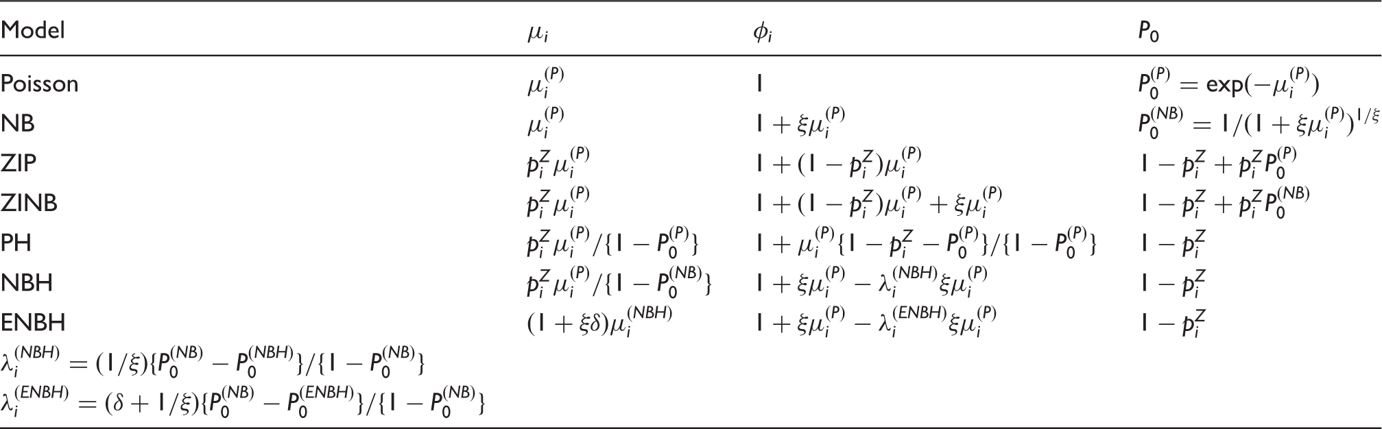
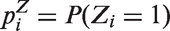
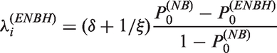
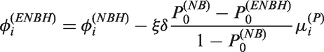
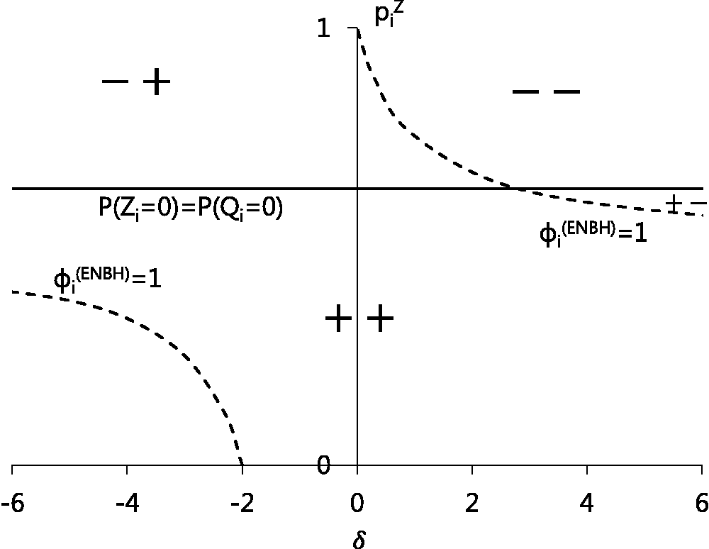
In Figure 3 at $μ_{i}^{(P)} = 1$ and ξ = 1, we plot curves for δ satisfying $φ_{i}^{(ENBH)} = 1$ in bold dashed lines and plot a line for $p_{i}^{Z}$ satisfying $P_{0}^{(ENBH)} = 1 - p_{i}^{Z} = P_{0}^{(P)} = exp (- μ_{i}^{(P)}) = 0.368$ in a bold line. From Figure 3, we see that in the ENBH model, all four combinations of {zero-inflation, zero-deflation} and {overdispersion, underdispersion} are possible as δ and $p_{i}^{Z}$ vary. Detailed explanation of Figure 3 is in the Supplementary material. Figure 4 plots probability functions in the next section of four combinations generated by the ENBH model at $μ_{i}^{(P)} = 1$ and ξ = 1.

Figure 3.

Region of generating zero-inflation (zero-deflation) with overdispersion (underdispersion) under the ENBH model. The solid line is $P (Z_{i} = 0) = P (Y_{i}^{(P)} = 0)$ and the dashed line is $φ_{i}^{(ENBH)} = 1$ .++, +–, –+ and – – represent regions for (zero-inflation, overdispersion), (zero-inflation, underdispersion), (zero-deflation, overderdispersion) and (zero-deflation, underdispersion), respectively.

Figure 4.

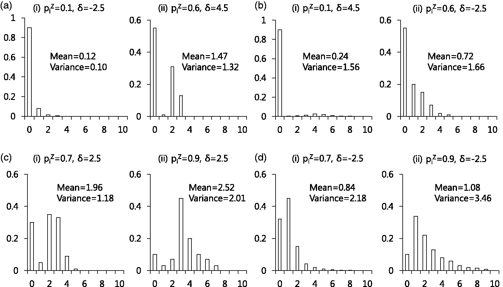
Distributions of ENBH when μ⁽ ^P ⁾= 1 and ξ = 1. (a) Zero - inflation with underdispersion, (b) Zero - inflation with overdispersion, (c) Zero - deflation with underdispersion, (d) Zero - deflation with overdispersion.

4.2 Estimating procedure

In this paper, we allow regression models for $μ_{i}^{(ENBH)}$ and $p_{i}^{Z}$ for the ith observation as follow

log (μ_{i}^{(ENBH)}) = X_{1 i}^{T} β_{1} and log {p_{i}^{Z} / ({1 - p}_{i}^{Z})} {= X}_{2 i}^{T} β_{2}

where

X_{1 i}

and

X_{2 i}

are model matrices for fixed effects β₁ and β₂. In the ENBH model with parameters

θ = (β_{1}^{T}, β_{2}^{T}, ξ, δ)^{T}

, the probability function of

Y_{i}^{(ENBH)}

has an explicit form

P_{0}^{(ENBH)} = P (Y_{i}^{(ENBH)} = 0; θ) = 1 - p_{i}^{Z}

and for

k = 1, 2, \dots

\begin{matrix} P (Y_{i}^{(ENBH)} = k; θ) = \int p_{i}^{Z} γ_{i} u_{i}^{δ} \frac{exp (- μ_{i}^{(P)} u_{i}) {μ_{i}^{(P)} u_{i}}^{k}}{k! P (N_{i} > 0)} f_{ξ} (u_{i}) d u_{i} \\ = (\begin{matrix} k + δ + 1 / ξ - 1 \\ 1 / ξ - 1 \end{matrix}) \times \frac{Γ (k + δ + 1) Γ (1 / ξ) p_{i}^{Z} {ξ μ_{i}^{(P)}}^{k}}{Γ (k + 1) Γ (δ + 1 / ξ) {(1 + ξ μ_{i}^{(P)})^{1 / ξ} - 1} (1 + μ_{i}^{(P)} ξ)^{k + δ}} \end{matrix}

For observed response data $y_{i} (k = 1, \dots, n)$ , the log-likelihood $\sum log L (θ; y_{i})$ can be explicitly formed by using the probability function of $Y_{i}^{(ENBH)}$ as follows

\sum log L (θ; y_{i}) = \sum log {P (Y_{i}^{(ENBH)} = y_{i}; θ)}

For estimation of β₁, we can use the chain rule

\sum d log L (θ; y_{i}) / d β_{1} = \sum (d log L (θ; y_{i}) / d μ_{i}^{(P)}) (d μ_{i}^{(P)} / d μ_{i}^{(ENBH)}) (d μ_{i}^{(ENBH)} / d β_{1})

where

d μ_{i}^{(P)} / d μ_{i}^{(ENBH)}

is obtained by using the equation

μ_{i}^{(ENBH)} = \frac{(1 + ξ δ) p_{i}^{Z} μ_{i}^{(P)}}{1 - 1 / (1 + ξ μ_{i}^{(P)})^{1 / ξ}}

We use the Newton–Raphson method to obtain the maximum likelihood estimators for θ.

5 Simulation study

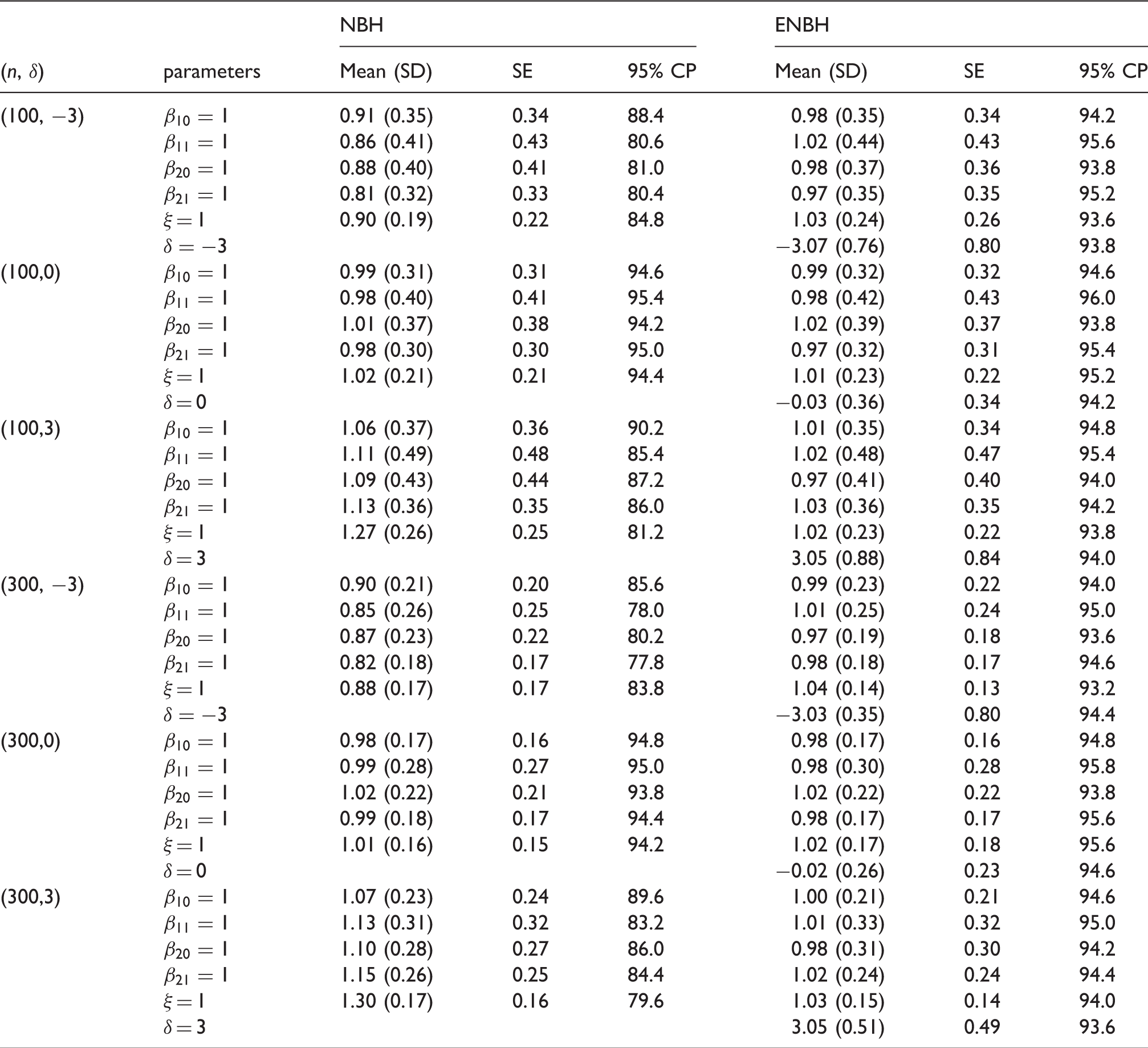
Numerical studies based upon 500 replications of simulated data are presented to evaluate the performance of the proposed methods. For the simulation study, we consider the ENBH model as follows

log (μ_{i}^{(ENBH)}) = β_{10} + β_{11} x_{1 i} and log {p_{i}^{Z} / (1 - p_{i}^{Z})} = β_{20} + β_{21} x_{2 i}

where x₁ _i and x₂ _i are independently generated N(0, 1), β₁₀ = β₁₁ = β₂₀ = β₂₁ = 1, ξ = 1 and δ = –3, 0, 3. For simulated data with sample size n = 100, 300, NBH and ENBH models are fitted. As shown in Table 6, we report the mean, the standard deviation (SD), the mean of the estimated standard error (SE) and the empirical coverage probability (CP) for a nominal 95% confidence interval (95%) for parameters.

Table 6.

Simulation results from NBH and ENBH models.

		NBH			ENBH
(n, δ)	parameters	Mean (SD)	SE	95% CP	Mean (SD)	SE	95% CP
(100, −3)	$β_{10} = 1$	0.91 (0.35)	0.34	88.4	0.98 (0.35)	0.34	94.2
	$β_{11} = 1$	0.86 (0.41)	0.43	80.6	1.02 (0.44)	0.43	95.6
	$β_{20} = 1$	0.88 (0.40)	0.41	81.0	0.98 (0.37)	0.36	93.8
	$β_{21} = 1$	0.81 (0.32)	0.33	80.4	0.97 (0.35)	0.35	95.2
	ξ = 1	0.90 (0.19)	0.22	84.8	1.03 (0.24)	0.26	93.6
	$δ = - 3$				−3.07 (0.76)	0.80	93.8
(100,0)	$β_{10} = 1$	0.99 (0.31)	0.31	94.6	0.99 (0.32)	0.32	94.6
	$β_{11} = 1$	0.98 (0.40)	0.41	95.4	0.98 (0.42)	0.43	96.0
	$β_{20} = 1$	1.01 (0.37)	0.38	94.2	1.02 (0.39)	0.37	93.8
	$β_{21} = 1$	0.98 (0.30)	0.30	95.0	0.97 (0.32)	0.31	95.4
	ξ = 1	1.02 (0.21)	0.21	94.4	1.01 (0.23)	0.22	95.2
	δ = 0				−0.03 (0.36)	0.34	94.2
(100,3)	$β_{10} = 1$	1.06 (0.37)	0.36	90.2	1.01 (0.35)	0.34	94.8
	$β_{11} = 1$	1.11 (0.49)	0.48	85.4	1.02 (0.48)	0.47	95.4
	$β_{20} = 1$	1.09 (0.43)	0.44	87.2	0.97 (0.41)	0.40	94.0
	$β_{21} = 1$	1.13 (0.36)	0.35	86.0	1.03 (0.36)	0.35	94.2
	ξ = 1	1.27 (0.26)	0.25	81.2	1.02 (0.23)	0.22	93.8
	δ = 3				3.05 (0.88)	0.84	94.0
(300, −3)	$β_{10} = 1$	0.90 (0.21)	0.20	85.6	0.99 (0.23)	0.22	94.0
	$β_{11} = 1$	0.85 (0.26)	0.25	78.0	1.01 (0.25)	0.24	95.0
	$β_{20} = 1$	0.87 (0.23)	0.22	80.2	0.97 (0.19)	0.18	93.6
	$β_{21} = 1$	0.82 (0.18)	0.17	77.8	0.98 (0.18)	0.17	94.6
	ξ = 1	0.88 (0.17)	0.17	83.8	1.04 (0.14)	0.13	93.2
	$δ = - 3$				−3.03 (0.35)	0.80	94.4
(300,0)	$β_{10} = 1$	0.98 (0.17)	0.16	94.8	0.98 (0.17)	0.16	94.8
	$β_{11} = 1$	0.99 (0.28)	0.27	95.0	0.98 (0.30)	0.28	95.8
	$β_{20} = 1$	1.02 (0.22)	0.21	93.8	1.02 (0.22)	0.22	93.8
	$β_{21} = 1$	0.99 (0.18)	0.17	94.4	0.98 (0.17)	0.17	95.6
	ξ = 1	1.01 (0.16)	0.15	94.2	1.02 (0.17)	0.18	95.6
	δ = 0				−0.02 (0.26)	0.23	94.6
(300,3)	$β_{10} = 1$	1.07 (0.23)	0.24	89.6	1.00 (0.21)	0.21	94.6
	$β_{11} = 1$	1.13 (0.31)	0.32	83.2	1.01 (0.33)	0.32	95.0
	$β_{20} = 1$	1.10 (0.28)	0.27	86.0	0.98 (0.31)	0.30	94.2
	$β_{21} = 1$	1.15 (0.26)	0.25	84.4	1.02 (0.24)	0.24	94.4
	ξ = 1	1.30 (0.17)	0.16	79.6	1.03 (0.15)	0.14	94.0
	δ = 3				3.05 (0.51)	0.49	93.6

NBH: NB hurdle; ENBH: extended NBH.

The NBH model gives very seriously biased estimators and their empirical coverage probabilities do not maintain the stated level when δ = –3 or 3. Estimators from the ENBH model seem to be consistent as sample size increased and confidence interval maintains the stated level. The standard-error estimates of ENBH estimators work well as judged by the very good agreement between SD and SE.

Supplemental Material

Supplemental material for Extended negative binomial hurdle models

Supplemental material for Extended negative binomial hurdle models by Maengseok Noh and Youngjo Lee in Statistical Methods in Medical Research

Footnotes

Declaration of conflicting interests

The author(s) declared no potential conflicts of interest with respect to the research, authorship, and/or publication of this article.

Funding

The author(s) disclosed receipt of the following financial support for the research, authorship, and/or publication of this article: This research was supported by the National Research Foundation of Korea (NRF) grant funded by Korea government (MEST) (grant no. 2011-0030810, 2013R1A1A1012710) and the Brain Research Program through the NRF funded by the Ministry of Science, ICT and Future Planning (grant no. 2014M3C7A1062896).

Supplemental material

Supplemental material for this article is available online.

References

Johnson

Kotz

Kemp

. Univariate discrete distributions, 2nd ed. New York, NY: Wiley, 1992.

Morgan

. Some stochastic models to describe the fertilization of an egg. Appl Stat 1975; 24: 137–138.

Morgan

BJT

. Modelling polyspermy. Biometrics 1982; 38: 885–898.

Daley

Maindonald

. A unified view of models describing the avoidance of superparasitism. IMA J Math App Biol Med 1989; 6: 161–178.

Griffiths

. Avoidance-modified generalised distributions and their application to studies of superparasitism. Biometrics 1977; 33: 103–112.

Singh

. A note on inflated Poisson distribution. J Ind Statist Assoc 1963; 1: 140–144.

Lambert

. Zero-inflated Poisson regression with an application to defects in manufacturing. Technometrics 1992; 34: 1–14.

Cragg

. Some statistical models for limited dependent variables with application to the demand for durable goods. Econometrica 1971; 39: 829–844.

Mullahy

. Specification and testing of some modified count data models. J Econom 1986; 33: 341–365.

10.

Lee

Alam

Noh

et al.

Spatial model with excessive zero counts for analysis of the changes in reindeer distribution. Ecol Evol 2016; 6: 7047–7056.

11.

Lee

Nelder

. Hierarchical generalized linear models. J R Statist Soc B 1996; 58: 619–678.

12.

Chernyavskiy

Little

Rosenberg

. Correlated Poisson models for age-period-cohort analysis. Stat Med 2018; 37: 405–424.

13.

Moloas

Lesaffre

. Hurdle models for multilevel zero-inflated data via h-likelihood. Stat Med 2010; 29: 3294–3310.

14.

Tin A. Modeling zero-inflated count data with underdispersion and overdispersion. SAS Global Forum, Statistics and Data Analysis 2008

15.

Lee Y, Nelder JA and Pawitan Y. Generalized linear models with random effects, unified analysis via H-likelihood. 2nd ed. London: Chapman & Hall/CRC, 2017

16.

Deb

Trivedi

. Demand for medical care by the elderly: a finite mixture approach. J Appl Econom 1997; 12: 313–326.

17.

Zorn

CJW

. Evaluating zero-inflated and hurdle Poisson specifications. Midw Polit Sci Assoc 1996, pp. 1–16.

Supplementary Material

Please find the following supplemental material available below.

For Open Access articles published under a Creative Commons License, all supplemental material carries the same license as the article it is associated with.

For non-Open Access articles published, all supplemental material carries a non-exclusive license, and permission requests for re-use of supplemental material or any part of supplemental material shall be sent directly to the copyright owner as specified in the copyright notice associated with the article.

0.00 MB

0.21 MB