In medical diagnostic studies, a diagnostic test can be evaluated based on its sensitivity under a desired specificity. Existing methods for inference on sensitivity include normal approximation-based approaches and empirical likelihood (EL)-based approaches. These methods generally have poor performance when the specificity is high, and some require choosing smoothing parameters. We propose a new influence function-based empirical likelihood method and Bayesian empirical likelihood methods to overcome such problems. Numerical studies are performed to compare the finite sample performance of the proposed approaches with existing methods. The proposed methods are shown to perform better in terms of both coverage probability and interval length. A real data set from Alzheimer’s Disease Neuroimaging Initiative (ANDI) is analyzed.
Over the past 100 years, diagnostic testing has become a critical part of standard medical practice.1 Diagnostic tests commonly measure different biomarkers of a subject in question, and the disease status of the subject is determined based on whether such measurements meet pre-specified criteria. For many tests, the clinicians would identify the subject as diseased if test result is above a certain cutoff and non-diseased if it is below the cutoff (or vice-versa). For example, hypertension is defined as a systolic blood pressure above 120 mmHg and diastolic blood pressure above 80 mmHg.
The accuracy of a diagnostic test is commonly evaluated based on its sensitivity and specificity, i.e. the probabilities of correct diagnoses for diseased subjects and for non-diseased subjects, respectively. Both sensitivity and specificity are not fixed but depend on the cutoff(s) chosen for that test. The receiver operating characteristic (ROC) curve of a test is constructed to show how sensitivity and specificity change as the cutoff varies. Different statistics including the area under the ROC curve (AUC)2 and Youden index3 are based on the ROC curve. They are used to evaluate the discriminatory ability of diagnostic tests. In practice, however, the cutoff of a test is usually chosen so that the specificity is meaningfully high.4 For example, recent breast MRI screening study results usually have specificity of at least 80%.5 In this paper, we focus on interval estimation of the sensitivity at a certain specificity.
Existing methods for interval estimation of sensitivity include normal approximation-based approaches and empirical likelihood-based approaches. Linnet6 proposed a normal approximation (NA)-based confidence interval. Platt et al.4 noted that Linnet’s method may be greatly affected by poor empirical density estimation, and proposed to use Efron’s bias-corrected acceleration (BCa) bootstrap interval.7 Zhou and Qin8 developed two bootstrap intervals for sensitivity based on extensions of Agresti and Coull’s results on confidence intervals for binomial proportions,9 and showed that the new bootstrap intervals have better coverage accuracy than the NA and BCa intervals. Empirical likelihood (EL), introduced by Owen,10 has become a popular approach in statistical research because it does not rely on parametric assumptions on the data but still enjoys the advantages of likelihood methods. In particular, EL methods have been used widely in evaluation of diagnostic tests. For example, Gong et al.11 proposed a smoothed jackknife empirical likelihood (JEL) method for the ROC curve. Qin et al.12 developed a hybrid EL (HEL) method for sensitivity.
In this article, we provide a thorough review of these methods and comprehensive numerical studies to compare their performance in different settings. Moreover, we study two improvements of current methods. First, we note that in the approach of Qin et al.,12 the hybrid empirical likelihood ratio follows a scaled chi-square distribution asymptotically, thus an extra step is required to estimate this scale. We propose a new influence function-based EL (IFEL) method following Yu et al.13 The idea is to replace the estimating function in the EL with an influence function of the sensitivity. The corresponding empirical log-likelihood ratio statistic converges to a standard chi-square distribution, which makes inference for sensitivity more convenient. Second, we develop Bayesian empirical likelihood (BEL) approaches. Despite the extensive use in the frequentist context, EL has only recently been used in Bayesian analysis. Lazar14 observed that the properties of EL are in many respects similar to those of parametric likelihoods, and EL could be used in Bayesian inference like parametric likelihoods. To our knowledge, Bayesian EL methods have not been used in evaluating diagnostic tests. We propose to apply Bayesian EL methods to the inference of sensitivity. A critical part of Bayesian approaches is choosing an appropriate prior, which becomes quite tricky since no parametric model is assumed for EL. We consider building EL and assigning priors on either the sensitivity parameter itself or the probability vector in building EL. For EL on the sensitivity parameter, we follow Clarke and Yuan15 to derive reference priors.16–18 In addition, we apply the idea of Rao and Wu19 to employ Bayesian EL based on .
The article is organized as follows. In Section 2, we review several existing methods for interval estimation of sensitivity. In Section 3, we introduce a new EL ratio statistic for sensitivity based on influence function. In Section 4, we propose Bayesian EL methods based on influence function and hybrid methods. In Section 5, we conduct simulation studies to compare the performance of the proposed methods with existing methods. In Section 6, we apply the new methods to a real dataset to assess the diagnostic accuracy of three biomarkers in the detection of Alzheimer’s disease. A sample R code for the implementation of the proposed methods is provided in Appendix 2.
2 Existing methods of constructing confidence intervals for sensitivity
Let Y and X be results from a continuous-scale test for diseased and non-diseased subjects, respectively. Suppose subjects are diagnosed as diseased if the results are greater than a cutoff η, and non-diseased if the results are below η. The sensitivity and specificity of this test are defined by
where G and F are the distribution functions of Y and X, respectively. Therefore, when the specificity of the test is p (), the corresponding sensitivity is . Let and be the test results of a random sample of diseased subjects and non-diseased subjects, respectively. The statistical problem is to construct confidence intervals for the sensitivity θ at a fixed specificity p based on these observations.
2.1 Normal approximation-based bootstrap methods
As mentioned in introduction section, Zhou and Qin8 developed two bootstrap intervals for the sensitivity which have better coverage accuracy than other normal-approximation based confidence intervals. Their methods used Agresti and Coull’s idea for construction of confidence interval of a binomial proportion.9 The first confidence interval, called bootstrap I (BTI) interval, for θ is defined by
where
is the p-th quantile of is the empirical distribution function of F, is the -th quantile of the standard normal distribution, and the variance of is estimated by the following bootstrap procedure:
Draw a resample 's of size n and a separate resample 's of size m with replacement, from the diseased sample Yj’s and the non-diseased sample Xi’s, respectively.
Calculate the bootstrap version of
where is the p-th sample quantile based on the bootstrap resample 's.
Repeat the first two steps B times ( is recommended) to obtain a set of bootstrap replications . Then, the bootstrap variance estimator is defined by
where .
The second confidence interval, called bootstrap II (BTII) interval, for θ is defined by
BTI and BTII intervals are shown to have better coverage accuracy and shorter interval lengths than the normal approximation-based interval and the BCa interval regardless of the sample sizes and for both normal and non-normal data when specificity p is high. However, the coverage accuracy usually deteriorates for small sample sizes.
2.2 Jackknife empirical likelihood (JEL) method
Motivated by the JEL method for a U-statistic,20 Gong et al.11 proposed a smoothed jackknife method by applying the standard EL method to the jackknife sample mean. A simple empirical estimator for θ is defined as
where is the empirical distribution functions of G.
where , w is a symmetric density function with support , and is a bandwidth.
Let
and
where
The jackknife pseudo-sample is then defined as
and the JEL for the sensitivity θ is defined as
By standard Lagrange multiplier arguments, the empirical log-likelihood ratio can be derived as
where λ satisfies
Gong et al.11 showed that converges in distribution to the standard chi-square distribution with one degree of freedom, and a level JEL-based confidence interval on θ is given by
where is the -th quantile of . As previously mentioned, JEL method needs to choose a bandwidth for kernel estimation.
2.3 Hybrid empirical likelihood method
A challenge in constructing confidence intervals for sensitivity is to estimate the cut-off point that yields the desired specificity. Qin et al.12 proposed a hybrid EL-based procedure which does not estimate an explicit cut-off point.
For a test value Y from a diseased subject, let . U is called the placement value of Y and can be interpreted as the proportion of the non-diseased population with test value greater than Y. It essentially marks the placement of Y within the non-diseased distribution.21 We have
Based on this relationship between θ and U
can be used in EL as the estimating function. Qin et al.12 proposed a profile EL which replaces F with the corresponding empirical distribution function as follow
where with for . The corresponding empirical log-likelihood ratio is
where is the solution of
The asymptotic distribution of is a scaled chi-squared distribution with one degree of freedom. Thus, a level hybrid EL and bootstrap confidence interval for θ can be constructed as follows
where can be estimated from the following bootstrap procedure:
Draw a resample 's of size n and a separate resample 's of size m with replacement, from the diseased sample Yj’s and the non-diseased sample Xi’s, respectively.
Calculate the bootstrap estimator of θ
where is the p-th sample quantile based on the bootstrap resample 's.
Repeat the first two steps B times to obtain a set of bootstrap replications . Then is defined by
where .
Qin et al.12 showed that this hybrid empirical likelihood (HEL) interval has good coverage probability when sample size is greater than (50, 50). However, estimating could be computationally expensive and not desirable.
Yu et al.13 proposed an EL function based on influence functions of parameters of interest. Motivated by their study, we propose a new influence function-based EL method to construct confidence intervals for sensitivity. Recall that , and . Denote (i.e. the p-th sample quantile of Xi’s), and the combined samples as
We have the following decomposition
with
From the Bahadur representation for the sample quantile 22
It follows that
where f and g are the densities for X and Y, respectively.
Therefore
where
is called the influence function of θ.
From equation (6), we can easily get the following asymptotic distribution of the empirical estimator for θ.
Proposition 1
Assume that F and G are continuous distribution functions with density functions f and g, respectively, is strictly positive, and are bounded in a neighborhood of . If (), then
where
Linnet6 heuristically derived the conclusion in Proposition 1, but he did not explicitly give the formula for the asymptotic variance (see Zhou and Qin8).
Based on the influence function, an EL for the sensitivity θ can be defined as follows
where is the estimated influence function of θ given as follows
where and are the density estimators for g and f, respectively.
Here we use the following kernel estimator for f
where is a Gaussian kernel function, and the bandwidth is the “rule-of-thumb” bandwidth23 defined by
where sX and iqrX are, respectively, the standard deviation and the inter-quartile range, of the sample Xi’s. The above bandwidth is also adopted by Zou et al.24
The density function g can be estimated similarly. When f and g are uniformly continuous, the kernel estimators and defined above are almost surely and uniformly consistent.25
By the Lagrange multiplier, the maximization of equation (9) is achieved at
where λ is the solution of
The corresponding empirical log-likelihood ratio statistic is
When test results Yk’s are not all greater/smaller than , the empirical log-likelihood ratio is well defined on (0, 1). The following theorem establishes the asymptotic distribution of and the proof is given in Appendix 1.
Theorem 1
Assume that F and G are distribution functions with uniformly continuous density functions f and g, respectively, is strictly positive, , and are bounded in a neighborhood of . If θ0 is the true value of the sensitivity at a fixed level p of specificity, and (), then the limiting distribution of is a standard chi-squared distribution with one degree of freedom as .
From Theorem 1, a level influence function-based EL confidence interval for θ can be constructed as
4 Bayesian empirical likelihood method
Lazar14 noted that EL has many of the same asymptotic properties as those derived from parametric models. In this sense, EL could be used as the basis for Bayesian inference. Conceptually, Bayesian EL enjoys the advantages of both EL and Bayesian methods: (i) no parametric assumption is needed by incorporating EL; (ii) Bayesian framework quantifies uncertainty more naturally, and with proper choices of priors, the Bayesian EL methods can outperform the classical EL methods.26 We propose two types of Bayesian EL methods to construct credible intervals for sensitivity.
4.1 Bayesian empirical likelihood based on sensitivity
We noticed that the classical EL intervals (e.g. HEL and JEL) for sensitivity at a high specificity level (e.g. p = 0.95) sometimes have under-coverage problems with small sample sizes (e.g. . See section 5). With prior knowledge on the diagnostic accuracy (i.e. sensitivity/specificity) of a test, Bayesian EL methods could improve small sample performances of the classical EL methods, which motivated us propose Bayesian EL methods for inference in medical diagnostics. To our knowledge, this article is the first application of Bayesian EL in medical diagnostics. We follow Lazar14 to combine empirical likelihood with a specified prior on θ via the Bayes theorem to obtain a posterior
Instead of using parametric likelihood in traditional Bayesian framework, we use empirical likelihood here. An important step is to choose an appropriate prior on sensitivity θ. We consider reference priors in this study. Reference priors, originally introduced by Bernardo,16 and further developed by Berger et al.,17,18 are a popular choice for objective priors. They are an important type of objective priors which only depend on the assumed model and the available data. In our problem, since we do not have a parametric model, we follow Clarke and Yuan15 to derive reference priors for EL. The following proposition gives the reference priors for the Bayesian hybrid EL method where is used as the likelihood, and and are defined in equations (3) and (5) from section 2.3.
Proposition 2
The reference prior based on the relative entropy for HEL using from equation (2) is
and the reference prior based on Hellinger distance is
where is the beta distribution with parameters a and b. The corresponding posterior is
Based on these posteriors, we can calculate two equal-tail credible intervals for θ. We call them as the Bayesian Hybrid Empirical Likelihood 1 (BHEL1) interval and the Bayesian Hybrid Empirical Likelihood 2 (BHEL2) interval using priors and , respectively.
Similarly, to construct Bayesian credible intervals for θ based on the IFEL using in equation (7), we propose the following reference priors
and
These two priors are both proper since is bounded by a constant and is bounded by a beta distribution. In practice, we use to estimate the influence function , and replace f, g, and η with their estimates since they are generally unknown. The posterior based on this approach is then
where .
Based on these posteriors, we also can calculate two equal-tail credible intervals for θ. We call them as Bayesian Influence Function-based Empirical Likelihood 1 (BIFEL1) and Bayesian Influence Function-based Empirical Likelihood 2 (BIFEL2) intervals using priors and , respectively.
4.2 Bayesian pseudo empirical likelihood (BpEL) based on probability vector
The methods presented in section 4.1 are based on the posterior distributions of θ. In this section, instead of applying priors on θ, we apply Rao and Wu’s method19 to obtain an alternative approach for Bayesian EL inference on θ based on probability vector . We treat as unknown parameters and the EL function is
where l = n for hybrid EL, and for influence function EL. Consider the Dirichlet prior on
where . The posterior distribution of given the data is Dirichlet is given by
The posterior of sensitivity θ satisfies the following equation
where is an estimating/influence function and follows the Dirichlet distribution . In practice, we can generate samples of from , and by solving equation (12), we get the posterior samples of θ. Based on these posterior samples, we can calculate the equal-tail credible intervals for sensitivity θ.
Similar to section 4.1, we consider two types of EL: hybrid EL (equation (3)) and influence function EL (equation (9)). We call them Bayesian pseudo hybrid EL (BpHEL) and Bayesian pseudo influence function EL (BpIFEL), respectively. For BpHEL, we use to replace in equation (12), and consider and as the priors (labeled BpHEL1 and BpHEL2, respectively), where is the scale estimate defined in Section 2.32. For BpIFEL, similarly, we use to replace in equation (12), and consider and as the priors (labeled BpIFEL1 and BpIFEL2, respectively).
5 Simulation study
Simulation studies are conducted to examine the finite sample performance of the proposed approaches: influence function-based empirical likelihood (IFEL), Bayesian influence function empirical likelihood methods (BIFEL1 and BIFEL2) with reference priors and , Bayesian hybrid empirical likelihood methods (BHEL1 and BHEL2) with reference priors and , Bayesian pseudo influence function empirical likelihood method (BpIFEL), and Bayesian pseudo hybrid empirical likelihood method (BpHEL). We compare them with existing approaches including BTI, BTII, smoothed JEL method, hybrid empirical likelihood method (HEL), and the modified normal approximation (NA) method proposed by Linnet.6
5.1 Simulation settings
We consider seven simulation settings for the underlying non-diseased distribution F and diseased distribution G: (i) Normal distributions with and , (ii) normal distributions with and , (iii) normal distributions with and , (iv) exponential distributions with and , (v) exponential distributions with and , (vi) mixed distributions with and , and (vii) mixed distributions with and . Under settings (i), (ii) and (iii), both the diseased and non-diseased distributions of test results are normal distributions but with different degrees of separation and corresponding to low, medium, and high sensitivity, respectively. Similarly, settings (iv), (vi) and settings (v), (vii) are corresponding to medium and high sensitivity, respectively. Random samples of size m and n are generated from F and G, respectively. Sample sizes (m, n) = (20, 20), (50, 50), (100, 100), (50, 100), (100, 50), (500, 500) are considered. We construct 95% level confidence (credible) intervals for sensitivity θ at specificity levels , 90% and 95%, respectively. The simulation procedure is repeated 5000 times to find the frequentist coverage probabilities and average lengths of the intervals. For JEL method, we use the kernel and as suggested by Gong et al.11
5.2 Simulation results
The simulation results under the normal distribution settings are reported in Tables 1
Coverage probabilities and average lengths of 95% confidence intervals for sensitivity θ at a fixed level of specificity p when and .
p = 0.95,
p = 0.90,
p = 0.80,
Coverage
Average
Coverage
Average
Coverage
Average
(m,n)
Methods
Probability
Length
Probability
Length
Probability
Length
(20,20)
NA
0.821
0.539
0.865
0.597
0.898
0.603
BTI
0.817
0.596
0.874
0.609
0.898
0.573
BTII
0.809
0.596
0.884
0.609
0.918
0.573
JEL
0.901
0.314
0.892
0.378
0.906
0.456
HEL
0.829
0.540
0.932
0.574
0.953
0.547
BHEL1
0.842
0.521
0.939
0.529
0.972
0.509
BHEL2
0.855
0.552
0.919
0.566
0.955
0.539
BpHEL1
0.856
0.553
0.909
0.582
0.932
0.553
BpHEL2
0.837
0.525
0.896
0.553
0.916
0.528
IFEL
0.820
0.485
0.902
0.594
0.924
0.614
BIFEL1
0.819
0.457
0.909
0.560
0.951
0.594
BIFEL2
0.822
0.465
0.900
0.581
0.932
0.620
BpIFEL1
0.836
0.571
0.877
0.625
0.919
0.625
BpIFEL2
0.837
0.564
0.873
0.616
0.914
0.618
(50,50)
NA
0.874
0.379
0.902
0.405
0.921
0.394
BTI
0.901
0.425
0.918
0.435
0.927
0.401
BTII
0.901
0.425
0.931
0.435
0.940
0.401
JEL
0.931
0.236
0.879
0.288
0.922
0.332
HEL
0.888
0.384
0.944
0.423
0.951
0.395
BHEL1
0.926
0.386
0.945
0.400
0.964
0.375
BHEL2
0.943
0.392
0.945
0.414
0.963
0.393
BpHEL1
0.943
0.390
0.942
0.422
0.960
0.401
BpHEL2
0.923
0.378
0.936
0.411
0.956
0.391
IFEL
0.915
0.388
0.919
0.422
0.933
0.405
BIFEL1
0.915
0.364
0.934
0.414
0.951
0.408
BIFEL2
0.912
0.370
0.931
0.426
0.944
0.417
BpIFEL1
0.893
0.401
0.901
0.405
0.924
0.391
BpIFEL2
0.902
0.407
0.913
0.414
0.940
0.402
(100,100)
NA
0.899
0.277
0.921
0.294
0.934
0.284
BTI
0.929
0.318
0.935
0.317
0.941
0.293
BTII
0.944
0.318
0.944
0.317
0.952
0.293
JEL
0.907
0.183
0.865
0.224
0.931
0.249
HEL
0.934
0.309
0.943
0.314
0.953
0.290
BHEL1
0.927
0.304
0.947
0.304
0.954
0.283
BHEL2
0.935
0.310
0.945
0.312
0.954
0.287
BpHEL1
0.934
0.312
0.942
0.316
0.955
0.291
BpHEL2
0.933
0.306
0.943
0.311
0.948
0.287
IFEL
0.915
0.291
0.933
0.304
0.940
0.288
BIFEL1
0.907
0.284
0.940
0.306
0.950
0.287
BIFEL2
0.907
0.289
0.937
0.311
0.944
0.290
BpIFEL1
0.902
0.281
0.925
0.296
0.934
0.284
BpIFEL2
0.898
0.285
0.932
0.299
0.943
0.285
(500, 500)
NA
0.933
0.132
0.933
0.137
0.951
0.129
BTI
0.944
0.145
0.944
0.145
0.944
0.145
BTII
0.952
0.145
0.952
0.145
0.952
0.145
JEL
0.937
0.139
0.938
0.113
0.942
0.139
HEL
0.947
0.145
0.944
0.144
0.956
0.133
BHEL1
0.944
0.144
0.943
0.143
0.957
0.132
BHEL2
0.947
0.144
0.944
0.144
0.956
0.133
BpHEL1
0.937
0.144
0.934
0.145
0.961
0.133
BpHEL2
0.936
0.144
0.931
0.144
0.958
0.132
IFEL
0.934
0.134
0.935
0.138
0.951
0.129
BIFEL1
0.938
0.136
0.939
0.139
0.953
0.130
BIFEL2
0.941
0.137
0.941
0.139
0.952
0.130
BpIFEL1
0.928
0.135
0.939
0.138
0.954
0.130
BpIFEL2
0.926
0.134
0.941
0.138
0.950
0.130
(50,100)
NA
0.857
0.335
0.892
0.359
0.924
0.349
BTI
0.896
0.389
0.919
0.394
0.932
0.359
BTII
0.903
0.389
0.928
0.394
0.941
0.359
JEL
0.872
0.216
0.857
0.284
0.919
0.313
HEL
0.897
0.357
0.929
0.384
0.938
0.350
BHEL1
0.910
0.351
0.931
0.363
0.952
0.337
BHEL2
0.917
0.358
0.934
0.379
0.954
0.346
BpHEL1
0.917
0.357
0.928
0.386
0.948
0.351
BpHEL2
0.906
0.348
0.925
0.377
0.944
0.345
IFEL
0.893
0.337
0.912
0.378
0.931
0.360
BIFEL1
0.867
0.310
0.917
0.366
0.948
0.362
BIFEL2
0.864
0.310
0.914
0.369
0.943
0.366
BpIFEL1
0.882
0.370
0.909
0.370
0.937
0.352
BpIFEL2
0.883
0.369
0.907
0.368
0.936
0.351
(100,50)
NA
0.911
0.326
0.922
0.349
0.930
0.341
BTI
0.924
0.358
0.919
0.366
0.935
0.345
BTII
0.932
0.358
0.932
0.366
0.944
0.345
JEL
0.943
0.196
0.875
0.237
0.924
0.283
HEL
0.928
0.350
0.952
0.366
0.955
0.345
BHEL1
0.937
0.344
0.953
0.349
0.960
0.333
BHEL2
0.942
0.351
0.949
0.361
0.952
0.342
BpHEL1
0.940
0.352
0.951
0.367
0.952
0.347
BpHEL2
0.933
0.344
0.949
0.359
0.951
0.342
IFEL
0.924
0.336
0.933
0.357
0.941
0.343
BIFEL1
0.927
0.328
0.950
0.355
0.959
0.341
BIFEL2
0.933
0.337
0.948
0.365
0.952
0.348
BpIFEL1
0.916
0.334
0.940
0.356
0.947
0.344
BpIFEL2
0.912
0.333
0.941
0.354
0.946
0.343
to 3. From Table 1 where the sensitivity is at low level, we observe that HEL and Bayesian approaches based on HEL have the best overall performance. Bayesian approaches generally have similar or improved performance over HEL. We note that BpHEL2 intervals generally have lower coverage probabilities than the three other Bayesian HEL intervals when sample size is (20, 20). The possible reason is the modified prior is not good for small sample size. IFEL and corresponding Bayesian approaches have slightly worse performance compared with HEL-related approaches, especially when specificity is high.
BTI and BTII are generally not as good, especially when sample size is small. JEL performs the best under one setting (when sample size is (20, 20) and specificity ) but has poor performance compared with our methods for other settings. Under the unbalanced sample setting, our new methods are similar to or better than others, and BHEL and BpHEL methods are much better than HEL. We also notice that the performance for sample size (100, 50) is much better than that of sample size (50, 100). It indicates that non-diseased samples are more important in the inference of sensitivity with high specificity. Comparing the results from the normal distribution setting (i) with those from the normal distribution settings (ii) and (iii) which have higher degree of separation and higher sensitivity, we can see from Tables 2
Coverage probabilities and average lengths of 95% confidence intervals for sensitivity θ at a fixed level of specificity p when and .
p = 0.95,
p = 0.90,
p = 0.80,
Coverage
Average
Coverage
Average
Coverage
Average
(m,n)
Methods
Probability
Length
Probability
Length
Probability
Length
(20, 20)
NA
0.768
0.534
0.853
0.480
0.868
0.363
BTI
0.779
0.558
0.860
0.496
0.903
0.359
BTII
0.784
0.558
0.877
0.496
0.913
0.359
JEL
0.783
0.236
0.800
0.260
0.748
0.270
HEL
0.826
0.500
0.819
0.389
0.563
0.225
BHEL1
0.933
0.475
0.935
0.411
0.947
0.224
BHEL2
0.890
0.523
0.928
0.482
0.820
0.388
BpHEL1
0.858
0.527
0.926
0.466
0.854
0.305
BpHEL2
0.834
0.498
0.918
0.441
0.854
0.292
IFEL
0.768
0.428
0.876
0.443
0.833
0.313
BIFEL1
0.845
0.398
0.858
0.433
0.899
0.257
BIFEL2
0.835
0.456
0.857
0.450
0.893
0.121
BpIFEL1
0.797
0.546
0.859
0.497
0.876
0.363
BpIFEL2
0.783
0.539
0.858
0.491
0.871
0.358
(50, 50)
NA
0.857
0.402
0.887
0.335
0.910
0.240
BTI
0.888
0.456
0.910
0.363
0.918
0.245
BTII
0.902
0.456
0.923
0.363
0.929
0.245
JEL
0.820
0.205
0.888
0.230
0.884
0.217
HEL
0.955
0.445
0.943
0.345
0.878
0.203
BHEL1
0.951
0.418
0.967
0.348
0.947
0.248
BHEL2
0.940
0.437
0.955
0.351
0.960
0.245
BpHEL1
0.932
0.446
0.942
0.350
0.944
0.235
BpHEL2
0.920
0.431
0.932
0.340
0.936
0.231
IFEL
0.891
0.433
0.916
0.343
0.923
0.232
BIFEL1
0.902
0.405
0.945
0.353
0.923
0.240
BIFEL2
0.889
0.410
0.935
0.355
0.930
0.196
BpIFEL1
0.897
0.441
0.928
0.348
0.941
0.245
BpIFEL2
0.892
0.439
0.925
0.346
0.938
0.244
(100, 100)
NA
0.883
0.305
0.914
0.246
0.934
0.173
BTI
0.917
0.352
0.930
0.264
0.937
0.176
BTII
0.929
0.352
0.940
0.264
0.946
0.176
JEL
0.905
0.150
0.842
0.191
0.903
0.158
HEL
0.935
0.344
0.953
0.262
0.936
0.169
BHEL1
0.956
0.330
0.959
0.259
0.959
0.181
BHEL2
0.944
0.340
0.950
0.260
0.960
0.176
BpHEL1
0.926
0.341
0.946
0.258
0.958
0.173
BpHEL2
0.918
0.335
0.936
0.255
0.954
0.171
IFEL
0.904
0.314
0.927
0.250
0.947
0.174
BIFEL1
0.907
0.314
0.937
0.256
0.953
0.174
BIFEL2
0.902
0.316
0.929
0.257
0.954
0.174
BpIFEL1
0.897
0.314
0.927
0.251
0.943
0.174
BpIFEL2
0.897
0.313
0.926
0.250
0.944
0.173
(500, 500)
NA
0.921
0.149
0.938
0.115
0.950
0.078
BTI
0.948
0.165
0.944
0.120
0.947
0.078
BTII
0.953
0.165
0.950
0.120
0.955
0.078
JEL
0.940
0.236
0.930
0.233
0.932
0.212
HEL
0.953
0.163
0.950
0.120
0.949
0.078
BHEL1
0.955
0.162
0.952
0.120
0.954
0.079
BHEL2
0.954
0.163
0.950
0.120
0.955
0.078
BpHEL1
0.958
0.163
0.944
0.120
0.936
0.078
BpHEL2
0.958
0.162
0.948
0.120
0.932
0.078
IFEL
0.931
0.150
0.942
0.115
0.951
0.078
BIFEL1
0.937
0.153
0.950
0.116
0.949
0.078
BIFEL2
0.936
0.153
0.950
0.116
0.948
0.078
BpIFEL1
0.933
0.152
0.946
0.116
0.944
0.078
BpIFEL2
0.939
0.151
0.944
0.116
0.945
0.078
(50, 100)
NA
0.834
0.363
0.879
0.295
0.917
0.206
BTI
0.882
0.421
0.912
0.328
0.931
0.213
BTII
0.890
0.421
0.924
0.328
0.941
0.213
JEL
0.894
0.188
0.927
0.221
0.909
0.195
HEL
0.927
0.408
0.934
0.315
0.911
0.190
BHEL1
0.935
0.384
0.953
0.312
0.955
0.218
BHEL2
0.922
0.400
0.943
0.314
0.956
0.209
BpHEL1
0.910
0.406
0.934
0.312
0.946
0.201
BpHEL2
0.900
0.394
0.928
0.305
0.944
0.198
IFEL
0.870
0.367
0.910
0.307
0.936
0.208
BIFEL1
0.845
0.338
0.927
0.302
0.942
0.211
BIFEL2
0.840
0.340
0.915
0.303
0.945
0.209
BpIFEL1
0.877
0.400
0.918
0.305
0.944
0.209
BpIFEL2
0.880
0.399
0.919
0.303
0.944
0.208
(100, 50)
NA
0.893
0.354
0.921
0.295
0.922
0.213
BTI
0.916
0.393
0.926
0.308
0.926
0.214
BTII
0.929
0.393
0.936
0.308
0.931
0.214
JEL
0.911
0.172
0.921
0.200
0.922
0.187
HEL
0.960
0.388
0.958
0.307
0.913
0.193
BHEL1
0.964
0.369
0.959
0.304
0.952
0.224
BHEL2
0.953
0.382
0.955
0.305
0.963
0.218
BpHEL1
0.952
0.387
0.950
0.307
0.954
0.211
BpHEL2
0.946
0.377
0.940
0.301
0.952
0.208
IFEL
0.907
0.363
0.932
0.295
0.925
0.208
BIFEL1
0.932
0.372
0.950
0.302
0.922
0.211
BIFEL2
0.928
0.378
0.945
0.304
0.934
0.174
BpIFEL1
0.916
0.365
0.940
0.300
0.940
0.214
BpIFEL2
0.919
0.363
0.936
0.299
0.939
0.213
Coverage probabilities and average lengths of 95% confidence intervals for sensitivity θ at a fixed level of specificity p when and .
p = 0.95,
p = 0.90,
p = 0.80,
Coverage
Average
Coverage
Average
Coverage
Average
(m,n)
Methods
Probability
Length
Probability
Length
Probability
Length
(20, 20)
NA
0.765
0.292
0.892
0.267
0.827
0.268
BT1
0.820
0.307
0.908
0.281
0.849
0.234
BT2
0.838
0.307
0.897
0.281
0.864
0.234
JEL
0.821
0.282
0.797
0.225
0.785
0.220
HEL
0.747
0.287
0.751
0.239
0.805
0.178
BHEL1
0.963
0.352
0.963
0.338
0.944
0.312
BHEL2
0.969
0.338
0.968
0.318
0.964
0.287
BpHEL1
0.928
0.303
0.910
0.268
0.912
0.216
BpHEL2
0.923
0.294
0.908
0.261
0.891
0.211
IF
0.848
0.259
0.854
0.221
0.882
0.165
BIFEL1
0.844
0.364
0.898
0.368
0.878
0.222
BIFEL2
0.887
0.367
0.849
0.373
0.895
0.182
BpIF1
0.926
0.278
0.892
0.251
0.886
0.211
BpIF2
0.924
0.275
0.890
0.248
0.812
0.209
(50, 50)
NA
0.868
0.119
0.882
0.185
0.869
0.157
BT1
0.901
0.225
0.906
0.197
0.925
0.166
BT2
0.915
0.225
0.904
0.197
0.911
0.166
JEL
0.782
0.213
0.802
0.195
0.892
0.160
HEL
0.929
0.233
0.923
0.194
0.909
0.151
BHEL1
0.954
0.238
0.959
0.210
0.956
0.185
BHEL2
0.951
0.234
0.955
0.202
0.968
0.173
BpHEL1
0.943
0.230
0.939
0.196
0.933
0.164
BpHEL2
0.942
0.228
0.936
0.194
0.924
0.161
IF
0.915
0.220
0.918
0.172
0.916
0.139
BIFEL1
0.900
0.140
0.916
0.125
0.909
0.070
BIFEL2
0.915
0.950
0.895
0.129
0.901
0.107
BpIF1
0.915
0.394
0.919
0.179
0.918
0.152
BpIF2
0.915
0.338
0.919
0.178
0.918
0.152
(100, 100)
NA
0.902
0.153
0.902
0.135
0.915
0.113
BT1
0.918
0.167
0.924
0.144
0.921
0.119
BT2
0.914
0.167
0.927
0.144
0.923
0.119
JEL
0.842
0.190
0.882
0.122
0.909
0.129
HEL
0.944
0.169
0.958
0.145
0.916
0.120
BHEL1
0.950
0.170
0.959
0.149
0.958
0.126
BHEL2
0.947
0.169
0.955
0.146
0.961
0.121
BpHEL1
0.944
0.167
0.953
0.144
0.950
0.119
BpHEL2
0.945
0.167
0.957
0.143
0.947
0.118
IF
0.916
0.148
0.941
0.131
0.913
0.109
BIFEL1
0.924
0.148
0.934
0.114
0.928
0.080
BIFEL2
0.915
0.147
0.945
0.111
0.911
0.082
BpIF1
0.916
0.148
0.943
0.131
0.931
0.111
BpIF2
0.915
0.148
0.944
0.131
0.910
0.110
(500, 500)
NA
0.941
0.073
0.943
0.063
0.958
0.052
BT1
0.949
0.075
0.949
0.065
0.958
0.054
BT2
0.952
0.075
0.951
0.065
0.956
0.054
JEL
0.901
0.097
0.929
0.076
0.913
0.085
HEL
0.959
0.076
0.949
0.065
0.957
0.054
BHEL1
0.956
0.076
0.949
0.065
0.957
0.055
BHEL2
0.958
0.075
0.947
0.065
0.954
0.054
BpHEL1
0.953
0.075
0.942
0.065
0.952
0.054
BpHEL2
0.954
0.075
0.947
0.064
0.952
0.054
IF
0.939
0.069
0.937
0.061
0.946
0.051
BIFEL1
0.950
0.083
0.945
0.060
0.953
0.048
BIFEL2
0.949
0.083
0.941
0.060
0.950
0.048
BpIF1
0.939
0.069
0.935
0.061
0.944
0.051
BpIF2
0.938
0.069
0.933
0.061
0.945
0.051
(50, 100)
NA
0.900
0.848
0.899
0.139
0.911
0.116
BT1
0.912
0.185
0.922
0.157
0.932
0.128
BT2
0.932
0.185
0.932
0.157
0.927
0.128
JEL
0.892
0.163
0.901
0.167
0.916
0.125
HEL
0.945
0.190
0.954
0.157
0.907
0.126
BHEL1
0.943
0.192
0.966
0.162
0.961
0.135
BHEL2
0.946
0.190
0.959
0.158
0.967
0.129
BpHEL1
0.940
0.188
0.951
0.156
0.954
0.126
BpHEL2
0.937
0.186
0.950
0.154
0.954
0.125
IF
0.908
0.180
0.933
0.133
0.909
0.110
BIFEL1
0.902
0.125
0.911
0.112
0.921
0.106
BIFEL2
0.901
0.123
0.915
0.109
0.909
0.105
BpIF1
0.907
0.139
0.932
0.134
0.922
0.112
BpIF2
0.904
0.089
0.930
0.133
0.900
0.112
(100, 50)
NA
0.878
0.204
0.907
0.184
0.911
0.156
BT1
0.901
0.214
0.903
0.188
0.928
0.159
BT2
0.913
0.214
0.916
0.188
0.922
0.159
JEL
0.901
0.224
0.921
0.188
0.901
0.168
HEL
0.931
0.218
0.926
0.189
0.918
0.149
BHEL1
0.956
0.223
0.945
0.200
0.956
0.177
BHEL2
0.952
0.219
0.952
0.193
0.964
0.166
BpHEL1
0.941
0.215
0.936
0.189
0.933
0.158
BpHEL2
0.940
0.213
0.931
0.186
0.930
0.157
IF
0.922
0.197
0.917
0.171
0.908
0.139
BIFEL1
0.917
0.172
0.930
0.104
0.926
0.070
BIFEL2
0.924
0.169
0.935
0.110
0.913
0.107
BpIF1
0.927
0.199
0.917
0.178
0.930
0.151
BpIF2
0.925
0.199
0.917
0.178
0.930
0.151
and 3 that the performance of methods does not obviously depend on the degree of separation of test outcomes in the diseased and non-diseased groups. The methods have similar or slightly worse finite sample performance with higher degree of separation of test results in terms of coverage probability. For example, when sample size is (20, 20) and (50, 50) with specificity p = 0.8 and sensitivity , the performance of IF-related methods is worse than that with the lower sensitivity settings.
The simulation results under the exponential distribution settings are reported in Tables 4
Coverage probabilities and average lengths of 95% confidence intervals for sensitivity θ at a fixed level of specificity p when and .
Coverage probabilities and average lengths of 95% confidence intervals for sensitivity θ at a fixed level of specificity p when and .
p = 0.95,
p = 0.90,
p = 0.80,
(m,n)
Methods
Coverage
Average
Coverage
Average
Coverage
Average
(20, 20)
NA
0.747
0.409
0.814
0.334
0.734
0.219
BT1
0.764
0.424
0.864
0.350
0.819
0.218
BT2
0.773
0.424
0.873
0.350
0.835
0.218
JEL
0.721
0.411
0.751
0.328
0.758
0.213
HEL
0.794
0.279
0.796
0.211
0.714
0.151
BHEL1
0.841
0.271
0.832
0.201
0.853
0.284
BHEL2
0.898
0.263
0.873
0.079
0.851
0.308
BpHEL1
0.882
0.382
0.879
0.292
0.874
0.143
BpHEL2
0.870
0.361
0.864
0.277
0.870
0.148
IF
0.808
0.275
0.791
0.253
0.769
0.138
BIFEL1
0.776
0.105
0.858
0.074
0.855
0.100
BIFEL2
0.886
0.111
0.857
0.174
0.843
0.100
BpIF1
0.879
0.412
0.875
0.338
0.877
0.208
BpIF2
0.888
0.407
0.861
0.333
0.842
0.205
(50, 50)
NA
0.844
0.317
0.876
0.231
0.892
0.147
BT1
0.858
0.365
0.884
0.257
0.823
0.150
BT2
0.892
0.365
0.889
0.257
0.882
0.150
JEL
0.794
0.342
0.866
0.257
0.854
0.161
HEL
0.896
0.348
0.922
0.205
0.902
0.161
BHEL1
0.939
0.359
0.951
0.261
0.912
0.059
BHEL2
0.949
0.360
0.948
0.243
0.917
0.036
BpHEL1
0.926
0.354
0.948
0.237
0.932
0.131
BpHEL2
0.920
0.343
0.944
0.231
0.927
0.129
IF
0.906
0.336
0.916
0.229
0.908
0.112
BIFEL1
0.902
0.416
0.945
0.300
0.923
0.146
BIFEL2
0.889
0.422
0.935
0.294
0.930
0.136
BpIF1
0.905
0.345
0.940
0.242
0.901
0.146
BpIF2
0.899
0.343
0.936
0.241
0.901
0.146
(100, 100)
NA
0.885
0.237
0.917
0.171
0.920
0.105
BT1
0.874
0.279
0.903
0.184
0.904
0.105
BT2
0.892
0.279
0.904
0.184
0902
0.105
JEL
0.841
0.274
0.848
0.196
0.898
0.120
HEL
0.927
0.267
0.917
0.169
0.911
0.070
BHEL1
0.962
0.273
0.957
0.191
0.929
0.101
BHEL2
0.952
0.272
0.954
0.183
0.953
0.089
BpHEL1
0.935
0.265
0.938
0.176
0.938
0.100
BpHEL2
0.932
0.260
0.932
0.173
0.932
0.099
IF
0.897
0.247
0.933
0.172
0.911
0.093
BIFEL1
0.907
0.395
0.937
0.242
0.953
0.138
BIFEL2
0.902
0.398
0.929
0.242
0.954
0.137
BpIF1
0.919
0.247
0.926
0.173
0.930
0.104
BpIF2
0.899
0.246
0.923
0.173
0.931
0.104
(500, 500)
NA
0.942
0.116
0.941
0.079
0.949
0.047
BT1
0.940
0.126
0.944
0.081
0.940
0.047
BT2
0.948
0.126
0.955
0.081
0.945
0.047
JEL
0.939
0.165
0.9314
0.078
0.934
0.042
HEL
0.947
0.126
0.949
0.081
0.949
0.044
BHEL1
0.947
0.126
0.947
0.082
0.941
0.048
BHEL2
0.947
0.126
0.948
0.081
0.949
0.047
BpHEL1
0.934
0.126
0.942
0.081
0.952
0.047
BpHEL2
0.934
0.125
0.938
0.081
0.947
0.046
IF
0.943
0.117
0.945
0.079
0.951
0.043
BIFEL1
0.939
0.137
0.945
0.101
0.946
0.107
BIFEL2
0.936
0.137
0.945
0.102
0.947
0.071
BpIF1
0.937
0.117
0.946
0.119
0.946
0.095
BpIF2
0.942
0.117
0.943
0.109
0.947
0.096
(50, 100)
NA
0.826
0.279
0.899
0.202
0.915
0.124
BT1
0.885
0.335
0.914
0.230
0.927
0.125
BT2
0.892
0.335
0.928
0.230
0.937
0.125
JEL
0.898
0.343
0.829
0.206
0.848
0.126
HEL
0.918
0.321
0.901
0.188
0.893
0.067
BHEL1
0.929
0.328
0.955
0.239
0.918
0.113
BHEL2
0.924
0.329
0.955
0.225
0.952
0.095
BpHEL1
0.908
0.322
0.934
0.210
0.934
0.112
BpHEL2
0.902
0.312
0.930
0.206
0.932
0.111
IF
0.874
0.287
0.919
0.206
0.910
0.107
BIFEL1
0.845
0.483
0.927
0.239
0.942
0.143
BIFEL2
0.840
0.485
0.915
0.239
0.945
0.141
BpIF1
0.877
0.310
0.905
0.208
0.930
0.121
BpIF2
0.893
0.310
0.904
0.208
0.928
0.121
(100, 50)
NA
0.900
0.279
0.908
0.210
0.905
0.132
BT1
0.901
0.316
0.915
0.220
0.908
0.131
BT2
0.904
0.316
0.913
0.220
0.910
0.131
JEL
0.860
0.315
0.906
0.221
0.846
0.133
HEL
0.912
0.300
0.933
0.193
0.918
0.099
BHEL1
0.968
0.313
0.958
0.228
0.936
0.149
BHEL2
0.942
0.310
0.952
0.215
0.931
0.026
BpHEL1
0.942
0.302
0.942
0.210
0.946
0.119
BpHEL2
0.940
0.295
0.940
0.207
0.940
0.117
IF
0.925
0.286
0.908
0.202
0.903
0.093
BIFEL1
0.932
0.469
0.950
0.240
0.922
0.172
BIFEL2
0.928
0.477
0.945
0.240
0.934
0.170
BpIF1
0.924
0.288
0.947
0.212
0.938
0.129
BpIF2
0.924
0.287
0.945
0.210
0.927
0.128
. HEL and BHEL intervals still perform well in both balanced and unbalanced settings. The performance of BHEL1 and BHEL2 intervals are improved comparing with that of HEL intervals, and the coverage probabilities of BHEL1 and BHEL2 intervals are very close to 95% when sensitivity is at medium level. Especially, when sample size is (20, 20) and specificity p = 0.95, BHEL1 interval has the highest coverage probability 94.3% which is very close to the nominal confidence level 95%. Influence function-related IFEL, BIFEL and BpIFEL intervals do not work well here, possibly because of the poor density estimation. NA, BTI and BTII intervals have poor performance with small sample size and high specificity. JEL interval has very poor performance especially when p = 0.95. Comparing with Table 5 where the sensitivity is at high level, we note that the overall performance of the methods is worse than that of Table 4, especially when sample sizes are (20,20) and (50,50).
The simulation results under the mixed distribution settings are reported in Tables 6
Coverage probabilities and average lengths of 95% confidence intervals for sensitivity θ at a fixed level of specificity p when and .
Coverage probabilities and average lengths of 95% confidence intervals for sensitivity θ at a fixed level of specificity p when and .
p = 0.95,
p = 0.90,
p = 0.80,
Coverage
Average
Coverage
Average
Coverage
Average
(m,n)
Methods
probability
length
probability
length
probability
length
(20, 20)
NA
0.754
0.283
0.872
0.257
0.730
0.205
BT1
0.790
0.280
0.878
0.259
0.800
0.215
BT2
0.816
0.280
0.864
0.259
0.826
0.215
JEL
0.802
0.272
0.800
0.279
0.714
0.291
HEL
0.806
0.256
0.889
0.210
0.855
0.128
BHEL1
0.908
0.343
0.902
0.338
0.915
0.327
BHEL2
0.925
0.295
0.895
0.284
0.911
0.267
BpHEL1
0.920
0.290
0.912
0.258
0.891
0.195
BpHEL2
0.919
0.281
0.892
0.250
0.909
0.189
IF
0.808
0.248
0.831
0.212
0.823
0.138
BIFEL1
0.822
0.242
0.841
0.211
0.898
0.160
BIFEL2
0.805
0.259
0.844
0.231
0.867
0.179
BpIF1
0.915
0.270
0.867
0.244
0.872
0.196
BpIF2
0.914
0.266
0.860
0.242
0.872
0.193
(50, 50)
NA
0.903
0.199
0.903
0.181
0.874
0.149
BT1
0.888
0.211
0.906
0.192
0.900
0.161
BT2
0.904
0.211
0.910
0.192
0.906
0.161
JEL
0.821
0.191
0.841
0.208
0.836
0.172
HEL
0.913
0.213
0.906
0.172
0.910
0.125
BHEL1
0.949
0.226
0.958
0.208
0.930
0.188
BHEL2
0.947
0.211
0.958
0.190
0.959
0.164
BpHEL1
0.935
0.217
0.936
0.192
0.931
0.157
BpHEL2
0.931
0.214
0.928
0.189
0.929
0.155
IF
0.901
0.193
0.889
0.173
0.854
0.124
BIFEL1
0.906
0.194
0.866
0.170
0.824
0.130
BIFEL2
0.876
0.193
0.884
0.171
0.852
0.133
BpIF1
0.895
0.194
0.887
0.175
0.856
0.144
BpIF2
0.893
0.193
0.887
0.174
0.856
0.143
(100, 100)
NA
0.893
0.146
0.927
0.131
0.901
0.109
BT1
0.906
0.156
0.922
0.139
0.914
0.117
BT2
0.918
0.156
0.924
0.139
0.916
0.117
JEL
0.860
0.180
0.859
0.140
0.890
0.124
HEL
0.954
0.158
0.946
0.138
0.918
0.107
BHEL1
0.957
0.161
0.955
0.145
0.958
0.127
BHEL2
0.956
0.155
0.953
0.138
0.962
0.118
BpHEL1
0.951
0.157
0.945
0.140
0.938
0.117
BpHEL2
0.949
0.157
0.947
0.139
0.939
0.116
IF
0.932
0.145
0.928
0.130
0.915
0.105
BIFEL1
0.947
0.143
0.934
0.130
0.897
0.106
BIFEL2
0.923
0.142
0.910
0.128
0.888
0.105
BpIF1
0.930
0.142
0.919
0.128
0.914
0.106
BpIF2
0.931
0.141
0.919
0.127
0.914
0.105
(500, 500)
NA
0.938
0.068
0.937
0.061
0.941
0.051
BT1
0.934
0.071
0.932
0.064
0.950
0.053
BT2
0.940
0.071
0.946
0.064
0.954
0.053
JEL
0.936
0.080
0.931
0.086
0.922
0.072
HEL
0.947
0.071
0.951
0.064
0.953
0.053
BHEL1
0.948
0.071
0.949
0.064
0.948
0.054
BHEL2
0.943
0.071
0.950
0.063
0.955
0.053
BpHEL1
0.946
0.071
0.952
0.064
0.951
0.053
BpHEL2
0.943
0.071
0.955
0.063
0.951
0.053
IF
0.933
0.068
0.946
0.061
0.939
0.051
BIFEL1
0.941
0.066
0.939
0.059
0.933
0.050
BIFEL2
0.940
0.066
0.936
0.059
0.934
0.049
BpIF1
0.938
0.066
0.937
0.059
0.935
0.049
BpIF2
0.935
0.066
0.936
0.059
0.936
0.049
(50, 100)
NA
0.871
0.150
0.904
0.136
0.890
0.113
BT1
0.898
0.166
0.906
0.151
0.896
0.127
BT2
0.902
0.166
0.910
0.151
0.902
0.127
JEL
0.847
0.209
0.911
0.144
0.892
0.131
HEL
0.951
0.171
0.929
0.147
0.891
0.108
BHEL1
0.951
0.175
0.954
0.158
0.960
0.140
BHEL2
0.955
0.167
0.949
0.149
0.961
0.127
BpHEL1
0.946
0.171
0.940
0.151
0.935
0.126
BpHEL2
0.945
0.169
0.932
0.149
0.933
0.125
IF
0.906
0.152
0.916
0.134
0.895
0.107
BIFEL1
0.868
0.141
0.894
0.131
0.912
0.108
BIFEL2
0.885
0.141
0.896
0.130
0.900
0.108
BpIF1
0.908
0.146
0.890
0.130
0.902
0.108
BpIF2
0.896
0.145
0.904
0.130
0.917
0.108
(100, 50)
NA
0.914
0.197
0.922
0.179
0.903
0.148
BT1
0.894
0.202
0.918
0.182
0.922
0.154
BT2
0.902
0.202
0.908
0.182
0.930
0.154
JEL
0.876
0.200
0.895
0.207
0.832
0.189
HEL
0.909
0.200
0.911
0.171
0.885
0.129
BHEL1
0.954
0.212
0.955
0.197
0.938
0.176
BHEL2
0.950
0.199
0.951
0.182
0.962
0.156
BpHEL1
0.934
0.204
0.929
0.185
0.926
0.152
BpHEL2
0.931
0.202
0.926
0.183
0.921
0.150
IF
0.912
0.190
0.909
0.172
0.888
0.127
BIFEL1
0.888
0.192
0.887
0.171
0.902
0.130
BIFEL2
0.896
0.191
0.896
0.171
0.881
0.133
BpIF1
0.911
0.192
0.909
0.174
0.908
0.143
BpIF2
0.910
0.191
0.909
0.174
0.900
0.143
. Similar to the exponential distribution settings, the performances of BHEL1 and BHEL2 intervals are much improved compared with that of HEL intervals when sample size is (20, 20) and specificity p = 0.95. The performance of influence function-related IFEL, BIFEL and BpIFEL intervals is even better than that of the HEL-related intervals in Table 6 with medium level of sensitivity. BIFEL2 interval has the best coverage probability 94.3% which is close to the nominal confidence level 95% when sample size is (20, 20) and specificity . However, when sensitivity is at higher level (Table 7), the overall performance of the methods is poor when sample size is small. The performance of NA method which also needs density estimation is acceptable in most of settings. However, when sample size is small and specificity is high, the new methods perform always better. BTI and BTII intervals have poor performance with small sample size and high specificity. JEL interval also has very poor performance. The poor performance of JEL might be due to the problem of the bandwidth in the smoothed jackknife method. The IF-related EL intervals have acceptable coverage probabilities with large sample size (500, 500) although some of them have slightly under-coverage problems due to the possible bandwidth selection problem for the kernel estimators of the density function g and f.
In summary, HEL interval and new Bayesian intervals, especially BHEL1 and BIFEL2 intervals, have coverage probabilities closer to the nominal confidence level and shorter average interval lengths than other intervals.
6 A real example in the detection of Alzheimer’s disease
In this section, we illustrate the application of the proposed methods to assess the diagnostic accuracy of biomarkers in the detection of Alzheimer’s disease (AD). Alzheimer’s disease is the most common cause of dementia. There are an estimated 5.8 million Americans of all ages living with Alzheimer’s dementia in 2019 and the total Medicaid spending of the United States for people with Alzheimer’s or other dementia is projected to be $49 billion in 2019.27 The data used in this section were obtained from the Alzheimer’s Disease Neuroimaging Initiative (ADNI) database (adni.loni.usc.edu). The goal of the ADNI study is to track the progression of the diseases, mild cognitive impairment (MCI) and AD, using biomarkers and clinical measures.
We apply the proposed methods to a small subset of a data-freeze named “QT-PAD Project Data” which has been downloaded on 29 June 2017. It is available in the “Test Data/Data for Challenges” section of the LONI website (ADNI database). Here we only consider non-missing records based on three commonly used biomarkers28–30: ratio of levels of total protein Tau and protein (TAU/ABETA), fluorodeoxyglucose (FDG), and Alzheimer’s Disease Assessment Scale 11 (ADAS11). The dataset we used consists of 170 AD patients and 152 control subjects (CN). The distribution of tau-related biomarker was skewed to the right, and TAU/ABETA was log-transformed before analysis, to reduce skewness. Figure 1
Estimated densities for log TAU/ABETA, FDG and ADAS11 in the ADNI data.
presents the estimated density curves of log TAU/ABETA, FDG and ADAS11 for the two groups, respectively.
The point estimates and confidence intervals for sensitivity of these three biomarkers when specificity are reported in Tables 8
95% level confidence intervals and point estimates for the sensitivity θ of different biomarkers at specificity p = 0.95.
Confidence interval
Point estimate
Biomarker
TAU/ABETA
FDG
ADAS11
TAU/ABETA
FDG
ADAS11
HEL
(0.001, 0.024)
(0.537, 0.825)
(0.688, 0.964)
0.012
0.694
0.865
BHEL1
(0.005, 0.067)
(0.529, 0.813)
(0.654, 0.941)
0.027
0.679
0.821
BHEL2
(0.001, 0.049)
(0.539, 0.821)
(0.688, 0.958)
0.017
0.689
0.850
BpHEL1
(0.000, 0.073)
(0.511, 0.848)
(0.721, 0.962)
0.012
0.694
0.864
BpHEL2
(0.000, 0.071)
(0.522, 0.841)
(0.720, 0.960)
0.012
0.694
0.865
IFEL
(0.000, 0.039)
(0.617, 0.804)
(0.813, 0.959)
0.017
0.719
0.896
BIFEL1
(0.004, 0.037)
(0.610, 0.799)
(0.804, 0.953)
0.021
0.711
0.886
BIFEL2
(0.001, 0.036)
(0.613, 0.801)
(0.809, 0.957)
0.017
0.714
0.891
BpELIF1
(0.001, 0.042)
(0.625, 0.806)
(0.818, 0.962)
0.017
0.719
0.896
BpELIF2
(0.001, 0.043)
(0.617, 0.805)
(0.818, 0.959)
0.017
0.718
0.896
95% level confidence intervals and point estimates for the sensitivity θ of different biomarkers at specificity p = 0.9.
95% level confidence intervals and point estimates for the sensitivity θ of different biomarkers at specificity p = 0.8.
Confidence interval
Point estimate
Biomarker
TAU/ABETA
FDG
ADAS11
TAU/ABETA
FDG
ADAS11
HEL
(0.082, 0.401)
(0.808, 0.929)
(0.988, 1.000)
0.212
0.876
0.994
BHEL1
(0.100, 0.427)
(0.802, 0.921)
(0.925, 0.997)
0.246
0.867
0.973
BHEL2
(0.086, 0.402)
(0.810, 0.925)
(0.952, 1.000)
0.223
0.873
0.988
BpHEL1
(0.085, 0.377)
(0.739, 0.969)
(0.953, 1.000)
0.213
0.877
0.994
BpHEL2
(0.088, 0.374)
(0.739, 0.966)
(0.954, 1.000)
0.211
0.877
0.994
IFEL
(0.044, 0.356)
(0.800, 0.937)
(0.987, 1.000)
0.209
0.874
1.000
BIFEL1
(0.051, 0.355)
(0.795, 0.933)
(0.987, 0.999)
0.206
0.868
0.994
BIFEL2
(0.047, 0.353)
(0.799, 0.937)
(0.987, 1.000)
0.202
0.872
0.995
BpELIF1
(0.050, 0.363)
(0.802, 0.938)
(0.981, 1.000)
0.210
0.874
1.000
BpELIF2
(0.049, 0.359)
(0.798, 0.937)
(0.980, 1.000)
0.211
0.872
1.000
, respectively. TAU/ABETA has very low (0.01 to 0.25) sensitivity when the specificity is above 0.80 and achieves 0.5 when specificity p = 0.7 (results are not reported here). It suggests that TAU/ABETA is not a good biomarker for the diagnosis of AD. FDG has moderate (0.69) to high (0.87) sensitivity when the specificity is fixed at . The sensitivity for FDG drops by around 13 percentage points if specificity is increased from 0.8 to 0.9, and drops by around 7–10 percentage points when specificity is further increased to 0.95. ADAS11 achieves very high (0.85 to 1) sensitivity when the specificity is above 0.80, suggesting it has high diagnostic accuracy in the detection of the Alzheimer’s Disease. Comparing these 95% level confidence/credible intervals for sensitivity, influence function-based approaches, especially BIFEL1, always have shorter interval lengths.
7 Conclusion
In this article, we reviewed existing methods for inference on sensitivity, and proposed an influence function-based EL method and several Bayesian EL methods. Our simulation studies show that the existing HEL interval performs well and the proposed intervals have similar or better coverage accuracy than the existing intervals. The BHEL and BpHEL intervals have good small sample performance and do not require density estimation. However, they involve bootstrap process, which is computationally expensive and might be undesirable. We note that influence function-based intervals perform slightly worse than the hybrid EL intervals probably because of the poor density estimation. When computational cost is a concern, then IFEL, BIFEL and BpIFEL methods are good alternative methods.
In practice, clinicians sometimes need to compare two tests in terms of their sensitivities at the same specificity, denoted as θ1 and θ2. The inference procedure is simpler with the proposed Bayesian approach. We can generate posterior samples of θ1 and θ2 separately to obtain posterior samples of . Based on these posterior samples, Bayesian credible intervals can be constructed. In addition, the influence function techniques can extend immediately to the difference between the sensitivities of two tests at a fixed specificity since the influence function of the difference is the difference between respective influence functions. Our methods also can be used to compare sensitivities of a single test, at different levels of specificity (e.g. and ), but the correlation between these sensitivities need to be handled carefully. The EL methods considered in this article could be extended for the difference between the corresponding sensitivities by constructing suitable estimating functions. Alternatively, we can consider two-dimensional estimating functions to apply EL method on and then construct a confidence region. Furthermore, credible intervals for can be constructed based on posterior samples of .
ROC curve is commonly used to represent the diagnostic accuracy of a test. It plots sensitivity versus as the cut-off point varies. The newly proposed methods can be applied to estimate the sensitivity at different levels of specificity and to construct point-wise confidence bands for the ROC curve. Note that this approach ignores the correlation between sensitivities at different levels of specificity and cannot be applied to ROC-related statistics such as AUC, partial AUC, and Youden index. To that aspect, we can apply EL by considering a multi-dimensional estimating function for the vector of sensitivities on a grid of specificities. Following the same idea of Bayesian pseudo EL methods, we can generate posterior samples of the probability vector and obtain posterior samples of θ by solving estimating equations. Then, AUC, partial AUC, and Youden index can be calculated numerically based on these posterior samples. Finally, this study focuses on sensitivity at a fixed specificity. In many clinical settings, specificity at a fixed sensitivity is of interest and this follows analogously from the presented work.
Footnotes
Acknowledgements
We are thankful to the anonymous referees for their helpful suggestions and comments.
Declaration of conflicting interests
The author(s) declared no potential conflicts of interest with respect to the research, authorship, and/or publication of this article.
Funding
The author(s) disclosed receipt of the following financial support for the research, authorship, and/or publication of this article: Data collection and sharing for this project was funded by the Alzheimer’s Disease Neuroimaging Initiative (ADNI) (National Institutes of Health Grant U01 AG024904) and DOD ADNI (Department of Defense award number W81XWH-12-2-0012). ADNI is funded by the National Institute on Aging, the National Institute of Biomedical Imaging and Bioengineering, and through generous contributions from the following: AbbVie, Alzheimers Association; Alzheimers Drug Discovery Foundation; Araclon Biotech; BioClinica, Inc.; Biogen; Bristol-Myers Squibb Company; CereSpir, Inc.; Cogstate; Eisai Inc.; Elan Pharmaceuticals, Inc.; Eli Lilly and Company; EuroImmun; F. Hoffmann-La Roche Ltd and its affiliated company Genentech, Inc.; Fujirebio; GE Healthcare; IXICO Ltd.; Janssen Alzheimer Immunotherapy Research & Development, LLC.; Johnson & Johnson Pharmaceutical Research & Development LLC.; Lumosity; Lundbeck; Merck & Co., Inc.; Meso Scale Diagnostics, LLC.; NeuroRx Research; Neurotrack Technologies; Novartis Pharmaceuticals Corporation; Pfizer Inc.; Piramal Imaging; Servier; Takeda Pharmaceutical Company; and Transition Therapeutics. The Canadian Institutes of Health Research is providing funds to support ADNI clinical sites in Canada. Private sector contributions are facilitated by the Foundation for the National Institutes of Health (). The grantee organization is the Northern California Institute for Research and Education, and the study is coordinated by the Alzheimer’s Therapeutic Research Institute at the University of Southern California. ADNI data are disseminated by the Laboratory for Neuro Imaging at the University of Southern California.
ORCID iD
Gengsheng Qin
References
1.
BergerD.
A brief history of medical diagnosis and the birth of the clinical laboratory. Part 4–Fraud and abuse, managed-care, and lab consolidation. MLO: Med Laboratory Observer1999;
31: 38.
2.
HanleyJAMcNeilBJ.
The meaning and use of the area under a receiver operating characteristic (ROC) curve. Radiology1992;
143: 29–36.
3.
YoudenWJ.
Index for rating diagnostic tests. Radiology1950;
3:32–35.
4.
PlattRWHanleyJAYangH.
Bootstrap confidence intervals for the sensitivity of a quantitative diagnostic test. Stat Med2000;
19: 313–322.
5.
SaslowDBoetesCBurkeW, et al.
American Cancer Society guidelines for breast screening with MRI as an adjunct to mammography. CA Cancer J Clin2007;
57: 75–89.
6.
LinnetK.
Comparison of quantitative diagnostic tests: type I error, power, and sample size. Stat Med1987;
6: 147–158.
7.
EfronBTibshiraniRJ. An introduction to the bootstrap.
CRC Press, 1994.
8.
ZhouXHQinGS.
Improved confidence intervals for the sensitivity at a fixed level of specificity of a continuous-scale diagnostic test. Stat Med2005;
24: 465–477.
9.
AgrestiACoullBA.
Approximate is better than “exact” for interval estimation of binomial proportions. Am Stat1998;
52: 119–126.
10.
OwenAB.
Empirical likelihood ratio confidence intervals for a single functional. Biometrika1988;
75: 237–249.
QinGSDavisAEJingBY.
Empirical likelihood-based confidence intervals for the sensitivity of a continuous-scale diagnostic test at a fixed level of specificity. Stat Meth Med Res2011;
20: 217–231.
13.
YuWZhaoZQZhengM.
Empirical likelihood methods based on influence functions. Stat Its Interface2012;
5: 355–366.
Clarke B and Yuan A. Reference priors for empirical likelihoods. In: Chen M-H, Müller P, Sun D, et al. Frontiers of statistical decision making and Bayesian analysis: in honor of James O. Berger. 2010; 56–68.
16.
BernardoJM.
Reference posterior distributions for Bayesian inference. J Royal Stat Soc Ser B1979;
41: 113–147.
17.
BergerJOBernardoJM.
On the development of reference priors. Bayesian Stat1992;
4: 35–60.
18.
BergerJOBernardoJMand SunD.
The formal definition of reference priors. Annals Stat2009;
37: 905–938.
19.
RaoJNKWuCB.
Bayesian pseudo-empirical-likelihood intervals for complex surveys. J Royal Stat Soc Ser B2010;
72: 533–544.
20.
JingBYYuanJQZhouW.
Jackknife empirical likelihood. J Am Stat Assoc2009;
104: 1224–1232.
21.
PepeMSCaiT.
The analysis of placement values for evaluating discriminatory measures. Biometrics2004;
60: 528–535.
22.
GhoshJK.
A new proof of the Bahadur representation of quantiles and an application. Ann Math Stat1971;
42: 1957–1961.
23.
SilvermanBW. Density estimation for statistics and data analysis.
Boca Raton, FL:
CRC Press, 1986.
24.
ZouKHHallWJShapiroDE.
Smooth non-parametric receiver operating characteristic (ROC) curves for continuous diagnostic tests. Stat Med1997;
16: 2143–2156.
25.
SilvermanBW.
Weak and strong uniform consistency of the kernel estimate of a density and its derivatives. Ann Stat1978;
6: 177–184.
26.
VexlerAYuJ. Empirical likelihood methods in biomedicine and health.
Boca Raton, FL:
Chapman and Hall/CRC, 2019.
SmithKBKangPSabbaghMN, et al.
The effect of statins on rate of cognitive decline in mild cognitive impairment. Alzheimer’s Dementia: Translat Res Clin Intervent2017;
2: 149–156.
29.
SamtaniMNRaghavanNNovakG, et al.
Disease progression model for clinical dementia rating - sum of boxes in mild cognitive impairment and Alzheimer’s subjects from the Alzheimer’s disease neuroimaging initiative. Neuropsychiatric Dis Treat2014;
10: 929–952.
30.
DongTTianL.
Confidence interval estimation for eensitivity to the early diseased stage based on empirical likelihood. J Biopharmaceut Stat2015;
6: 1215–1233.






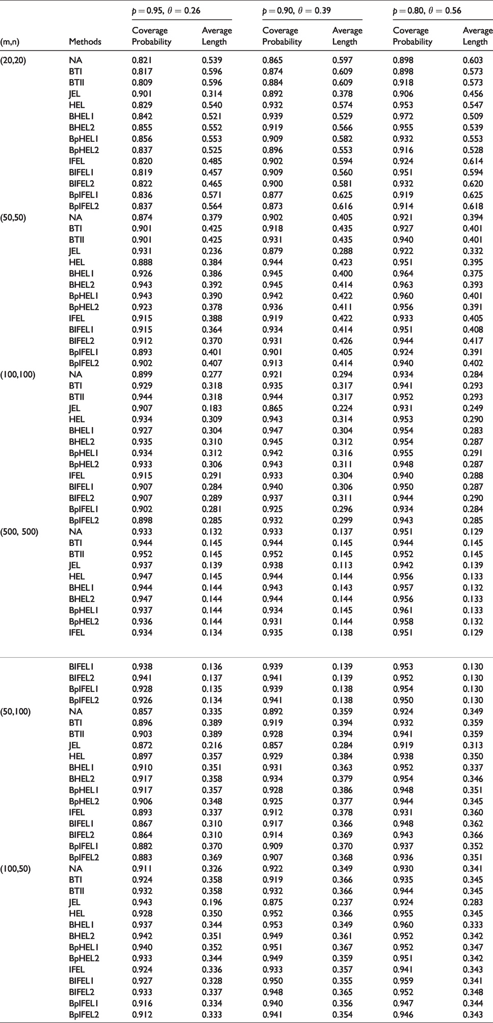
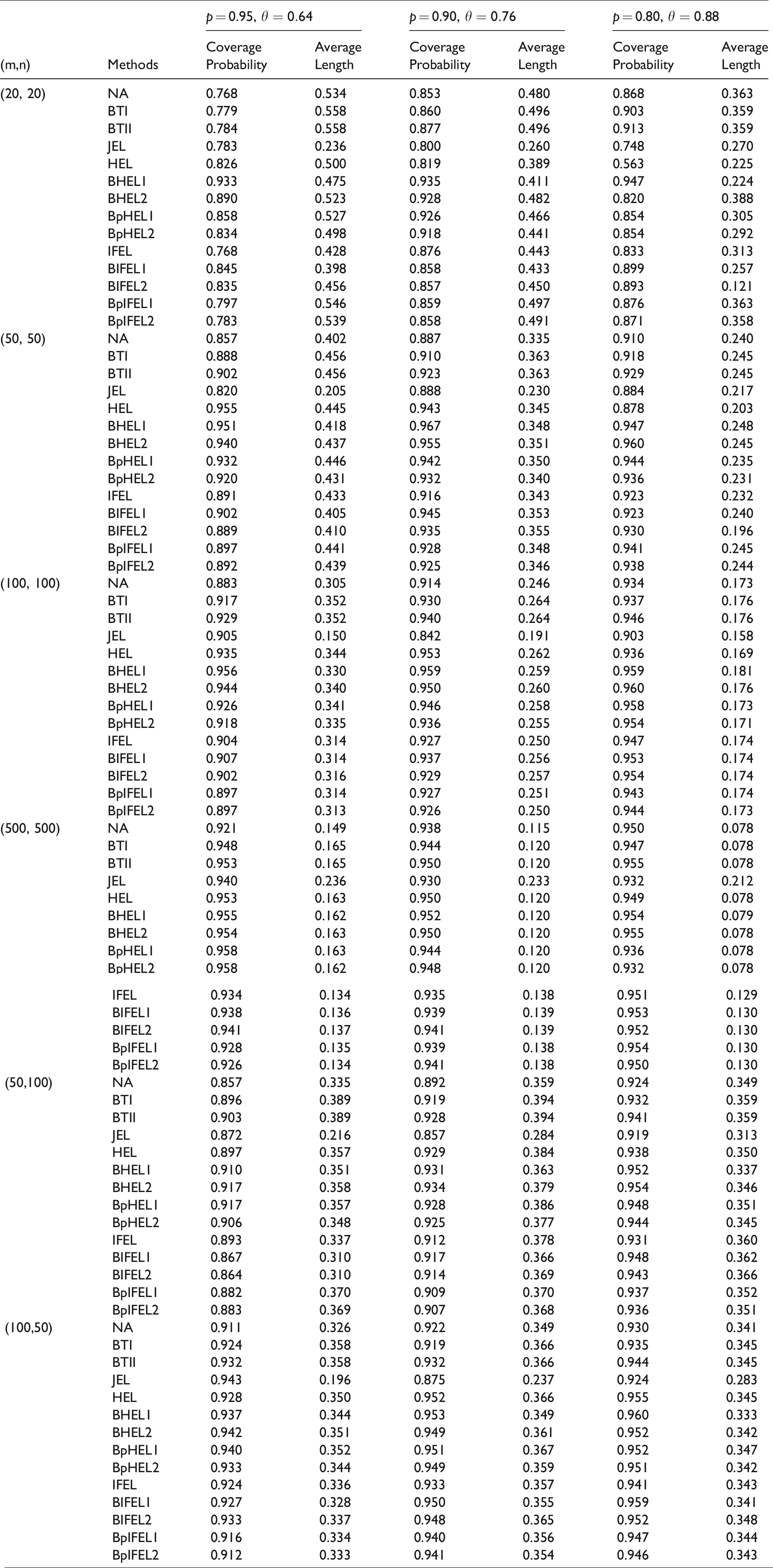
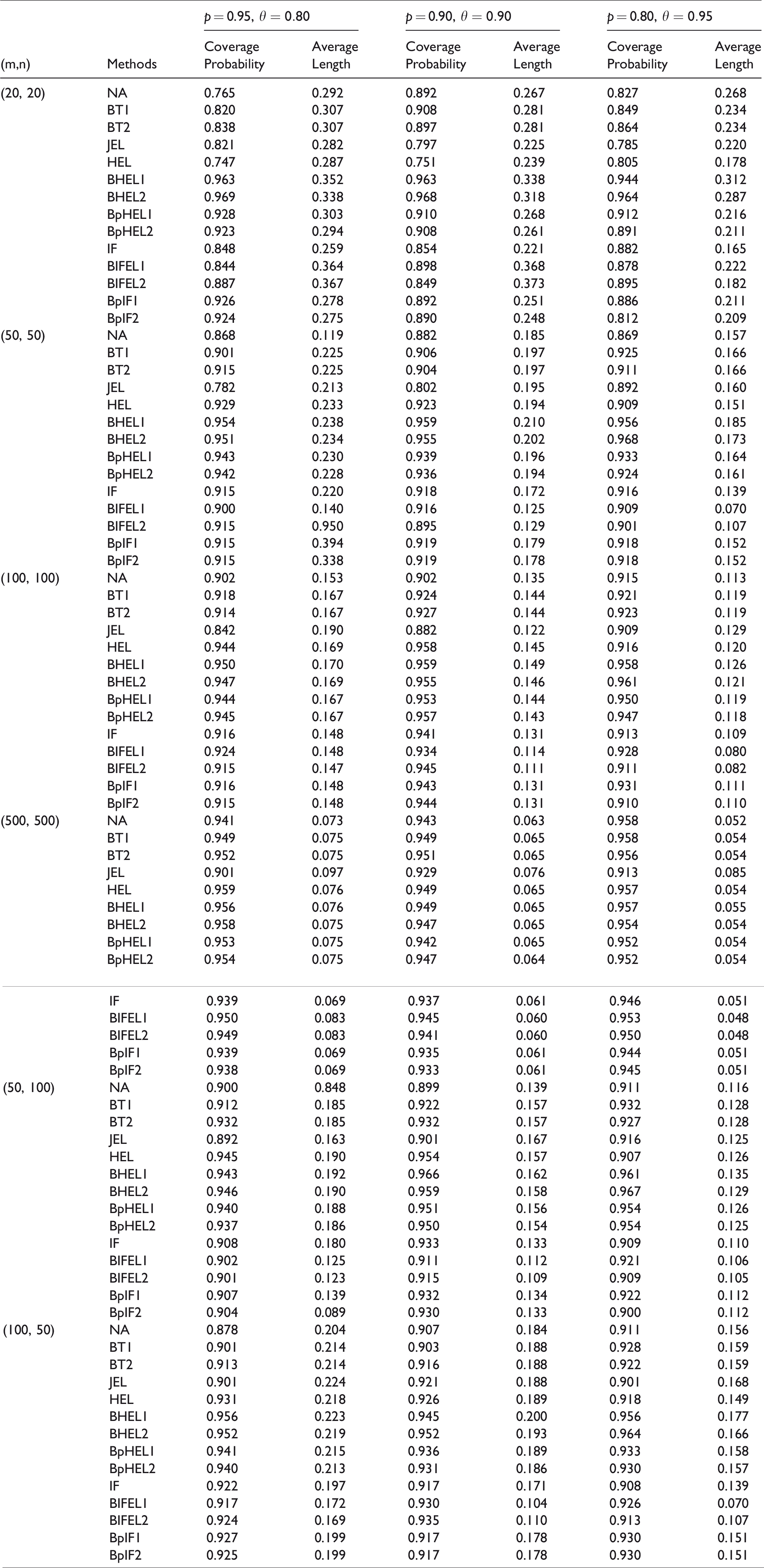
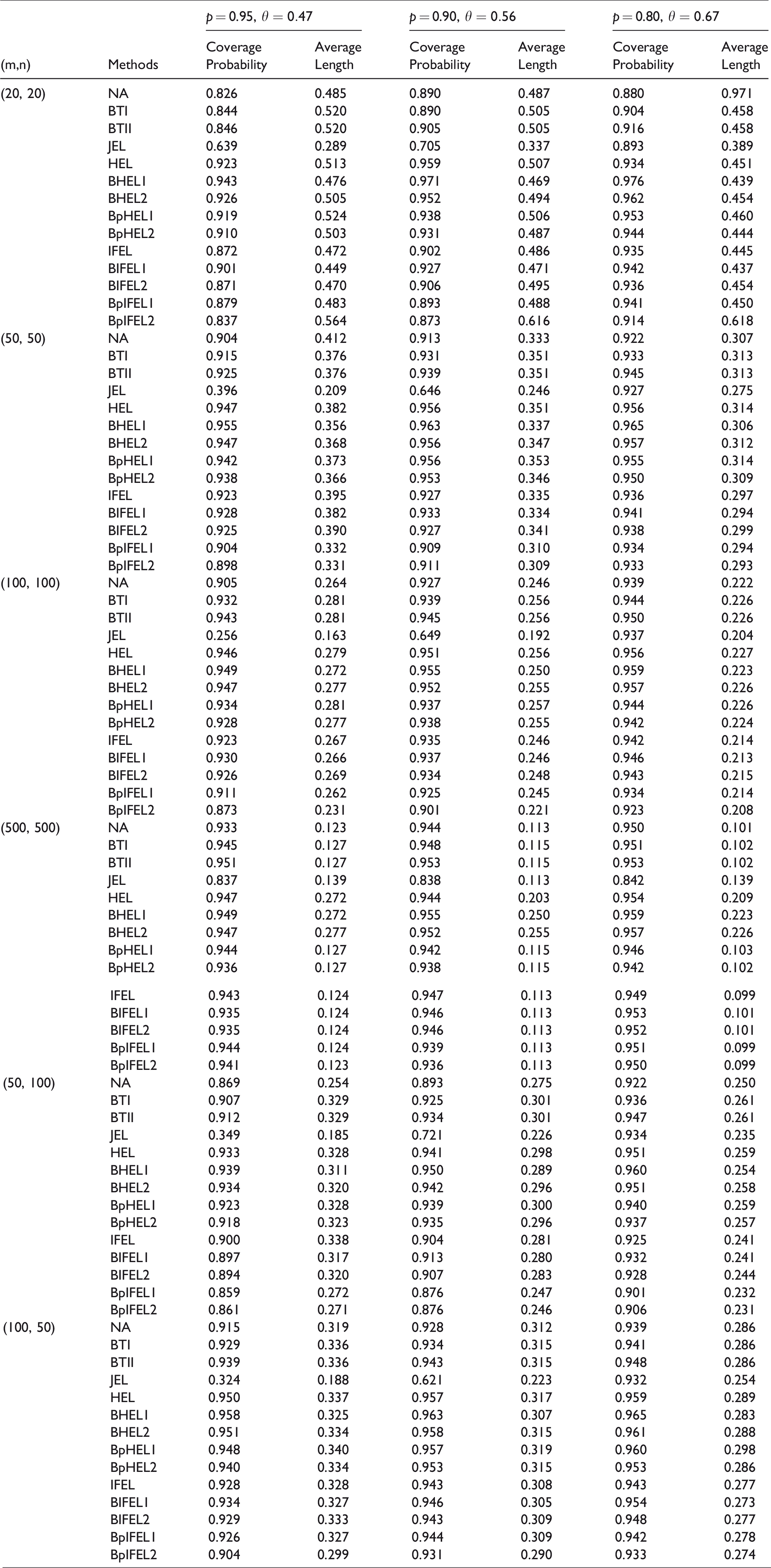
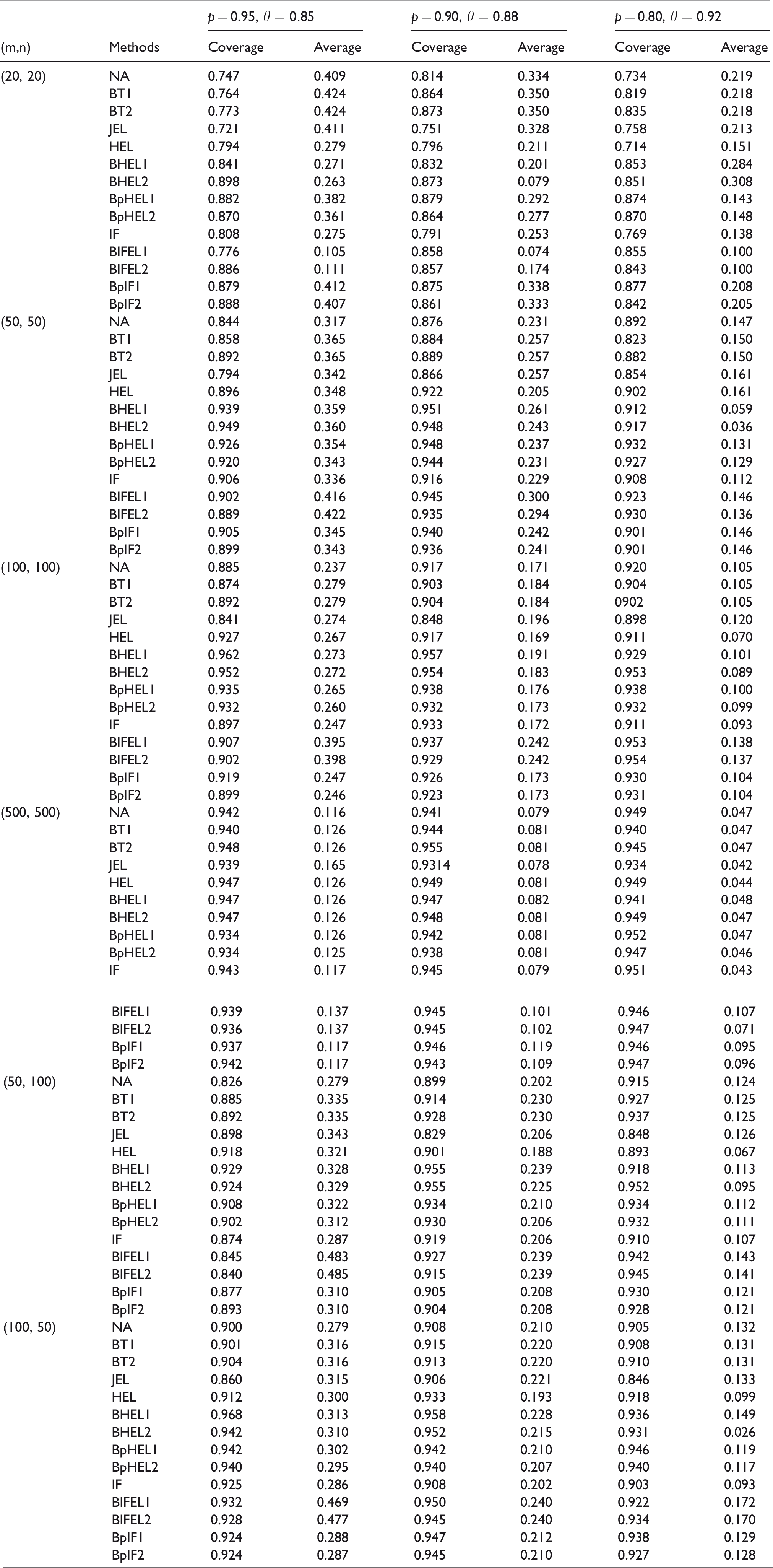
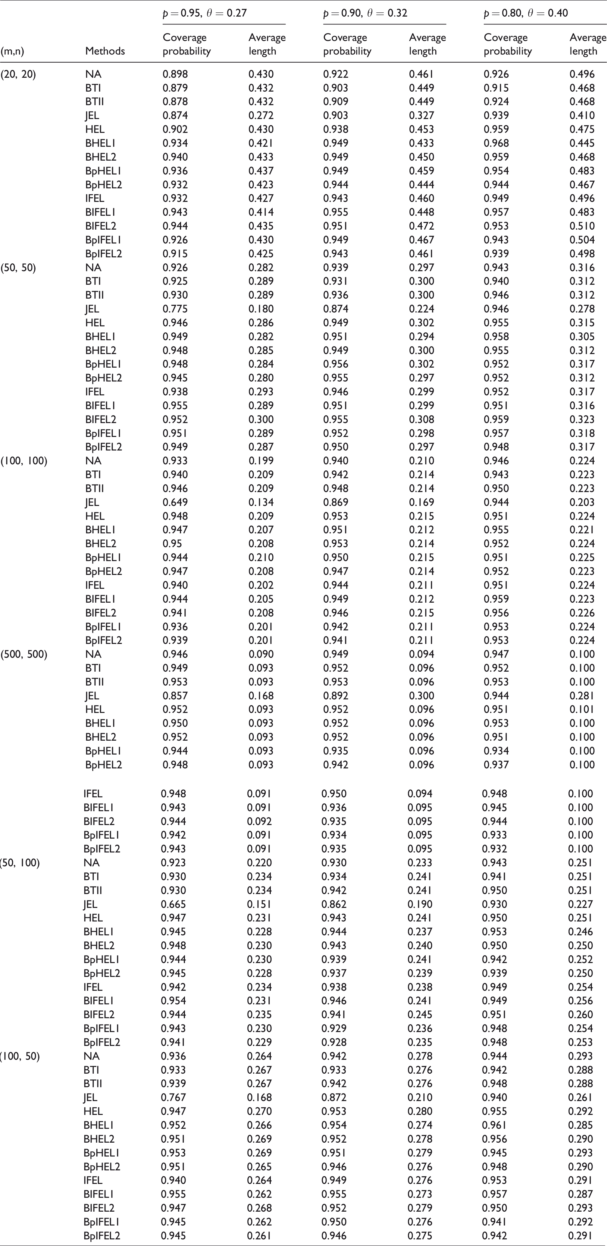
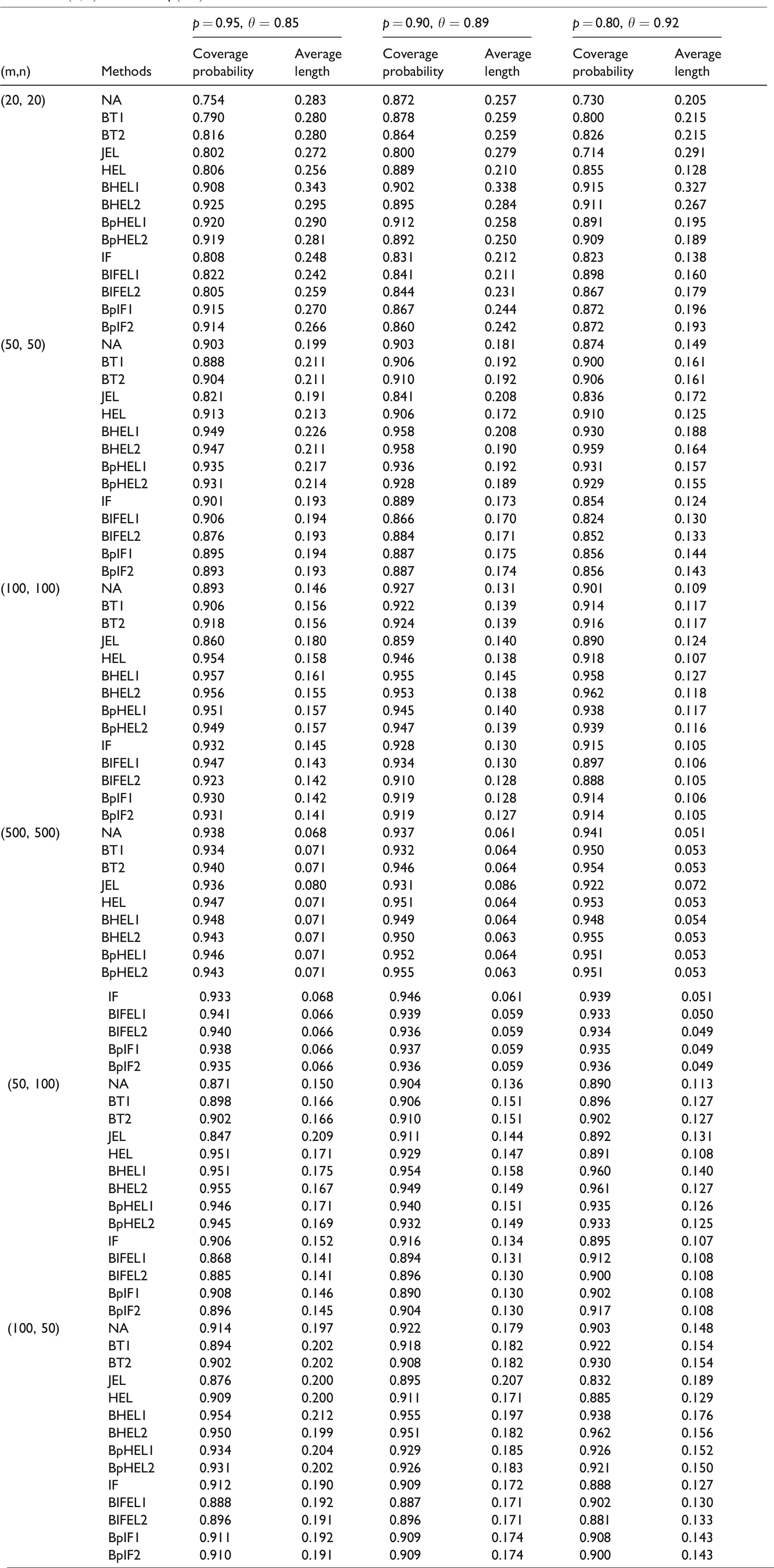

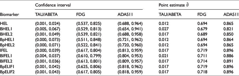
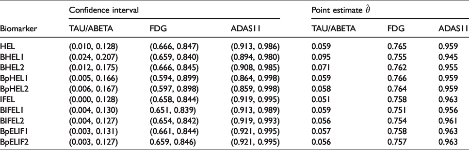
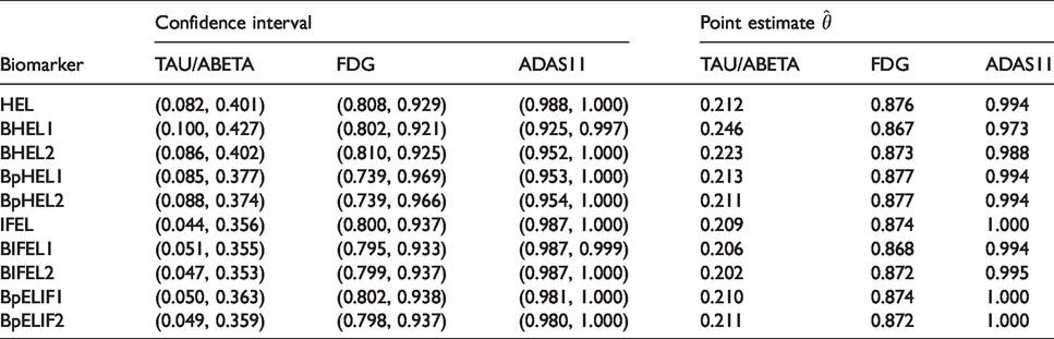
 ). The grantee organization is the Northern California Institute for Research and Education, and the study is coordinated by the Alzheimer’s Therapeutic Research Institute at the University of Southern California. ADNI data are disseminated by the Laboratory for Neuro Imaging at the University of Southern California.