Influence function-based empirical likelihood for area under the receiver operating characteristic curve in presence of covariates

Abstract

In receiver operating characteristicROC analysis, the area under the ROC curve (AUC) is a popular one number summary of the discriminatory accuracy of a diagnostic test. AUC measures the overall diagnostic accuracy of a test but fails to account for the effect of covariates when covariates are present and associated with the test results. Adjustment for covariate effects can greatly improve the diagnostic accuracy of a test. In this paper, using information provided by the influence function, empirical likelihood (EL) methods are proposed for inferences of AUC in presence of covariates. For parameters in the AUC regression model, it is shown that the asymptotic distribution of the influence function-based empirical log-likelihood ratio statistic is a standard chi-square distribution. Hence, confidence regions for the regression parameters can be obtained without any variance estimation. Simulation studies are conducted to compare the finite sample performances of the proposed EL based methods with the existing normal approximation (NA) based method in the AUC regression. Simulation results indicate that the bootstrap-calibrated influence function-based empirical likelihood (BIFEL ) confidence region outperforms the NA-based confidence region in terms of coverage probability. We also propose an interval estimation method for the covariate-adjusted AUC based on the BIFEL confidence region. Finally, we illustrate the recommended method with a real prostate-specific antigen data example.

Keywords

Bootstrap confidence region covariate-adjusted area under the receiver operating characteristic curve empirical likelihood influence function

1. Introduction

In medical diagnostic studies, the receiver operating characteristic (ROC) curve of a medical test is the plot of sensitivity versus one minus specificity of the test across all possible cut-off values.¹ The area under the ROC curve (AUC) is a popular summary index for the diagnostic accuracy of the test. While AUC measures overall diagnostic accuracy of a test but fails to account for the effect of covariates when some covariates/factors are present and associated with the test results. It is well known that the value of AUC for a test can vary across different population subgroups, test types, settings, and depending on the position of the test in the clinical pathway.^2,3 For example, male patients often exhibit higher hemoglobin levels compared to female patient; African American men tend to have higher prostate-specific antigen (PSA, a prostate cancer biomarker) levels relative to men from other racial backgrounds^4,5; and PSA can be higher in older men.⁶ In presence of covariates, there may be covariate-specific (such as age, gender and race) differences in test performance. Moreover, when strong associations between the test results and covariates are present, choosing a cut-off from a ROC curve without covariate-adjustment can be misleading, compared to using covariate-specific ROC curves. Lee et al.⁷ presented a motivating example and an application of methods that incorporate covariates in ROC curve analysis, using individual patient data on D-dimer testing for excluding pulmonary embolism. Consequently, when covariate information is available, covariate-adjusted ROC analysis (e.g., covariate-adjusted sensitivity, specificity, ROC curve, AUC, Yuden index, etc) is essential for evaluating the diagnostic accuracy of a medical test.

Covariate-adjustments for summary measures of the ROC curve have become critical in many diagnostic contexts. Since the operating conditions of the test or patients characteristics such as gender, age, race, physical conditions and so on, may affect the test results by influencing the distributions of test measurements for “diseased” and/or “non-diseased” subjects, extensive research has focused on incorporating covariates information into ROC analysis. For example, Thompson and Zucchini⁸ and Obuchowski⁹ proposed AUC regression methods based on the derived variables; Dorfman, Berbaum, and Metz¹⁰ developed a method involving jackknife AUC values for each subject. Dodd and Pepe^11,12 proposed a regression model for AUC, while Liu and Zhou¹³ provided covariate adjustment in estimating the AUC with partially missing gold standard. Meng and Tubbs¹⁴ applied a beta regression model for covariate adjusted ROC analysis.

Empirical likelihood (EL)^15,16 is a powerful non-parametric method and its advantages over the normal approximation (NA)-based methods have been well-recognized.¹⁷ For instance, the EL-based approach allows the construction of confidence intervals/regions without requiring a variance estimator; instead of assuming a symmetric shape for these confidence intervals/regions, EL derives the shape directly from the data. EL has been widely used in various fields. Readers are referred to Owen’s¹⁸ book and references therein. EL-based techniques have also been successfully applied to ROC analysis.^19,20 In this paper, we introduce a novel combination of EL, influence functions, and covariates for inference on AUC through the AUC regression model. Our proposed bootstrap-calibrated influence function-based empirical likelihood (BIFEL ) method outperforms the existing normal approximation (NA) based method in the AUC regression in terms of coverage probability. We also propose an interval estimation method for the covariate-adjusted AUC based on the BIFEL confidence region.

This paper is organized as follows. In Section 2, we review a direct modeling and inference method for AUC in the presence of covariates. In Section 3, we propose an Influence Function-based EL (IFEL) method and a Jackknife-EL (JEL) method for constructing confidence regions of the regression parameter vector in AUC regression model when covariates information is available. In Section 4, we conduct simulation studies to compare the proposed EL-based methods with the existing NA-based method. In Sections 5, we propose a BIFEL-based confidence interval for the covariate-adjusted AUC. In Section 6, we apply the recommended method to a real PSA dataset. Finally, the proof of the main theorem is presented in Appendix.

2. Direct modeling and inference for AUC in presence of covariates

Dodd and Pepe¹¹ proposed a direct modeling and inference method on AUC in presence of covariates. Let ${(Y_{i}^{\bar{D}}, Z_{i}^{\bar{D}}) : i = 1, \dots, m}$ be a sample from the population $(Y^{\bar{D}}, Z^{\bar{D}})$ of non-diseased subjects with test result $Y_{i}^{\bar{D}}$ and covariates $Z_{i}^{\bar{D}}$ , and ${(Y_{j}^{D}, Z_{j}^{D}) : j = 1, \dots, n}$ be a sample from the population $(Y^{D}, Z^{D})$ of diseased subjects with test result $Y_{j}^{D}$ and covariates $Z_{j}^{D}$ . Let $θ_{i j} = P (Y_{j}^{D} > Y_{i}^{\bar{D}} | Z_{i}^{\bar{D}}, Z_{j}^{D})$ be the covariate-specific AUC parameter. Dodd and Pepe¹¹ directly model the AUC in presence of covariates as follows:

θ_{i j} = g (β^{T} Z_{i j})

(1)

where

Z_{i j}

denotes the observable covariates

(Z_{i}^{\bar{D}}, Z_{j}^{D})

g

is a specified function,

β

is a

p

-dimensional regression vector of interest.

For estimating $β$ , the following estimation equation can be used (see Dodd and Pepe¹¹)

\sum_{j = 1}^{n} \sum_{i = 1}^{m} \frac{\partial θ_{i j}}{\partial β} ω (Z_{i j}, β) (I_{i j} - g (β^{T} Z_{i j})) = 0

(2)

where

I_{i j} = I (Y_{j}^{D} > Y_{i}^{\bar{D}})

, and

ω (Z_{i j}, β)

is a known weight function

Let $\hat{β}$ be the estimator for $β$ based on the above estimation equation. Dodd and Pepe¹¹ showed that the distribution of $\hat{β}$ is asymptotically normal, i.e.,

\sqrt{\frac{m n}{m + n}} (\hat{β} - β) \overset{L}{⟶} N (0, Ξ), as m + n \to \infty

(3)

where

Ξ

is the asymptotic variance of

\hat{β}

Using (3), a $(1 - α)$ ( $0 < α < 1$ ) level NA-based confidence region for $β$ can be constructed as follows:

C R_{N A} (β) = {β : \frac{m + n}{m n} \cdot (\hat{β} - β)^{T} {\hat{Ξ}}^{- 1} (\hat{β} - β) \leq χ_{p, 1 - α}^{2}}

(4)

where

\hat{Ξ}

is an estimate for the asymptotic variance of

\hat{β}

, and

χ_{p, 1 - α}^{2}

is the

(1 - α)

th quantile of

χ_{p}^{2}

distribution.

This NA-based confidence region for $β$ can be used to make inference for $β$ if there is a good estimate for the asymptotic variance matrix $Ξ$ . Although $\hat{Ξ}$ can be obtained based on estimation methods with generalized linear models (GLMs) (e.g., using vcov function in R), the NA-based confidence region for $β$ can have poor coverage accuracy (see our simulation results in Section 4). To avoid the variance estimation, in next section, we propose a new IFEL for AUC in presence of covariates.

3. EL-based confidence regions of

β

in the covariate adjusted AUC regression model

3.1. Confidence region of $β$ based on IFEL method

Let $Y$ be the continuous-scale test result which can be used for discrimination between the “diseased” and “non-diseased” groups. $Y$ can be standardized according to the distribution $F_{Z^{\bar{D}}}^{\bar{D}}$ (called the reference distribution²¹) in the non-diseased population. The placement value of $Y$ is defined as $U = 1 - F_{Z^{\bar{D}}}^{\bar{D}} (Y)$ . In particular, $U^{\bar{D}} = 1 - F_{Z^{\bar{D}}}^{\bar{D}} (Y^{\bar{D}})$ is uniform on $(0, 1)$ , and $U^{D} = 1 - F_{Z^{\bar{D}}}^{\bar{D}} (Y^{D})$ measures the separation between the diseased and non-diseased groups. The ROC curve and the placement value have a closed relationship. If setting $u = 1 - F_{Z^{\bar{D}}}^{\bar{D}} (y)$ as a false positive rate, then the conditional distribution of $U^{D}$ given $Z^{D}$ is the conditional ROC curve, i.e., $R O C_{Z} (u) = P (U^{D} < u | Z^{D}) .$ The covariate-adjusted AUC can be expressed as $A U C_{Z} = E (1 - U^{D} | Z^{D}) .$ The covariate effects on discrimination of a test can be evaluated by using the following AUC regression model^11,21:

A U C_{Z} = E (1 - U^{D} | Z^{D}) = g (β^{T} Z^{D})

(5)

where

β

is a

p

-dimensional unknown regression coefficient,

Z^{D} = (Z_{1}^{D}, \dots, Z_{p}^{D})^{T}

is the

p \times 1

vector of covariates,

g

is a specified link function.

To estimate $β$ , we use the following GLM re-weighted least squares fitting-based estimation equation:

\sum_{j = 1}^{n} [1 - U_{j}^{D} - g (β^{T} Z_{j}^{D})] ω (β^{T} Z_{j}^{D}) Z_{j}^{D} \equiv \sum_{j = 1}^{n} H_{j} = 0

(6)

where

ω (β^{T} Z_{j}^{D})

is a given scalar weight function,

0 = (0, \dots, 0)^{T}

is a

p \times 1

vector,

Z_{j}^{D}

is the

p \times 1

vector of covariates for the

j

th diseased subject, and

H_{j} = (1 - U_{j}^{D} - g (β^{T} Z_{j}^{D})) ω (β^{T} Z_{j}^{D}) Z_{j}^{D}

(7)

Since the distribution function $F_{Z^{\bar{D}}}^{\bar{D}}$ is unknown, the placement value $U^{D} = 1 - F_{Z^{\bar{D}}}^{\bar{D}} (Y^{D})$ is unobservable. However, with the non-diseased sample ${(Y_{i}^{\bar{D}}, Z_{i}^{\bar{D}}), i = 1, 2, \dots, m}$ , we can estimate $F_{Z^{\bar{D}}}^{\bar{D}}$ by its empirical distribution ${\hat{F}}_{Z^{\bar{D}}}^{\bar{D}}$ . Hence, the placement value $U_{j}^{D} = 1 - F_{Z^{\bar{D}}}^{\bar{D}} (Y_{j}^{D})$ can be estimated by ${\hat{U}}_{j}^{D} = 1 - {\hat{F}}_{Z^{\bar{D}}}^{\bar{D}} (Y_{j}^{D})$ , and $\hat{β}$ , an estimator for $β$ , can be obtained by solving the following estimation equation:

\sum_{j = 1}^{n} [1 - {\hat{U}}_{j}^{D} - g (β^{T} Z_{j}^{D})] ω (β^{T} Z_{j}^{D}) Z_{j}^{D} \equiv \sum_{j = 1}^{n} {\hat{H}}_{j} = 0

(8)

where

{\hat{H}}_{j} = (1 - {\hat{U}}_{j}^{D} - g (β^{T} Z_{j}^{D})) ω (β^{T} Z_{j}^{D}) Z_{j}^{D}

(9)

Let ${(Y_{k}, Z_{k}), k = 1, \dots, n + m} = {(Y_{1}^{D}, Z_{1}^{D}), \dots, (Y_{n}^{D}, Z_{n}^{D})$ , $(Y_{1}^{\bar{D}}, Z_{1}^{\bar{D}}), \dots, (Y_{m}^{\bar{D}}, Z_{m}^{\bar{D}})}$ . From (7) and (9) (see also the proof of Lemma 1 in Appendix), it follows that

\begin{aligned} \frac{1}{\sqrt{n + m}} \sum_{j = 1}^{n} {\hat{H}}_{j} & = \frac{1}{\sqrt{n + m}} \sum_{j = 1}^{n} H_{j} + \frac{n}{m} [lim_{n \to \infty} \frac{1}{n} \sum_{j = 1}^{n} ω (β^{T} Z_{j}^{D}) Z_{j}^{D}] \\ \times \frac{1}{\sqrt{n + m}} \sum_{i = 1}^{m} (\int I (Y_{i}^{\bar{D}} \leq t) d F_{Z^{D}}^{D} (t) - \int F_{Z^{\bar{D}}}^{\bar{D}} (t) d F_{Z^{D}}^{D} (t)) + o_{p} (1) \\ = \frac{1}{\sqrt{n + m}} \sum_{j = 1}^{n} H_{j} + \frac{ρ A (β)}{\sqrt{n + m}} \sum_{i = 1}^{m} \int (I (Y_{i}^{\bar{D}} \leq t) - F_{Z^{\bar{D}}}^{\bar{D}} (t)) d F_{Z^{D}}^{D} (t) + o_{p} (1) \\ \equiv \frac{1}{\sqrt{n + m}} \sum_{k = 1}^{n + m} W_{k} (β) + o_{p} (1) \end{aligned}

where

ρ = lim_{n \to \infty} \frac{n}{m}

A (β) = lim_{n \to \infty} \frac{1}{n} \sum_{j = 1}^{n} ω (β^{T} Z_{j}^{D}) Z_{j}^{D}

, and

\begin{aligned} W_{k} (β) = {\begin{array}{cccc} H_{k}, & if k = 1, \dots, n, \\ ρ A (β) \int (I (Y_{k} \leq t) - F_{Z^{\bar{D}}}^{\bar{D}} (t)) d F_{Z^{D}}^{D} (t), & if k = n + 1, \dots, n + m \end{array} \end{aligned}

is called the

k

th influence function of

\hat{β}

k = 1, \dots, n + m

Using the information provided by the influence function, the EL for $β$ can be defined as follows:

L_{I F} (β) = sup {\prod_{k = 1}^{n + m} p_{k} : p_{1} \geq 0, \dots, p_{n + m} \geq 0, \sum_{j = 1}^{n + m} p_{k} = 1, \sum_{k = 1}^{n + m} p_{k} {\hat{W}}_{k} (β) = 0}

(10)

where

\begin{aligned} {\hat{W}}_{k} (β) = {\begin{array}{cccc} {\hat{H}}_{k}, & if k = 1, \dots, n, \\ \frac{1}{m} \sum_{j = 1}^{n} ω (β^{T} Z_{j}^{D}) Z_{j}^{D} \int (I (Y_{k} \leq t) - {\hat{F}}_{Z^{\bar{D}}}^{\bar{D}} (t)) d {\hat{F}}_{Z^{D}}^{D} (t), & if k = n + 1, \dots, n + m \end{array} \end{aligned}

is the

k

th estimated influence function,

{\hat{F}}_{Z^{\bar{D}}}^{\bar{D}} (t) = \frac{1}{m} \sum_{i = 1}^{m} I (Y_{i}^{\bar{D}} \leq t)

, and

{\hat{F}}_{Z^{D}}^{D} (t) = \frac{1}{n} \sum_{j = 1}^{n} I (Y_{j}^{D} \leq t)

Using the Lagrange multiplier method, we get that

p_{k} = \frac{1}{n + m} \frac{1}{1 + ν^{T} {\hat{W}}_{k} (β)},

where

ν^{T} = (ν_{1}, ν_{2}, \dots, ν_{p})

is the solution to

\frac{1}{n + m} \sum_{k = 1}^{n + m} \frac{{\hat{W}}_{k} (β)}{1 + ν^{T} {\hat{W}}_{k} (β)} = 0

(11)

Note that

\prod_{k = 1}^{n + m} p_{k}

, subject to

\sum_{k = 1}^{n + m} p_{k} = 1, p_{k} \geq 0, k = 1, 2, \dots, n + m

, attains its maximum

(n + m)^{- (n + m)}

p_{k} = (n + m)^{- 1}

. So, the influence function-based EL ratio for

β

R_{I F} (β) = \prod_{k = 1}^{n + m} (n + m) p_{k} = \prod_{k = 1}^{n + m} {1 + ν^{T} {\hat{W}}_{k} (β)}^{- 1}

The corresponding influence function-based empirical log-likelihood ratio for

β

l_{I F} (β) = - 2 \log R_{I F} (β) = 2 \sum_{k = 1}^{n + m} \log {1 + ν^{T} {\hat{W}}_{k} (β)}

Theorem 1

If $max_{j} ‖ Z_{j}^{D} ‖ = o_{p} (n^{1 / 2})$ , $lim_{n, m \to \infty} \frac{n}{m} = ρ > 0$ , $g$ and $ω$ are bounded functions, and $β$ is the regression parameter vector in the AUC regression model (5), then the asymptotic distribution of the influence function-based empirical log-likelihood ratio statistic $l_{I F} (β)$ is a chi-square distribution with $p$ degree of freedom. That is,

l_{I F} (β) \overset{L}{⟶} χ_{p}^{2}

(12)

The proof of Theorem 1 is provided in the Appendix. Using Theorem 1, a $(1 - α)$ level IFEL-based confidence region for $β$ can be constructed as follows:

C R_{I F} (β) = {β : l_{I F} (β) \leq χ_{p, 1 - α}^{2}}

where

χ_{p, 1 - α}^{2}

is the

(1 - α)

th quantile of

χ_{p}^{2}

3.2. Confidence region of

β

based on JEL method

JEL, proposed by Jing, Yuan, and Zhou,²² is another powerful non-parametric method to overcome the computational difficulties dealing with nonlinear functionals. Using the techniques in Jing, Yuan and Zhou,²² we can define the JEL for $β$ . Let

\begin{aligned} T_{n + m} (β) = & \frac{1}{n + m} \sum_{k = 1}^{n + m} {\hat{W}}_{k} (β), \\ T_{n + m, - i} (β) = & \frac{1}{n + m - 1} \sum_{k = 1, k \neq i}^{n + m} {\hat{W}}_{k, - i} (β), i = 1, 2, \dots, n + m \end{aligned}

where

{\hat{W}}_{k, - i} (β)

is the

{\hat{W}}_{k} (β)

based on the

n + m - 1

observations from

{(Y_{k}, Z_{k}), k = 1, \dots, n + m}

by deleting the

i

th observation

(Y_{i}, Z_{i})

Then the jackknife pseudo sample can be written as:

{\tilde{W}}_{i} (β) = (n + m) T_{n + m} (β) - (n + m - 1) T_{n + m, - i} (β), i = 1, 2, \dots, n + m

Applying Owen’s EL to this jackknife pseudo sample, we get the following JEL for

β

L_{J} (β) = sup {\prod_{k = 1}^{n + m} p_{k} : p_{1} \geq 0, \dots, p_{n + m} \geq 0, \sum_{j = 1}^{n + m} p_{k} = 1, \sum_{k = 1}^{n + m} p_{k} {\tilde{W}}_{k} (β) = 0}

(13)

The corresponding jackknife empirical log-likelihood ratio for

β

l_{J} (β) = 2 \sum_{k = 1}^{n + m} \log (1 + ν_{J}^{T} {\tilde{W}}_{k} (β))

where

ν_{J}^{T} = (ν_{J 1}, ν_{J 2}, \dots, ν_{J p})

is the solution to

\frac{1}{n + m} \sum_{k = 1}^{n + m} \frac{{\tilde{W}}_{k} (β)}{1 + ν_{J}^{T} {\tilde{W}}_{k} (β)} = 0

(14)

Under the same conditions as in Theorem 1, we assume that the asymptotic distribution of the empirical log-likelihood ratio statistic $l_{J} (β)$ is a standard chi-square distributions with $p$ degree of freedom. That is,

l_{J} (β) \overset{L}{⟶} χ_{p}^{2}

(15)

Then, a

(1 - α)

level JEL-based confidence region (JEL region) for

β

can be constructed as

C R_{J} (β) = {β : l_{J} (β) \leq χ_{p, 1 - α}^{2}}

(16)

4. Simulation studies

In this section, we conduct simulation studies to evaluate finite sample performances of the proposed IFEL-based confidence region and the JEL-based confidence region in presence of covariates. Particularly, we compare the IFEL and JEL confidence regions with the existing NA-based confidence region for $β$ in the AUC regression model (5) in terms of coverage probability. Two simulation scenarios are considered in these studies.

Scenario 1: The link function $g$ for $A U C_{Z}$ is the standard normal distribution $Φ (\cdot)$ (a simulation setting like that used in Dodd and Pepe¹¹).

Under this scenario, we generate data from linear models $Y^{D} = k^{T} Z^{D} + e_{1}$ with $e_{1} \sim N (0, σ_{D}^{2})$ , and $Y^{\bar{D}} = γ^{T} Z^{\bar{D}} + e_{2}$ with $e_{2} \sim N (0, σ_{\bar{D}}^{2})$ . Then, we have that $A U C_{Z} = Φ (β^{T} Z)$ .

Case I (The dimension of $β$ is $p = 2$ ): Our simulated data are generated from the linear models $Y_{j}^{D} = k_{0} + k_{1} Z_{j}^{D} + e_{1, j}$ with $e_{1, j} \sim N (0, σ_{D}^{2})$ , and $Y_{i}^{\bar{D}} = γ_{0} + γ_{1} Z_{i}^{\bar{D}} + e_{2, i}$ with $e_{2, i} \sim N (0, σ_{\bar{D}}^{2})$ , where the covariates $Z_{j}^{D}$ ’s and $Z_{i}^{\bar{D}}$ ’s are assumed to follow the uniform distribution $Z \sim U (0, 10)$ , $k_{0} = 0$ , $k_{1} = 0.5$ , $σ_{D} = 1.2$ , $γ_{0} = 0$ , $γ_{1} = 0$ , and $σ_{\bar{D}} = 1$ . Then the AUC regression model is

A U C_{Z} = Φ (\frac{(k_{0} - γ_{0}) + (k_{1} - γ_{1}) Z}{\sqrt{σ_{D}^{2} + σ_{\bar{D}}^{2}}}) = Φ (β_{0} + β_{1} Z)

(17)

with true parameters

β_{0} = (k_{0} - γ_{0}) / \sqrt{σ_{D}^{2} + σ_{\bar{D}}^{2}} = 0,

and

β_{1} = (k_{1} - γ_{1}) / \sqrt{σ_{D}^{2} + σ_{\bar{D}}^{2}} = 0.32.

Case II (The dimension of $β$ is $p = 3$ ): Our simulated data are generated from the linear models $Y_{j}^{D} = k_{0} + k_{1} Z_{1, j}^{D} + k_{2} Z_{2, j}^{D} + e_{1, j}$ with $e_{1, j} \sim N (0, σ_{D}^{2})$ , and $Y_{i}^{\bar{D}} = γ_{0} + γ_{1} Z_{1, i}^{\bar{D}} + γ_{2} Z_{2, i}^{\bar{D}} + e_{2, i}$ with $e_{2, i} \sim N (0, σ_{\bar{D}}^{2})$ , where the covariates $Z_{1, j}^{D}$ ’s and $Z_{1, i}^{\bar{D}}$ ’s are assumed to follow $Z_{1} \sim U (0, 10)$ , and the covariates $Z_{2, j}^{D}$ ’s and $Z_{2, i}^{\bar{D}}$ ’s are assumed to follow $Z_{2} \sim N (1.2, 3)$ , respectively, $k_{0} = 1$ , $k_{1} = 0.8,$ $k_{2} = 1.7$ , $σ_{D} = 1.2$ , $γ_{0} = 0.7,$ $γ_{1} = 0.5,$ $γ_{2} = 0.3$ , and $σ_{\bar{D}} = 1$ . Then the AUC regression model is

A U C_{Z} = Φ (β_{0} + β_{1} Z_{1} + β_{2} Z_{2})

(18)

with true parameter values

β_{0} = 0.192,

β_{1} = 0.192,

and

β_{2} = 0.896

Since the standard $χ_{p}^{2}$ approximation to the distribution of the empirical log-likelihood ratio statistic $l_{I F} (β)$ in Theorem 1 may not be good enough for confidence region estimation of $β$ with finite sample sizes, we propose the following bootstrap calibration procedure to construct a confidence region for $β$ .

Generate samples from $Y_{j}^{D} = k^{T} {Z_{j}}^{D} + e_{1, j}$ with $e_{1, j}$ generated from $N (0, σ_{D}^{2})$ , and $Y_{i}^{\bar{D}} = γ^{T} {Z_{i}}^{\bar{D}} + e_{2, i}$ with $e_{2, i}$ generated from $N (0, σ_{\bar{D}}^{2})$ , where ${Z_{j}}^{D}$ ’s and ${Z_{i}}^{\bar{D}}$ ’s are generated according to the distributions described in Case I or Case II, respectively.

Draw a bootstrap resample $e_{1, j}^{*}$ ’s from the residuals $e_{1, j}$ ’s for the “diseased” group to get the bootstrap version $({Z_{j}}^{D}, Y_{j}^{D, *})$ ’s of $({Z_{j}}^{D}, Y_{j}^{D})$ ’s, and draw a bootstrap resample $e_{2, i}^{*}$ ’s from the residuals $e_{2, i}$ ’s for the “non-diseased” group to get the bootstrap version $({Z_{i}}^{\bar{D}}, Y_{i}^{\bar{D}, *})$ ’s of $({Z_{i}}^{\bar{D}}, Y_{i}^{\bar{D}})$ ’s.

Apply the estimation method for the GLM to get the estimate ${\hat{β}}^{*}$ for $β$ and compute a bootstrap copy $l_{I F}^{*} ({\hat{β}}^{*})$ of $l_{I F} (\hat{β})$ based on the bootstrap resamples $({Z_{j}}^{D}, Y_{j}^{D, *})$ ’s and $({Z_{i}}^{\bar{D}}, Y_{i}^{\bar{D}, *})$ ’s.

Repeat steps 2-3 $B$ ( $B \geq 200$ is recommended) times to obtain $B$ bootstrap copies ${l_{I F}^{* b} ({\hat{β}}^{*}), b = 1, \dots, B}$ of $l_{I F} (\hat{β})$ .

Then a $(1 - α)$ level bootstrap-calibrated IFEL (called BIFEL) confidence region for $β$ can be constructed as follows:

C R_{B I F} (β) = {β : l_{I F} (β) \leq χ_{(1 - α)}}

where

χ_{(1 - α)}

is the

(1 - α)

th quantile of

{l_{I F}^{* b} ({\hat{β}}^{*}), b = 1, \dots, B}

Similarly, we can apply bootstrap calibration to the jackknife empirical log-likelihood ratio statistic $l_{J} (β)$ to get a $(1 - α)$ level bootstrap-calibrated JEL (called BJEL) confidence region for $β$ . In our simulation studies, we compare the IFEL confidence region, the JEL confidence region, with the BIFEL and BJEL confidence regions for $β$ in the AUC regression model in terms of coverage probability.

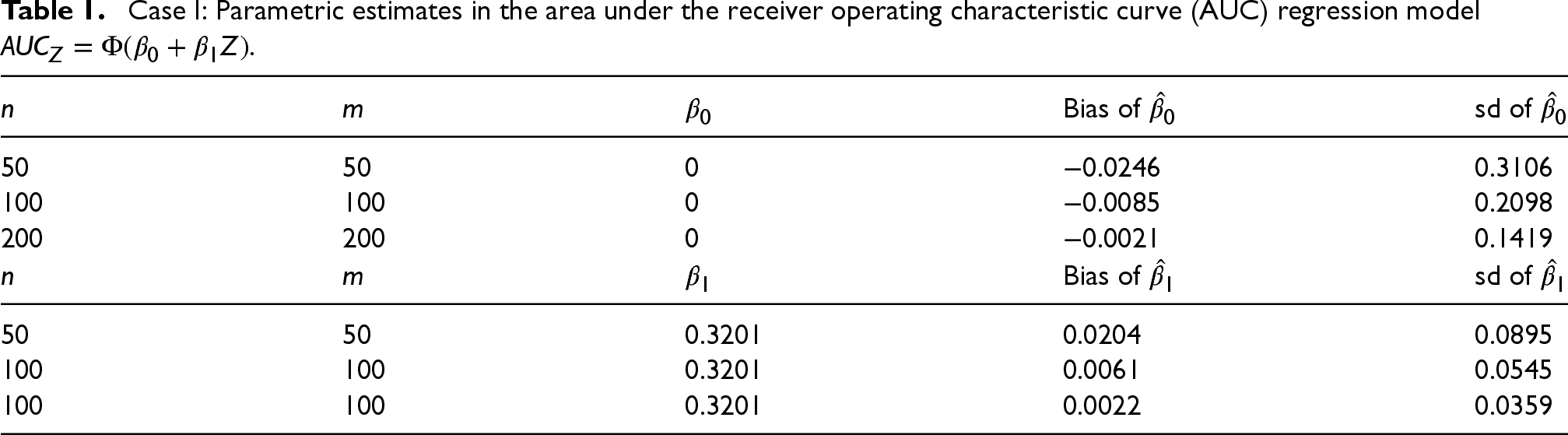
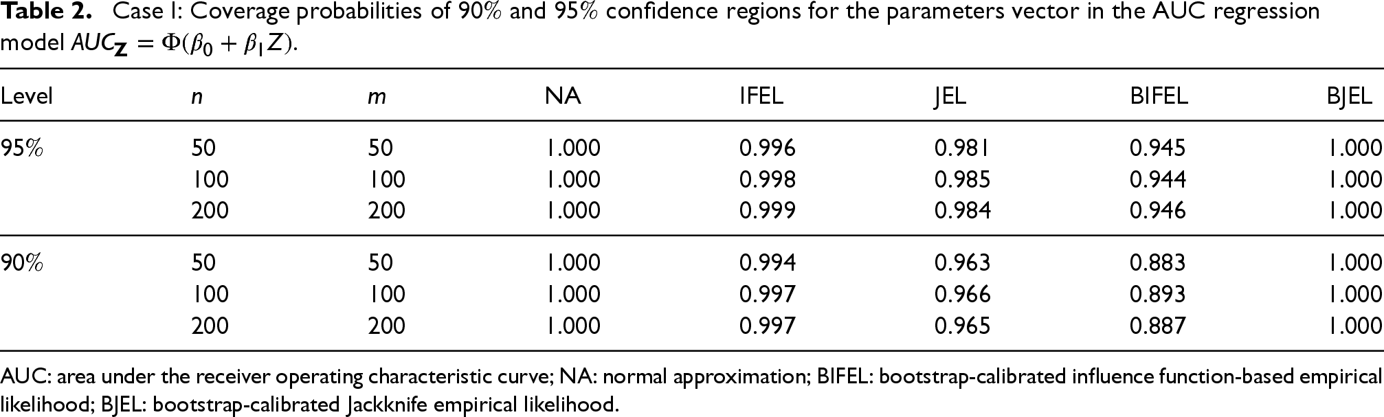
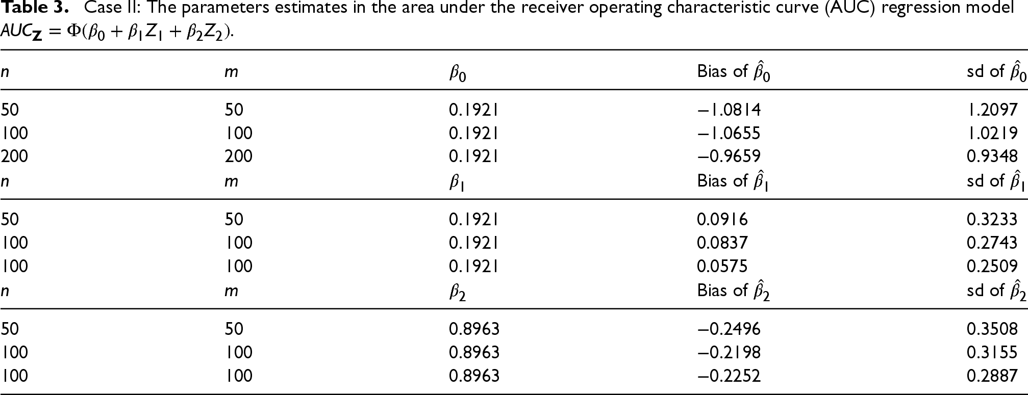
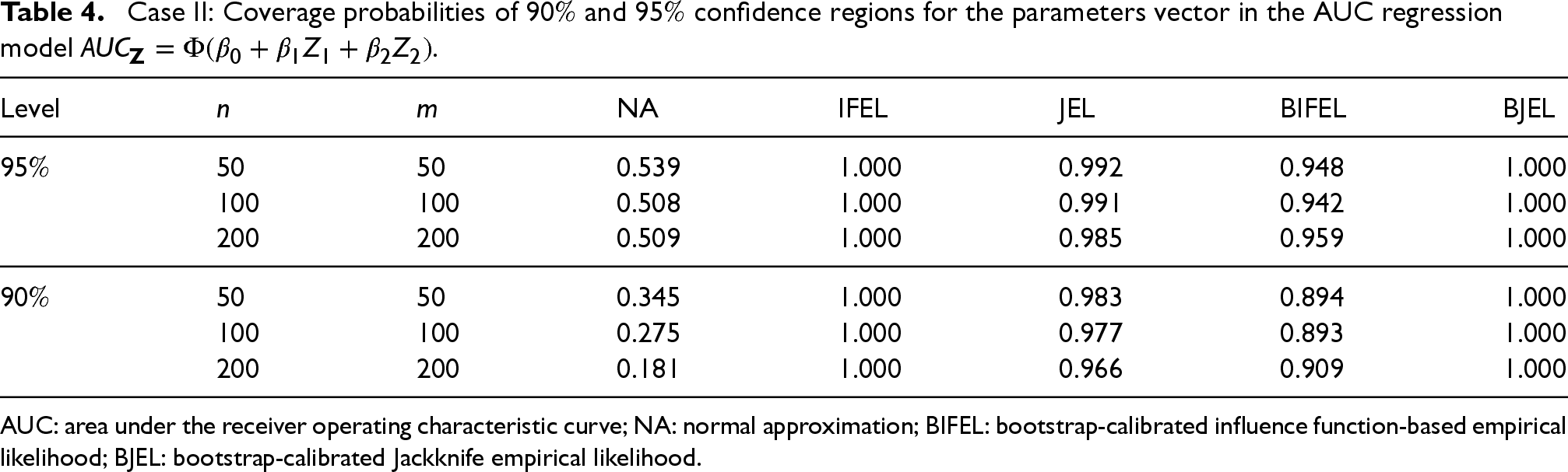
We carry out simulation studies with sample sizes $m = n$ = $50, 100, 200$ for both diseased group and non-diseased group, respectively. By generating 1000 random samples based on the above simulation settings and using estimation method for the GLM, we estimate $\hat{β}$ and calculate the coverage probabilities of the NA, IFEL, BIFEL, JEL and BJEL confidence regions for $β$ . Here $B = 200$ is used for the bootstrap methods. The parameter estimates and the coverage probabilities for $β$ are presented in Tables 1 and 2 for Case I study and in Tables 3 and 4 for Case II study, respectively. From Table 1, it is evident that the GLM method yields accurate estimates for $β$ . Table 2 shows that the BIFEL confidence region performs the best (the coverage probabilities of the BIFEL confidence regions are closer to the nominal levels) among all the confidence regions for $β$ . The NA, IFEL, JEL and BJEL regions exhibit over-coverage problems. Bootstrap calibration (BIFEL) improves the coverage accuracy of the IFEL region. Table 3 reveals that the estimates for $β$ in Case II study exhibit larger biases and standard errors compared to the estimates in Case I study. Table 4 shows that the coverage probabilities of the NA confidence regions fall significantly below the nominal confidence levels. This poor performance of the NA method may be due to its sensitivity to the inaccurate estimates of the asymptotic variance of $\hat{β}$ . IFEL, JEL and BJEL regions also show over-coverage problems, whereas the BIFEL confidence regions demonstrate superior coverage accuracy.

Table 1.

Case I: Parametric estimates in the area under the receiver operating characteristic curve (AUC) regression model $A U C_{Z} = Φ (β_{0} + β_{1} Z)$ .

$n$	$m$	$β_{0}$	Bias of ${\hat{β}}_{0}$	sd of ${\hat{β}}_{0}$
50	50	0	$-$ 0.0246	0.3106
100	100	0	$-$ 0.0085	0.2098
200	200	0	$-$ 0.0021	0.1419
$n$	$m$	$β_{1}$	Bias of ${\hat{β}}_{1}$	sd of ${\hat{β}}_{1}$
50	50	0.3201	0.0204	0.0895
100	100	0.3201	0.0061	0.0545
100	100	0.3201	0.0022	0.0359

Table 2.

Case I: Coverage probabilities of $90 %$ and $95 %$ confidence regions for the parameters vector in the AUC regression model $A U C_{Z} = Φ (β_{0} + β_{1} Z)$ .

Level	$n$	$m$	NA	IFEL	JEL	BIFEL	BJEL
$95 %$	50	50	1.000	0.996	0.981	0.945	1.000
	100	100	1.000	0.998	0.985	0.944	1.000
	200	200	1.000	0.999	0.984	0.946	1.000
$90 %$	50	50	1.000	0.994	0.963	0.883	1.000
	100	100	1.000	0.997	0.966	0.893	1.000
	200	200	1.000	0.997	0.965	0.887	1.000

AUC: area under the receiver operating characteristic curve; NA: normal approximation; BIFEL: bootstrap-calibrated influence function-based empirical likelihood; BJEL: bootstrap-calibrated Jackknife empirical likelihood.

Table 3.

Case II: The parameters estimates in the area under the receiver operating characteristic curve (AUC) regression model $A U C_{Z} = Φ (β_{0} + β_{1} Z_{1} + β_{2} Z_{2})$ .

$n$	$m$	$β_{0}$	Bias of ${\hat{β}}_{0}$	sd of ${\hat{β}}_{0}$
50	50	0.1921	$-$ 1.0814	1.2097
100	100	0.1921	$-$ 1.0655	1.0219
200	200	0.1921	$-$ 0.9659	0.9348
$n$	$m$	$β_{1}$	Bias of ${\hat{β}}_{1}$	sd of ${\hat{β}}_{1}$
50	50	0.1921	0.0916	0.3233
100	100	0.1921	0.0837	0.2743
100	100	0.1921	0.0575	0.2509
$n$	$m$	$β_{2}$	Bias of ${\hat{β}}_{2}$	sd of ${\hat{β}}_{2}$
50	50	0.8963	$-$ 0.2496	0.3508
100	100	0.8963	$-$ 0.2198	0.3155
100	100	0.8963	$-$ 0.2252	0.2887

Table 4.

Case II: Coverage probabilities of $90 %$ and $95 %$ confidence regions for the parameters vector in the AUC regression model $A U C_{Z} = Φ (β_{0} + β_{1} Z_{1} + β_{2} Z_{2})$ .

Level	$n$	$m$	NA	IFEL	JEL	BIFEL	BJEL
$95 %$	50	50	0.539	1.000	0.992	0.948	1.000
	100	100	0.508	1.000	0.991	0.942	1.000
	200	200	0.509	1.000	0.985	0.959	1.000
$90 %$	50	50	0.345	1.000	0.983	0.894	1.000
	100	100	0.275	1.000	0.977	0.893	1.000
	200	200	0.181	1.000	0.966	0.909	1.000

Scenario 2: The link function $g$ for $A U C_{Z}$ is $\frac{1}{1 + \exp (β_{0} + β_{1} Z)}$ (a simulation setting with test results following non-normal distributions):

Under scenario 2, we generate data such that $Y^{D} | Z^{D}$ and $Y^{\bar{D}} | Z^{\bar{D}}$ follow the proportional hazard models (see G $\ddot{o}$ nen and Heller²³):

h_{D} (t | Z) = \exp (k_{0} + k_{1} Z), h_{\bar{D}} (t | Z) = \exp (γ_{1} Z)

(19)

respectively, where the covariates

Z^{D}

and

Z^{\bar{D}}

are assumed to have the common component

Z

that follows the uniform distribution

U (0, 1)

. We choose

k_{0} = - 1

k_{1} = - 2.5

, and

γ_{1} = - 1

. Then the AUC regression model is

A U C_{Z} = \frac{1}{1 + \exp (β_{0} + β_{1} Z)}

(20)

where the true parameters

β_{0} = k_{0} = - 1, β_{1} = k_{1} - γ_{1} = - 1.5

We propose the bootstrap calibration procedure to construct a confidence region for $β$ as follows. (1)

Generate $Y_{j}^{D} = - l o g (V_{j}^{D}) / \exp (k_{0} + k_{1} Z_{j})$ with $V_{j}^{D}$ being independently drawn from $U (0, 1)$ and $Z_{j}$ being independently drawn from $U (0, 1)$ , $j = 1, \dots, n$ . Similarly, generate $Y_{i}^{\bar{D}} = - l o g (V_{i}^{\bar{D}}) / \exp (γ_{1} Z_{i})$ with $V_{i}^{\bar{D}}$ generated from $U (0, 1)$ and $Z_{i}$ generated from $U (0, 1)$ , $i = 1, \dots, m$ .

(2)

Draw a bootstrap resample $V_{j}^{D *}$ ’s from $V_{j}^{D}$ ’s for the “diseased” group to get the bootstrap version $({Z_{j}}^{D}, Y_{j}^{D *})$ ’s of $({Z_{j}}^{D}, Y_{j}^{D})$ ’s, and draw a bootstrap resample $V_{i}^{\bar{D} *}$ ’s from $V_{i}^{\bar{D}}$ ’s for the “non-diseased” group to get the bootstrap version $({Z_{i}}^{\bar{D}}, Y_{i}^{\bar{D} *})$ ’s of $({Z_{i}}^{\bar{D}}, Y_{i}^{\bar{D}})$ ’s.

(3)

(4)

Repeat steps 2-3 $B$ ( $B \geq 200$ is recommended) times to obtain $B$ bootstrap copies ${l_{I F}^{* b} ({\hat{β}}^{*}), b = 1, \dots, B}$ of $l_{I F} (\hat{β})$ .

Similarly, a $(1 - α)$ level called BIFEL confidence region for $β$ can be constructed as follows:

C R_{B I F} (β) = {β : l_{I F} (β) \leq χ_{(1 - α)}}

where

χ_{(1 - α)}

is the

(1 - α)

th quantile of

{l_{I F}^{* b} ({\hat{β}}^{*}), b = 1, \dots, B}

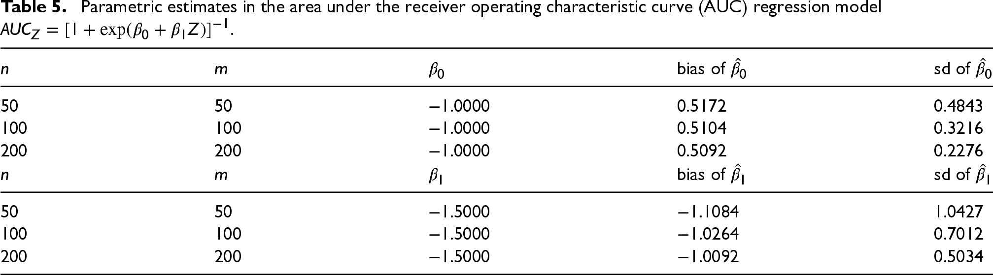
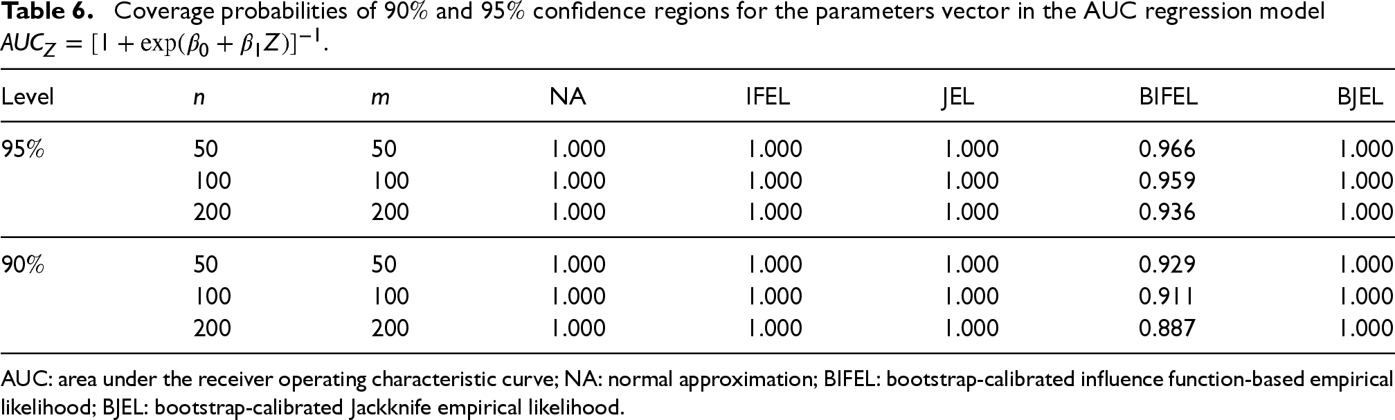
After generating data under above simulation setting in scenario 2, we can obtain estimate $\hat{β}$ for $β$ and calculate the coverage probabilities of the NA, IFEL, BIFEL, JEL and BJEL confidence regions for $β$ . The parameter estimates and the coverage probabilities for $β$ are presented in Tables 5 and 6, respectively. Table 5 shows that the GLM method provides biased estimates for $β$ with finite sample sizes. Table 6 reveals that the BIFEL confidence region achieves acceptable coverage accuracy and performs the best (the coverage probabilities of the BIFEL confidence regions are much closer to the nominal levels) among all the confidence regions for $β$ . The NA, IFEL, JEL and BJEL confidence regions suffer from over-coverage problems. Bootstrap calibration (BIFEL) greatly improves the coverage accuracy of the IFEL region.

Table 5.

Parametric estimates in the area under the receiver operating characteristic curve (AUC) regression model $A U C_{Z} = [1 + \exp (β_{0} + β_{1} Z)]^{- 1}$ .

$n$	$m$	$β_{0}$	bias of ${\hat{β}}_{0}$	sd of ${\hat{β}}_{0}$
50	50	$-$ 1.0000	0.5172	0.4843
100	100	$-$ 1.0000	0.5104	0.3216
200	200	$-$ 1.0000	0.5092	0.2276
$n$	$m$	$β_{1}$	bias of ${\hat{β}}_{1}$	sd of ${\hat{β}}_{1}$
50	50	$-$ 1.5000	$-$ 1.1084	1.0427
100	100	$-$ 1.5000	$-$ 1.0264	0.7012
200	200	$-$ 1.5000	$-$ 1.0092	0.5034

Table 6.

Coverage probabilities of $90 %$ and $95 %$ confidence regions for the parameters vector in the AUC regression model $A U C_{Z} = [1 + \exp (β_{0} + β_{1} Z)]^{- 1}$ .

Level	$n$	$m$	NA	IFEL	JEL	BIFEL	BJEL
$95 %$	50	50	1.000	1.000	1.000	0.966	1.000
	100	100	1.000	1.000	1.000	0.959	1.000
	200	200	1.000	1.000	1.000	0.936	1.000
$90 %$	50	50	1.000	1.000	1.000	0.929	1.000
	100	100	1.000	1.000	1.000	0.911	1.000
	200	200	1.000	1.000	1.000	0.887	1.000

5. Confidence interval for

A U C_{Z}

based on the BIFEL confidence region

The simulation results in Section 4 show that the bootstrap-calibrated BIFEL confidence region for $β$ outperforms the existing NA-based confidence region and other EL-based confidence regions. Therefore, we further propose an BIFEL-based confidence interval for the covariate-adjusted AUC under the AUC regression model (5) in this section. With a specified covariate $Z^{D} = Z$ , the confidence interval for the covariate-adjusted AUC can be constructed as follows:

{A U C_{Z} (β) = g (β^{T} Z) : β \in C R_{B I F} (β)}

(21)

This interval is a $(1 - α)$ level confidence interval for the covariate-adjusted AUC when $g (\cdot)$ is an one-to-one function.

Let $(q_{0}, q_{1})$ denote the confidence interval for the covariate-adjusted AUC. To compute the confidence interval, we apply the following approximation method:

\begin{aligned} q_{0} & = m i n {A U C_{Z} (β) : β \in C R_{B I F} (β)} = m i n {g (β^{T} Z^{D}) : l_{I F} (β) = c, 0 \leq c \leq χ_{(1 - α)}} \\ \approx m i n {⋃_{j = 1}^{M} (g (β^{T} Z^{D}) : l_{I F} (β) = c_{j})}, \\ q_{1} & = m a x {A U C_{Z} (β) : β \in C R_{B I F} (β)} = m a x {g (β^{T} Z^{D}) : l_{I F} (β) = c, 0 \leq c \leq χ_{(1 - α)}} \\ \approx m a x {⋃_{j = 1}^{M} (g (β^{T} Z^{D}) : l_{I F} (β) = c_{j})}, \end{aligned}

where

χ_{(1 - α)}

is the

(1 - α)

th quantile of

{l_{I F}^{* b} ({\hat{β}}^{*}), b = 1, \dots, B}

(see Section 4),

M

is a large integer number,

{c_{1}, c_{2}, \dots, c_{M}}

is a random sample of size

M

generated from the uniform distribution on

[0, χ_{(1 - α)}]

To estimate $q_{0}$ and $q_{1}$ , we use the following procedure to estimate $β$ in the first place: (1)

We approximate $C R_{B I F} (β)$ by $C R_{0} = {β : {\hat{β}}_{i} - z_{1 - α / 2} {\hat{σ}}_{i} \leq β_{i} \leq {\hat{β}}_{i} + z_{1 - α / 2} {\hat{σ}}_{i}, i = 1, 2, \dots, p}$ , where ${\hat{σ}}_{i}$ is the bootstrap standard error of ${\hat{β}}_{i}$ , and $z_{1 - α / 2}$ is the $(1 - α / 2)$ th quantile of the standard normal distribution.

(2)

For $k = 1, 2, \dots, K$ , where $K$ is a chosen integer depending on the number of regression parameters, we generate $K$ vectors ${β^{(k)} : k = 1, 2, \dots, K}$ uniformly over $C R_{0}$ satisfying $l_{I F} (β^{(k)}) \leq χ_{1 - α})$ . We can estimate $β$ to satisfy $l_{I F} (β) = c, for \forall c \in [0, χ_{1 - α}]$ using ${(β^{(k)}, l_{I F} (β^{(k)}) : k = 1, 2, \dots, K}$ .

6. A real example

In this section, we illustrate the application of the proposed method by using a dataset on prostate cancer from the Beta Carotene and Retinol Efficacy Trial (CARET).²⁴ CARET is a randomized trial conducted at the Fred Hutchinson Cancer Research Center. Prostate cancer is a malignant tumor that arises in the prostate gland, which is part of the male reproductive system. It is the second most common cancer in men worldwide. Prostate cancer is particularly prevalent in older men, with most cases occurring in those over the age of 50. Age, family history, race, and lifestyle factors (such as diet and physical activity) influence the risk of developing prostate cancer. In the study, some men had been diagnosed as having prostate cancer; some men had had at least three and up to eight bloods samples taken as long as ten years prior to diagnosis. Some of the blood samples were found to have been drawn after the diagnosis of prostate cancer and were dropped. The remaining blood samples were assayed for PSA, together with samples from age-matched controls with similar durations on study. Our CARET PSA Biomarker dataset was downloaded from the datasets in Pepe’s book website.¹ This dataset includes observations for total serum PSA of 454 subjects in controls group ( $D = 0$ ) and 229 subjects in case group ( $D = 1$ ). $Y^{D}$ or $Y^{\bar{D}}$ is the logarithm of the total serum PSA of a subject in the case group or control group. A subject’s covariates include the time $Z_{1}$ (in years, a negative value of $Z_{1}$ indicates a time before prostate cancer Dx) relative to prostate cancer Dx, and the age $Z_{2}$ of a subject. We want to know how the changes of these covariates influence the diagnostic accuracy of PSA on prostate cancer detection.

The AUC regression model used here is based on the following function:

A U C_{Z} = Φ (β_{0} + β_{1} Z_{1} + β_{2} Z_{2})

By the usual GLM-based estimation method, we obtain the estimate for the parameter vector in the AUC regression as shown in Table 7. Applying the proposed BIFEL method (with

B = 1000

), we obtain a

95 %

confidence region for the parameters vector

β

as follows:

{C R}_{B I F} (β) = {β : l_{I F} (β) \leq 0.0137}

Table 7.
Real example: Parameters estimates in $A U C_{Z} = Φ (β_{0} + β_{1} Z_{1} + β_{2} Z_{2})$ .

$\hat{β_{0}}$ $\hat{β_{1}}$ $\hat{β_{2}}$

1.2072 0.1306 0.0034

$\hat{β_{0}}$	$\hat{β_{1}}$	$\hat{β_{2}}$
1.2072	0.1306	0.0034

AUC: area under the receiver operating characteristic curve.

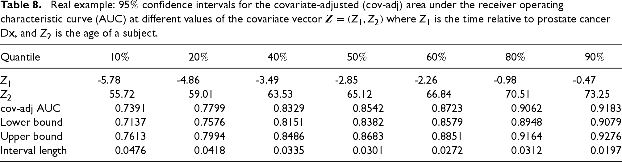
Based on this confidence region for $β$ , we can get a confidence interval for the covariate-adjusted AUC at a specified value of the covariate vector $Z^{D} = (Z_{1}, Z_{2})$ . Here, we choose $Z^{D}$ to be the $10 %, 20 %, 40 %, 50 %, 60 %, 80 %$ , and $90 %$ quantiles of the observed values for the covariate vector, and choose $K = 100$ . Table 8 presents estimates of the covariate-adjusted AUC and the corresponding $95 %$ level BIFEL intervals for the covariate-adjusted AUC at different values of $Z^{D}$ . From Table 8, we observe that the covariate-adjusted AUC of PSA is 0.7391 for men with age of 55.72 (approximately 56) and time relative to prostate cancer Dx of $-$ 5.78 years (i.e., approximately 6 years before prostate cancer Dx), and the corresponding 95% level confidence interval is $(0.7137, 0.7613)$ , which indicate that PSA has a moderate diagnostic accuracy on prostate cancer for this group of men. The covariate-adjusted AUC of PSA is 0.9062 for men with age of 70.51 (approximately 71) and time relative to prostate cancer Dx of $-$ 0.98 years (i.e., approximately 1 year before prostate cancer Dx), and the corresponding 95% level confidence interval is $(0.8948, 0.9164)$ , which indicate that PSA has a high diagnostic accuracy on prostate cancer for this group of men. Table 8 also shows that as men get older (from 56 to 73), and the time relative to prostate cancer Dx is shorter (from $-$ 5.78 to $-$ 0.47), the overall diagnostic accuracy of PSA on prostate cancer become higher (the covariate-adjusted AUC increases from 0.7391 to 0.9183). For comparison, the AUC and its $95 %$ confidence interval are calculated without covariate adjustment, which are 0.8381 and (0.8046, 0.8695), respectively. This real example shows that the PSA test has a moderate to high diagnostic accuracy for men with different covariate information, and the PSA test is an important screening tool to detect early signs of prostate cancer in asymptomatic men.

Table 8.

Real example: $95 %$ confidence intervals for the covariate-adjusted (cov-adj) area under the receiver operating characteristic curve (AUC) at different values of the covariate vector $Z = (Z_{1}, Z_{2})$ where $Z_{1}$ is the time relative to prostate cancer Dx, and $Z_{2}$ is the age of a subject.

Quantile	$10 %$	$20 %$	$40 %$	$50 %$	$60 %$	$80 %$	$90 %$
$Z_{1}$	$-$ 5.78	$-$ 4.86	$-$ 3.49	$-$ 2.85	$-$ 2.26	$-$ 0.98	$-$ 0.47
$Z_{2}$	55.72	59.01	63.53	65.12	66.84	70.51	73.25
cov-adj AUC	0.7391	0.7799	0.8329	0.8542	0.8723	0.9062	0.9183
Lower bound	0.7137	0.7576	0.8151	0.8382	0.8579	0.8948	0.9079
Upper bound	0.7613	0.7994	0.8486	0.8683	0.8851	0.9164	0.9276
Interval length	0.0476	0.0418	0.0335	0.0301	0.0272	0.0312	0.0197

7. Discussion and conclusion

Dodd and Pepe¹¹ proposed a direct modeling method for AUC in presence of covariates. While their approach allows for constructing a NA-based confidence region for the vector of the regression coefficients in the AUC regression, but the NA-based confidence region can have poor coverage accuracy (possibly due to the poor asymptotic variance estimation and/or the biased estimates for the regression vector with finite sample sizes). In this article, we introduce a new IFEL for inference on AUC in presence of covariates. Our method demonstrates favorable theoretical properties and, through the simulation results, indicates that the proposed BIFEL confidence region with bootstrap calibration outperforms the existing NA-based confidence region in terms of coverage probability. Additionally, We propose an interval estimation method for the covariate-adjusted AUC based on the BIFEL confidence region. The proposed method is an important contribution for constructing confidence intervals for the covariate-adjusted AUC. The proposed method has been applied to a real PSA Biomarker dataset. In the real data example we have found that the diagnostic accuracy of the PSA test on prostate cancer is higher as men get older and the time relative to prostate cancer Dx is shorter. This real data application indicates that the PSA test has a moderate to high diagnostic accuracy for men with different covariate information, and the PSA test is an important screening tool for detection of early signs of prostate cancer in asymptomatic men.

Footnotes

Acknowledgments

The author(s) are thankful to the anonymous referees for their helpful suggestions and comments.

Declaration of conflicting interests

The author(s) declared no potential conflicts of interest with respect to the research, authorship, and/or publication of this article.

Funding

The author(s) received no financial support for the research, authorship, and/or publication of this article.

ORCID iD

Gengsheng Qin

Appendix

In this appendix, we provide the proof of Theorem 1. For better presentation of the proof, we re-write the notations for $H_{j}$ ’s and ${\hat{H}}_{j}$ ’s (see (7) and (9) in Section 3) here:

\begin{aligned} H_{j} = (1 - U_{j}^{D} - g (β^{T} Z_{j}^{D})) ω (β^{T} Z_{j}^{D}) Z_{j}^{D}, \\ {\hat{H}}_{j} = (1 - {\hat{U}}_{j}^{D} - g (β^{T} Z_{j}^{D})) ω (β^{T} Z_{j}^{D}) Z_{j}^{D} \end{aligned}

where

U_{j}^{D} = 1 - F_{Z^{\bar{D}}}^{\bar{D}} (Y_{j}^{D})

{\hat{U}}_{j}^{D} = 1 - {\hat{F}}_{Z^{\bar{D}}}^{\bar{D}} (Y_{j}^{D})

, for

j = 1, \dots, n

, and

{\hat{F}}_{Z^{\bar{D}}}^{\bar{D}}

is the empirical estimate for

F_{Z^{\bar{D}}}^{\bar{D}}

We denote $x^{\otimes 2} = x x^{T},$ for $x \in R^{p},$ and denote $∥ \cdot ∥$ the Euclidean norm. Lemma 1 and 2 are needed for the proof of Theorem 1. Lemma 1

If $max_{j} ‖ Z_{j}^{D} ‖ = o_{p} (n^{1 / 2})$ , $lim_{n, m \to \infty} \frac{n}{m} = ρ > 0$ , the link function $g$ and the weight function $ω$ are bounded functions, then

\frac{1}{\sqrt{n + m}} \sum_{k = 1}^{n + m} W_{k} (β) \overset{L}{⟶} N (0, \frac{ρ}{1 + ρ} V)

where

\begin{aligned} W_{k} (β) & = {\begin{array}{cccc} H_{k}, & if k = 1, \dots, n, \\ ρ A (β) \int (I (Y_{k} \leq t) - F_{Z^{\bar{D}}}^{\bar{D}} (t)) d F_{Z^{D}}^{D} (t), & if k = n + 1, \dots, n + m \end{array} \\ A (β) & = lim_{n \to \infty} \frac{1}{n} \sum_{j = 1}^{n} ω (β^{T} Z_{j}^{D}) Z_{j}^{D}, \\ V & = V_{1} + V_{2}, \\ V_{1} & = A (β)^{\otimes 2} V a r_{Z^{D}}^{D} [F_{Z^{\bar{D}}}^{\bar{D}} (Y^{D})], \\ V_{2} & = ρ A (β)^{\otimes 2} V a r_{Z^{\bar{D}}}^{\bar{D}} [\int I (Y^{\bar{D}} \leq t) d F_{Z^{D}}^{D} (t)] \end{aligned}

Proof.

From the notations for $H_{j}$ ’s and ${\hat{H}}_{j}$ ’s, we obtain the following decomposition:

\frac{1}{\sqrt{n}} \sum_{j = 1}^{n} {\hat{H}}_{j} = \frac{1}{\sqrt{n}} \sum_{j = 1}^{n} H_{j} + \frac{1}{\sqrt{n}} \sum_{j = 1}^{n} (U_{j}^{D} - {\hat{U}}_{j}^{D}) ω (β^{T} Z_{j}^{D}) Z_{j}^{D} \equiv I_{1} + I_{2}

From

\begin{aligned} V a r (I_{1}) & = \frac{1}{n} V a r (\sum_{j = 1}^{n} [F_{Z_{\bar{D}}}^{\bar{D}} (Y_{j}^{D}) - g (β^{T} Z_{j}^{D})] ω (β^{T} Z_{j}^{D}) Z_{j}^{D}) \\ = \frac{1}{n} \sum_{j = 1}^{n} {(ω (β^{T} Z_{j}^{D}) Z_{j}^{D})}^{\otimes 2} V a r_{Z^{D}}^{D} [F_{Z_{\bar{D}}}^{\bar{D}} (Y_{j}^{D})] \\ ⟶ V_{1} \end{aligned}

(If

Z_{j}^{D}

’s are i.i.d. random variables, then

V_{1} = E ({(ω (β^{T} Z^{D}) Z^{D})}^{\otimes 2} V a r_{Z^{D}}^{D} [F_{Z^{\bar{D}}}^{\bar{D}} (Y^{D})])

), and Central Limit Theorem, it follows that

I_{1} \overset{L}{⟶} N (0, V_{1}) .

For the term $I_{2}$ , using ${\hat{F}}_{Z^{\bar{D}}}^{\bar{D}} (t) = \frac{1}{m} \sum_{i = 1}^{m} I (Y_{i}^{\bar{D}} \leq t)$ , we get that

\begin{aligned} I_{2} & = \frac{1}{\sqrt{n}} \sum_{j = 1}^{n} ({\hat{F}}_{Z^{\bar{D}}}^{\bar{D}} (Y_{j}^{D}) - F_{Z^{\bar{D}}}^{\bar{D}} (Y_{j}^{D})) ω (β^{T} Z_{j}^{D}) Z_{j}^{D} \\ = [lim_{n \to \infty} \frac{1}{n} \sum_{j = 1}^{n} ω (β^{T} Z_{j}^{D}) Z_{j}^{D}] \int \sqrt{n} ({\hat{F}}_{Z^{\bar{D}}}^{\bar{D}} (t) - F_{Z^{\bar{D}}}^{\bar{D}} (t)) d F_{Z^{D}}^{D} (t) + o_{p} (1) \\ = \sqrt{\frac{n}{m}} [lim_{n \to \infty} \frac{1}{n} \sum_{j = 1}^{n} ω (β^{T} Z_{j}^{D}) Z_{j}^{D}] \\ \times \sqrt{m} (\frac{1}{m} \sum_{i = 1}^{m} \int I (Y_{i}^{\bar{D}} \leq t) d F_{Z^{D}}^{D} (t) - \int F_{Z^{\bar{D}}}^{\bar{D}} (t) d F_{Z^{D}}^{D} (t)) + o_{p} (1) \\ \overset{L}{⟶} N (0, V_{2}) \end{aligned}

For given covariates $Z_{j}^{D}$ ’s, test results $Y_{j}^{D}$ ’s for the diseased group and $Y_{i}^{\bar{D}}$ ’s for the non-diseased group are independent, so $I_{1}$ and $I_{2}$ are asymptotically independent. Therefore, (A.1)

\frac{1}{\sqrt{n}} \sum_{j = 1}^{n} {\hat{H}}_{j} = I_{1} + I_{2} \overset{L}{⟶} N (0, V)

where

V = V_{1} + V_{2}

We have that (A.2)

\begin{aligned} \frac{1}{\sqrt{n + m}} \sum_{j = 1}^{n} {\hat{H}}_{j} & = \frac{1}{\sqrt{n + m}} \sum_{j = 1}^{n} H_{j} + \frac{n}{m} [lim_{n \to \infty} \frac{1}{n} \sum_{j = 1}^{n} ω (β^{T} Z_{j}^{D}) Z_{j}^{D}] \\ \times \frac{1}{\sqrt{n + m}} \sum_{i = 1}^{m} (\int I (Y_{i}^{\bar{D}} \leq t) d F_{Z^{D}}^{D} (t) - \int F_{Z^{\bar{D}}}^{\bar{D}} (t) d F_{Z^{D}}^{D} (t)) + o_{p} (1) \\ = \frac{1}{\sqrt{n + m}} \sum_{j = 1}^{n} H_{j} + \frac{ρ A (β)}{\sqrt{n + m}} \sum_{i = 1}^{m} \int (I (Y_{i}^{\bar{D}} \leq t) - F_{Z^{\bar{D}}}^{\bar{D}} (t)) d F_{Z^{D}}^{D} (t) + o_{p} (1) \\ \equiv \frac{1}{\sqrt{n + m}} \sum_{j = 1}^{n} H_{j} + \frac{1}{\sqrt{n + m}} \sum_{i = 1}^{m} ρ A (β) B_{i} + o_{p} (1) \\ \equiv \frac{1}{\sqrt{n + m}} \sum_{k = 1}^{n + m} W_{k} (β) + o_{p} (1) \end{aligned}

where

B_{i} = \int (I (Y_{i}^{\bar{D}} \leq t) - F_{Z^{\bar{D}}}^{\bar{D}} (t)) d F_{Z^{D}}^{D} (t)

Lemma 1 follows immediately from (A.1), (A.2) and

\frac{1}{\sqrt{n + m}} \sum_{k = 1}^{n + m} W_{k} (β) = \sqrt{\frac{n}{n + m}} \frac{1}{\sqrt{n}} \sum_{j = 1}^{n} {\hat{H}}_{j} + o_{p} (1) .

Lemma 2

If $max_{j} ‖ Z_{j}^{D} ‖ = o_{p} (n^{1 / 2})$ , $lim_{n, m \to \infty} \frac{n}{m} = ρ > 0$ , the link function $g$ and the weight function $ω$ are bounded functions, then we have that

\begin{aligned} (i) & max_{k} ∥ {\hat{W}}_{k} (β) ∥ = o_{p} (N^{1 / 2}), \\ (i i) & \frac{1}{N} \sum_{j = 1}^{N} {\hat{W}}_{k} (β)^{\otimes 2} \overset{p}{⟶} \frac{ρ}{1 + ρ} V \end{aligned}

where

N = n + m

Proof.

(i) Under the condition that $max_{j} ‖ Z_{j}^{D} ‖ = o_{p} (n^{1 / 2})$ , we have $max_{j} ∥ H_{j} ∥= o_{p} (n^{1 / 2}) .$ From $sup_{y} | \sqrt{n} ({\hat{F}}_{Z^{\bar{D}}}^{\bar{D}} (y) - F_{Z^{\bar{D}}}^{\bar{D}} (y)) | = O_{p} (1)$ , it follows that

\begin{aligned} ‖ {\hat{H}}_{j} - H_{j} ‖ & = ‖ (U_{j}^{D} - {\hat{U}}_{j}^{D}) ω (β^{T} Z_{j}^{D}) Z_{j}^{D} ‖ \\ = | {\hat{F}}_{Z^{\bar{D}}}^{\bar{D}} (Y_{j}^{D}) - F_{Z^{\bar{D}}}^{\bar{D}} (Y_{j}^{D}) | ‖ ω (β^{T} Z_{j}^{D}) Z_{j}^{D} ‖ \\ \leq sup_{y} | {\hat{F}}_{Z^{\bar{D}}}^{\bar{D}} (y) - F_{Z^{\bar{D}}}^{\bar{D}} (y) | ‖ ω (β^{T} Z_{j}^{D}) Z_{j}^{D} ‖ = o_{p} (1) \end{aligned}

uniformly for

j = 1, 2, \dots, n

. Therefore,

max_{j} ∥ {\hat{H}}_{j} ∥ \leq max_{j} ∥ H_{j} ∥ + max_{j} ∥ {\hat{H}}_{j} - H_{j} ∥ = o_{p} (n^{1 / 2})

Hence,

max_{k} ∥ {\hat{W}}_{k} (β) ∥ \leq max_{k} ∥ {\hat{H}}_{k} ∥ + C max_{k} ∥ Z_{k}^{D} ∥ = o_{p} (N^{1 / 2})

where

C

is a generic constant.

(ii) From $sup_{y} | \sqrt{n} ({\hat{F}}_{Z^{\bar{D}}}^{\bar{D}} (y) - F_{Z^{\bar{D}}}^{\bar{D}} (y)) | = O_{p} (1)$ , and $sup_{y} | \sqrt{n} ({\hat{F}}_{Z^{D}}^{D} (y) - F_{Z^{D}}^{D} (y)) | = O_{p} (1)$ , we have that (A.3)

\begin{aligned} max_{k} ∥ {\hat{W}}_{k} (β) - W_{k} (β) ∥ \leq max_{j} ∥ {\hat{H}}_{j} - H_{j} ∥ \\ + C max_{k} | \int (I (Y_{k} \leq t) - {\hat{F}}_{Z^{\bar{D}}}^{\bar{D}} (t)) d {\hat{F}}_{Z^{D}}^{D} (t) - \int (I (Y_{k} \leq t) - F_{Z^{\bar{D}}}^{\bar{D}} (t)) d F_{Z^{D}}^{D} (t) | + o_{p} (1) \\ = o_{p} (1) \end{aligned}

From the proof of Lemma 1, it follows that

(A.4)

\begin{aligned} \frac{1}{N} \sum_{j = 1}^{N} W_{k} (β)^{\otimes 2} & = \frac{1}{N} \sum_{j = 1}^{n} H_{j}^{\otimes 2} + \frac{1}{N} \sum_{i = 1}^{m} ρ^{2} A (β)^{\otimes 2} B_{i}^{2} \end{aligned}

(A.5)

\begin{aligned} \overset{p}{⟶} \frac{ρ}{1 + ρ} E (H_{1}^{\otimes 2}) + \frac{ρ}{1 + ρ} \cdot ρ A (β)^{\otimes 2} E (B_{1}^{2}) \end{aligned}

(A.6)

\begin{aligned} = \frac{ρ}{1 + ρ} (V_{1} + V_{2}) = \frac{ρ}{1 + ρ} V \end{aligned}

Lemma 2 (ii) follows from (A.3) and (A.6) right away.

Proof. The Proof of Theorem 1.

Using Lemma 1, Lemma 2 (ii) and the similar argument used in Owen,¹⁶ we can prove that (A.7)

∥ ν ∥ = O_{p} (N^{- 1 / 2})

Then, applying Taylor’s expansion, we get that

\begin{aligned} l_{I F} (β_{0}) & = 2 \sum_{k = 1}^{N} \log (1 + ν^{T} {\hat{W}}_{k} (β)) \\ = 2 \sum_{k = 1}^{N} (ν^{T} {\hat{W}}_{k} (β) - \frac{1}{2} (ν^{T} {\hat{W}}_{k} (β))^{2}) + r_{1 N} \end{aligned}

with

| r_{1 N} | \leq C \sum_{k = 1}^{N} | ν^{T} {\hat{W}}_{k} (β) |^{3} \leq C ∥ ν ∥^{3} max_{j} ∥ {\hat{W}}_{k} (β) ∥ \sum_{j} ∥ {\hat{W}}_{k} (β) ∥^{2} = o_{p} (1)

By (11), we have (A.8)

\begin{aligned} \sum_{k = 1}^{N} \frac{{\hat{W}}_{k} (β)}{1 + ν^{T} {\hat{W}}_{k} (β)} = & \sum_{k = 1}^{N} {\hat{W}}_{k} (β) [1 - ν^{T} {\hat{W}}_{k} (β) + \frac{(ν {\hat{W}}_{k} (β))^{2}}{1 + ν^{T} {\hat{W}}_{k} (β)}] \\ = & \sum_{k = 1}^{N} {\hat{W}}_{k} (β) - (\sum_{k = 1}^{N} {\hat{W}}_{k} (β)^{\otimes 2}) ν + \sum_{k = 1}^{N} \frac{{\hat{W}}_{k} (β) {(ν^{T} {\hat{W}}_{k} (β))}^{2}}{1 + ν^{T} {\hat{W}}_{k} (β)} = 0 \end{aligned}

(A.7), (A.8) and Lemma 2 together imply that

ν = {(\sum_{k = 1}^{N} {\hat{W}}_{k} (β)^{\otimes 2})}^{- 1} \sum_{k = 1}^{N} {\hat{W}}_{k} (β) + o_{p} (N^{- 1 / 2})

Again by (11), we get that (A.9)

\begin{aligned} 0 = \sum_{k = 1}^{N} \frac{ν^{T} {\hat{W}}_{k} (β)}{1 + ν^{T} {\hat{W}}_{k} (β)} = & \sum_{k = 1}^{N} (ν^{T} {\hat{W}}_{k} (β)) [1 - ν^{T} {\hat{W}}_{k} (β) + \frac{(ν^{T} {\hat{W}}_{k} (β))^{2}}{1 + ν^{T} {\hat{W}}_{k} (β)}] \\ = & \sum_{k = 1}^{N} (ν^{T} {\hat{W}}_{k} (β)) - \sum_{k = 1}^{N} {(ν^{T} {\hat{W}}_{k} (β))}^{2} + \sum_{k = 1}^{N} \frac{{(ν^{T} {\hat{W}}_{k} (β))}^{3}}{1 + ν^{T} {\hat{W}}_{k} (β)} \end{aligned}

From (A.7) and Lemma 2, we can get

\frac{1}{n} \sum_{k = 1}^{N} \frac{{(ν^{T} {\hat{W}}_{k} (β))}^{3}}{1 + ν^{T} {\hat{W}}_{k} (β)} = o_{p} (1)

then we get (A.10)

\sum_{k = 1}^{N} ν {\hat{W}}_{k} (β) = \sum_{k = 1}^{N} (ν {\hat{W}}_{k} (β))^{2} + o_{p} (1)

From (A.7)–(A.10), Lemma 1, and Lemma 2 (ii), it follows that

\begin{aligned} l_{I F} (β_{0}) & = \sum_{k = 1}^{N} ν^{T} {\hat{W}}_{k} (β)^{\otimes 2} ν + o_{p} (1) \\ = {(\frac{1}{\sqrt{N}} \sum_{k = 1}^{N} {\hat{W}}_{k} (β))}^{T} {(\frac{1}{N} \sum_{k = 1}^{N} {\hat{W}}_{k} (β)^{\otimes 2})}^{- 1} (\frac{1}{\sqrt{N}} \sum_{k = 1}^{N} {\hat{W}}_{k} (β)) + o_{p} (1) \\ \overset{L}{⟶} χ_{p}^{2} \end{aligned}

References

Pepe

. The statistical evaluation of medical tests for classification and prediction. New York: Oxford University Press, 2003.

Cohen

Korevaar

Altman

, et al. STARD 2015 guidelines for reporting diagnostic accuracy studies: explanation and elaboration. BMJ Open 2016; 6: e012799.

de Carvalho

Jara

Hanson

, et al. Bayesian nonparametric ROC regression modeling. Bayesian Anal 2013; 8: 623–646.

Henderson

Eastham

Culkin

, et al. Prostate-specific antigen (PSA) and PSA density: racial differences in men without prostate cancer. J Natl Cancer Inst 1997; 89: 134–138.

Sanda

Feng

Howard

, et al. Association between combined TMPRSS2: ERG and PCA3 RNA urinary testing and detection of aggressive prostate cancer. JAMA Oncol 2017; 3: 1085–1093.

Partin

Catalona

Southwick

, et al. Analysis of percent free prostate-specific antigen (PSA) for prostate cancer detection: influence of total PSA, prostate volume, and age. Urology 1996; 48: 55–61.

Lee

van Es

Takada

, et al. Covariate-specific ROC curve analysis can accommodate differences between covariate subgroups in the evaluation of diagnostic accuracy. J Clin Epidemiol 2023; 160: 14–23.

Thompson

Zucchini

. On the statistical analysis of ROC curves. Stat Med 1989; 8: 1277–1290.

Obuchowski

. Multireader, multimodality receiver operating characteristic curve studies: hypothesis testing and sample size estimation using analysis of variance approach with dependent observations. Acad Radiol 1995; 2: S22–S29.

10.

Dorfman

Berbaum

Metz

. Receiver operating characteristic analysis: generalization to the population of readers and patients with the jackknife method. Stat Radiol 1992; 27: 723–731.

11.

Dodd

Pepe

. Semi-parametric regression for the area under the receiver operating characteristic curve. J Am Stat Assoc 2003; 98: 409–417.

12.

Dodd

Pepe

. Partial AUC estimation and regression. Biometrics 2003; 59: 614–623.

13.

Liu

Zhou

. Covariate adjustment in estimating the area under ROC curve with partially missing gold standard. Biometrics 2013; 69: 91–100.

14.

Meng

Tubbs

. Application of a beta regression model for covariate adjusted ROC. Curr Res Biostat 2020 2024; 10: 20–24.

15.

Owen

. Empirical likelihood ratio confidence intervals for single functional. Biometrika 1988; 75: 237–249.

16.

Owen

. Empirical likelihood ratio confidence regions. Ann Stat 1990; 18: 90–120.

17.

Hall

La Scala

. Methodology and algorithms of empirical likelihood. Int Stat Rev 1990; 58: 109–127.

18.

Owen

. Empirical likelihood. New York: Chapman and Hall/CRC, 2001.

19.

Claeskens

Jing

Peng

, et al. Empirical likelihood confidence regions for comparison distributions and ROC curves. Canad J Stat 2003; 31: 173–190.

20.

Qin

Zhou

. Empirical likelihood inference for the area under the ROC curve. Biometrics 2006; 62: 613–622.

21.

Pepe

Cai

. The analysis of placement values for evaluating discriminatory measures. Biometrics 2004; 60: 528–535.

22.

Jing

Yuan

Zhou

. Jackknife empirical likelihood. J Am Stat Assoc 2009; 104: 1224–1232.

23.

Gönen

Heller

. Lehmann family of ROC curves. Med Decis Making 2010; 30: 509–517.

24.

Thornquist

Omenn

Goodman

, et al. Statistical design and monitoring of the carotene and retinol efficacy trial. Control Clin Trials 1993; 14: 308–324.

Influence function-based empirical likelihood for area under the receiver operating characteristic curve in presence of covariates

Abstract

Keywords

1. Introduction

2. Direct modeling and inference for AUC in presence of covariates

3.1. Confidence region of β based on IFEL method

Table 7. Real example: Parameters estimates in A U C Z = Φ ( β 0 + β 1 Z 1 + β 2 Z 2 ) . β 0 ^ β 1 ^ β 2 ^ 1.2072 0.1306 0.0034

Footnotes

Acknowledgments

Declaration of conflicting interests

Funding

ORCID iD

Appendix

References

3.1. Confidence region of $β$ based on IFEL method

Table 7.
Real example: Parameters estimates in $A U C_{Z} = Φ (β_{0} + β_{1} Z_{1} + β_{2} Z_{2})$ .

$\hat{β_{0}}$ $\hat{β_{1}}$ $\hat{β_{2}}$

1.2072 0.1306 0.0034