Semiparametric estimator for the covariate-specific receiver operating characteristic curve

Abstract

The study of the predictive ability of a marker is mainly based on the accuracy measures provided by the so-called confusion matrix. Besides, the area under the receiver operating characteristic curve has become a popular index for summarizing the overall accuracy of a marker. However, the nature of the relationship between the marker and the outcome, and the role that potential confounders play in this relationship could be fundamental in order to extrapolate the observed results. Directed acyclic graphs commonly used in epidemiology and in causality, could provide good feedback for learning the possibilities and limits of this extrapolation applied to the binary classification problem. Both the covariate-specific and the covariate-adjusted receiver operating characteristic curves are valuable tools, which can help to a better understanding of the real classification abilities of a marker. Since they are strongly related with the conditional distributions of the marker on the positive (subjects with the studied characteristic) and negative (subjects without the studied characteristic) populations, the use of proportional hazard regression models arises in a very natural way. We explore the use of flexible proportional hazard Cox regression models for estimating the covariate-specific and the covariate-adjusted receiver operating characteristic curves. We study their large- and finite-sample properties and apply the proposed estimators to a real-world problem. The developed code (in R language) is provided on Supplemental Material.

Keywords

Binary classification problem covariate-specific receiver operating characteristic curve covariate-adjusted receiver operating characteristic curve semiparametric estimator

1. Introduction

The receiver operating characteristic (ROC) curve¹ is routinely used for evaluating the performance of a continuous marker as diagnostic or prognostic tool. Conventionally, the (pooled) ROC curve depicts, for each potential threshold, $c \in R$ , the rate of positive subjects (those with the characteristic/disease under study) correctly classified as positive (their marker values are greater than $c$ ), or sensitivity, against the rate of negative subjects (those without the characteristic/healthy) incorrectly classified as positive (their marker values are also greater than $c$ ), that is, 1–specificity. Besides, the area under this curve,² AUC, has become a popular index for determining the association level between continuous variables and binary outcomes.³

When we measure the marker performance, the emphasis is often placed on accuracy, and we are not worried about the nature of the relationship between the marker and the outcome, or the potential interference that covariates could have on this relationship. However, this can be a crucial component in the correct practical implementation of the obtained results. For instance, Yala et al.⁴ considered different mammography-based breast cancer risk models. On a cohort including 8751 examinations and 269 cancers (at 5 years), the Tyrer-Cuzick (TC) model⁵ reported an AUC of 0.62 (95% confidence interval of 0.57–0.66). Considering the 3157 patients who were white (7107 examinations; 233 cancers) the AUC was essentially the same, 0.62 (0.57–0.67). However, on the 202 patients who were African-American (424 examinations; 11 cancers) the AUC was only 0.45 (0.21–0.66). In this case, the modest classification capacity reported by the TC model, mostly computed in white women, totally disappears when we apply the model to African-American women. Besides, the overall (pooled) AUC does not reflect the correct weighted average of those AUCs (0.61), and the poor behavior of the procedure in this small subpopulation is totally diluted. In this context, the covariate-specific and the covariate-adjusted ROC curves arise as valuable tools for depicting the real diagnostic accuracy of a marker taking into account the relevant information provided by the covariates.

Recall that the pooled ROC curve describes the performance of classification rules based on the same thresholds for each subject. That is, the thresholds are independent of the covariate value of each particular subject. As we saw previously, the consequence of this classification is that, when the covariate is associated with both the marker and the binary outcome, the marker should be calibrated to account for this covariate (see, Janes and Pepe⁶ for a deeper discussion about the need of adjusting for covariates in studies of diagnostic, screening, or prognostic markers). The covariate-specific ROC curve is the standard ROC curve conditioned on a specific covariate value. That is, it describes the diagnostic accuracy of the studied marker in the subpopulation determined by each covariate value. It describes the accuracy of the marker when covariate-specific thresholds are used for selecting the classification rules. Mathematically, let $[ξ | D = d]$ be the random variable modeling the behavior of the studied marker in the positive ( $d = 1$ ), and in the negative ( $d = 0$ ) populations. Let $X$ be a k-dimensional random variable modeling the behavior of the vector of relevant covariates. For each $x$ in the domain of $X$ and $t \in [0, 1]$ , the conditional or covariate-specific ROC curve is defined by the following equation:

R (t | x) = 1 - F_{1} (F_{0}^{- 1} (1 - t | x) | x)

(1)

where

F_{d} (\cdot | x) = P {ξ \leq \cdot | D = d, X = x}

(

d \in {0, 1}

). Notice that, from a practical point of view, it only makes sense to consider those values of

x

within the intersection of the supports of both

X_{D_{0}} = [X ∣ D = 0]

and

X_{D_{1}} = [X ∣ D = 1]

. This ROC curve must be considered when the discriminatory capacity of the diagnostic test is affected by covariates. Figure 1 depicts an example of density functions for positive and negative populations which vary with the value of the covariate, and the resulting ROC curve surface. There are situations, however, in which, despite the behavior of the test diagnostic varies with the covariates, its discriminatory capacity is not affected. In these cases, Janes and Pepe⁷ proposed to use as measure of covariate-adjusted classification accuracy the overall sensitivities when thresholds are covariate-specific. The resulting so-called covariate-adjusted ROC curve is, therefore, defined for each point

t \in [0, 1]

a R (t) = 1 - F_{1} (F_{0}^{- 1} (1 - t | X_{D_{1}}))

It is easy to check that this definition can be rewritten as follows:

a R (t) = \int R (t | x) d H_{1} (x)

(2)

where

H_{1} (\cdot) = P {X \leq \cdot | D = 1}

is the multivariate cumulative distribution function (CDF) of the covariate vector on the positive population. It is worth to highlight the predominant role that the distribution of the covariate in the positive population has in the above definition. This is consistent with the different treatment that the concepts of sensitivity and specificity have on different practical problems (for example, screening). The last definition, as it is explained by Janes and Pepe,⁷ allows to interpret the covariate-adjusted ROC curve as an overall sensitivity when the threshold used to define the test positivity is covariate-specific.

There is a number of proposals for estimating both the covariate-specific and the covariate-adjusted ROC curves. Early proposals, such as the ones by Pepe,^8,9 or Faraggi¹⁰ rely on parametric or semiparametric regression models. Fully nonparametric estimators based on nonparametric estimators of the involved conditional distribution and quantile functions were proposed by López-de-Ullibarri et al.¹¹ Pardo-Fernández et al.¹² reviewed the existing methods including covariates in the ROC analysis focusing on those employing nonparametric regression models. They classified those procedures in two categories: those modeling directly the covariate-specific ROC curve as the response of a generalized regression model (see, for instance, the proposal by Rodríguez-Alvarez et al.,¹³ where generalized additive models are considered) and those based on induced-regression methodology (e.g. the proposals by González-Manteiga et al.¹⁴ and Rodríguez-Álvarez et al.,¹⁵ where nonparametric location-scale models are employed). After the publication of this review, new estimators have been proposed in the specialized literature. For instance, Inácio de Carvalho and Rodríguez-Álvarez^16,17 proposed a highly robust model based on a combination of B-splines, dependent Dirichlet process mixture models, and the Bayesian bootstrap for the covariate-adjusted ROC curve. Recently, Bianco et al.^18,19 also focused on the robust aspects of the covariate-specific ROC curve estimation, and considered regression-induced procedures with complex covariate structures.

In this piece of research, we aim the direct estimation of the involved conditional CDFs. With this goal, we assume that the relationship between the marker on both the positive and the negative populations and the covariates follows the proportional hazard regression model proposed by Cox.²⁰ In this context, this model implies that the effect of the covariate vector is proportional along all the potential values of the marker. The already traditional strategy of using the Breslow estimator and the maximization of the partial likelihood function involving the marginal distributions of the ranks of the observed marker values²¹ is used for estimating the unknown CDFs. In order to gain flexibility in the final estimator, we let different effects and models on the two involved populations, and an adaptive regression splines function is used in order to modulate the impact of the covariate on the CDFs.

The rest of the article is organized as follows. In Section 2, both the proposed model and its semiparametric estimator are exposed. In Section 3, we explore the asymptotic properties of the resulting covariate-specific and covariate-adjusted ROC curve estimators. Finite-sample behavior of these estimators are studied via Monte Carlo simulations in Section 4, while a real-world example illustrates their practical use in Section 5. Finally, in Section 6, we present our main conclusions. Some technical issues are relegated to the Appendix. As Supplemental Material, we provide the R code used for implementing the proposed procedure and additional Monte Carlo results.

2. Semiparametric covariate-specific ROC curve estimator

2.1. The model

Let $F_{d} (\cdot | x)$ be the CDF of the marker in population $D = d$ ( $d \in {0, 1}$ with the values $0$ and $1$ representing the negative and the positive populations, respectively) conditioned to the $k$ -dimensional covariate value $X = x$ . For $y \in R$ , we assume the general proportional hazards model

\log {1 - F_{d} (y | x)} = - Λ_{d} (y | x) = - Λ_{d}^{(0)} (y) \cdot \exp {τ_{d} (x)}

(3)

where

Λ_{d}^{(0)} (\cdot)

and

τ_{d} (\cdot)

are arbitrary functions satisfying the required restrictions for letting

F_{d} (\cdot | x)

be a CDF. That is, if

λ_{d}^{(0)} (\cdot) = Λ_{d}^{(0)^{'}} (\cdot)

(derivative of

Λ_{d}^{(0)}

), then for each

x \in R^{k}

f_{d} (y | x) = λ_{d}^{(0)} (y) \cdot \exp {τ_{d} (x)} \cdot [1 - F_{d} (y | x)]

is a density function.

In this context, the proportional hazards model implies that the marker has a baseline behavior, determined by the so-called baseline cumulative risk function, $Λ_{d}^{(0)} (\cdot)$ , and that this behavior can be modified by the covariate values through the function $τ_{d} (\cdot)$ . This modification does not depend on the marker value, and has an exponential effect on the baseline distribution. Notice that, given $z$ and $x$ , two potential values of the covariate vector $X$ , based on equation (3), $F_{d} (y | z) = 1 - [1 - F_{d} (y | x}]^{\exp {τ_{d} (z) - τ_{d} (x)}}, \forall y \in R$ ( $d \in {0, 1}$ ). Although the function $τ_{d} (\cdot)$ admits a wide spectrum of possibilities, in general, the covariate effect will modify the shape of the distribution including both its mean and standard deviation. For regular $τ_{d} (\cdot)$ , bi-normal models (both the positive and negative populations are normally distributed) in which the covariate only changes the means would not fulfill the proposed model.

As usual, parametric and semi-parametric models are restrictive. The required assumptions could result unrealistic for particular practical situations. Fortunately, the literature is plenty of goodness of fit (GoF) procedures. In the context of PH Cox regression, Lin and Wei²², Grønnesby and Borgan,²³ or Parzen and Lipstsitz,²⁴ among others, have proposed specific GoF tests for the model at hand. Software implementations of some of these procedures, including several R packages, are available.

2.1.1. Examples

The survival literature is rich in proportional hazards (PH) models. The exponential distribution is the most well-known family. Distributions satisfying $\log {1 - F_{d} (y | x)} = - λ_{d}^{0} \cdot y \cdot \exp {τ_{d} (x)}$ , with $λ_{d}^{0} > 0$ and $τ_{d} (\cdot)$ an adequate function (see previous comments about $τ_{d} (\cdot)$ restrictions), are frequently used in the PH context. Figure 2 (Example 1) shows the exponential density function $f (y | x) = (x + 1)^{- 1} \cdot \exp {- y / (x + 1)}$ , for five different values of a one-dimensional covariate $x$ , which fulfills the specification in (3) by putting $λ_{d}^{0} = 1$ and $τ_{d} (x) = \log (1 / (x + 1))$ . However, the considered model is flexible enough for not just including exponential-shaped distributions. For instance, the densities $f_{d} (y | x) = \exp {τ_{d} (x)} \cdot [1 - Φ_{μ, σ} (y)]^{\exp {τ_{d} (x) - 1}} \cdot φ_{μ, σ} (y)$ , where $Φ_{μ, σ} (\cdot)$ and $φ_{μ, σ} (\cdot)$ are the CDF and probability density function (PDF) of a normal distributed variable with mean $μ$ and standard deviation $σ$ , respectively, also satisfy the PH assumption for a wide range of $τ_{d} (\cdot)$ functions. Figure 2 (Example 2) depicts these densities for $μ = 0, σ = 1$ , and $τ_{d} (x) = \log {1 + 2 \cdot x^{2}}$ , for five different values of $x$ .

Figure 1.

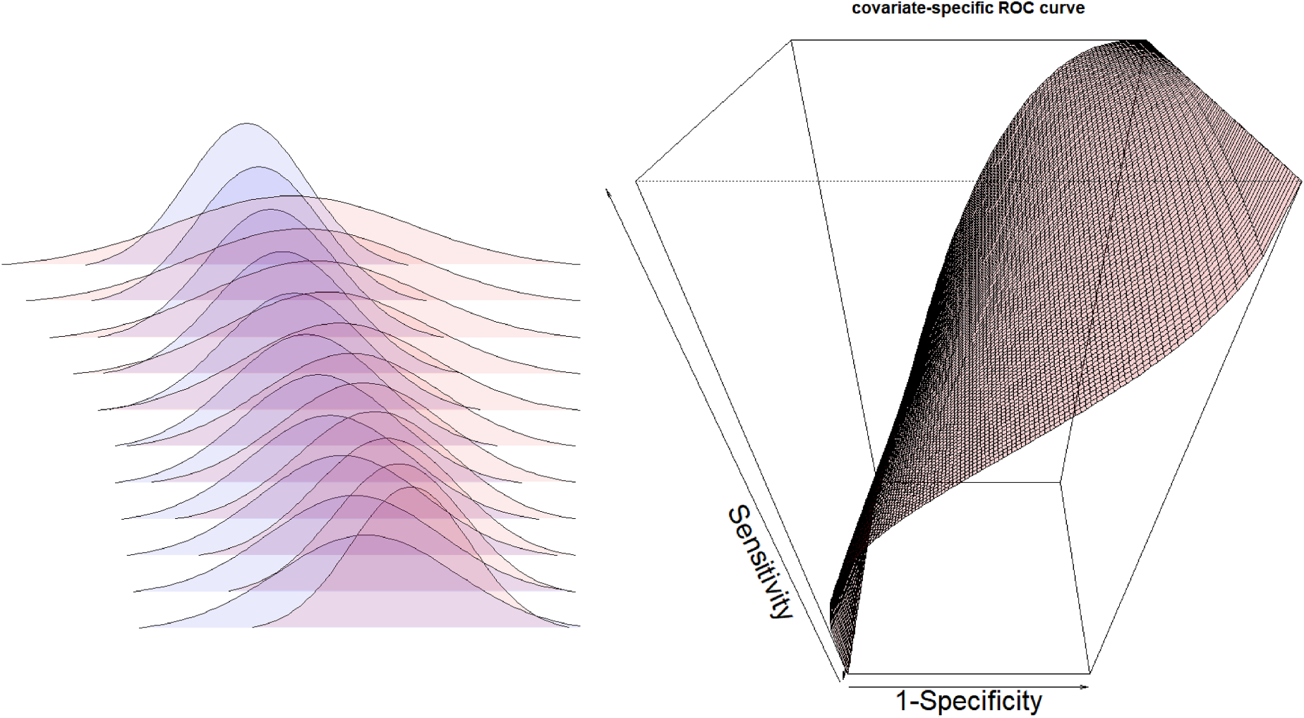
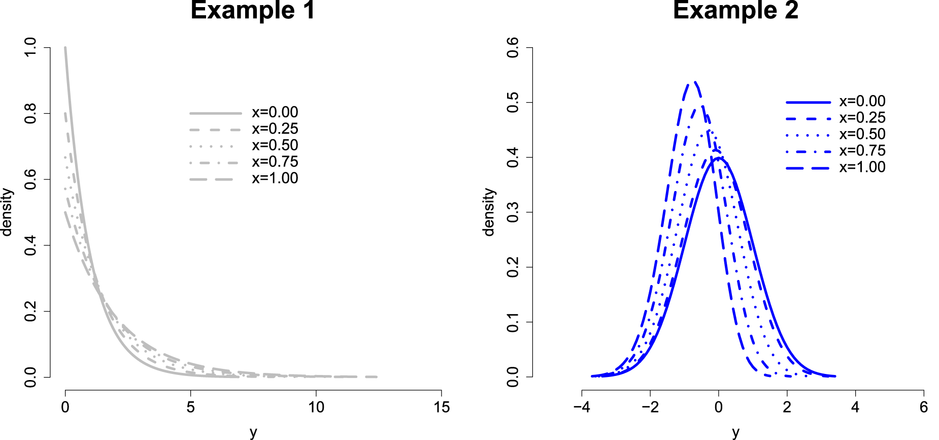
Covariate-specific receiver operating characteristic (ROC) curve. At left, density functions for the negative (following a distribution $N (0, 1.5 - (1 / 2) \cdot x)$ ) and the positive ( $N (3 / 4, 1 + x)$ ) populations, for different values of the covariate, $x \in (0, 1)$ . At right, resulting covariate-specific ROC curves.

Figure 2.

Proportional hazard (PH) examples. Example 1: Exponential density functions $f (y | x) = (x + 1)^{- 1} \cdot \exp {- y / (x + 1)}$ , for five different values of $x$ . Example 2: Density functions $f (y | x) = (1 + 2 \cdot x^{2}) \cdot [1 - Φ_{0, 1} (y)]^{2 \cdot x^{2}} \cdot φ_{0, 1} (y)$ for the same five values of $x$ .

From the standard covariate-specific ROC curve definition, under the functional restrictions of the considered model given in equation (3), we directly obtain the following alternative characterization for the covariate-specific ROC curve in terms of the involved cumulative risk functions,

\begin{aligned} \log {R (t | x)} & = - Λ_{1} (Λ_{0}^{- 1} (\log {1 / t} | x) | x) \\ = - Λ_{1}^{(0)} (Λ_{0}^{(0), - 1} (\log {1 / t} \cdot \exp {- τ_{0} (x)})) \cdot \exp {τ_{1} (x)}, t \in (0, 1) \end{aligned}

(4)

2.2. The estimator

For $d \in {0, 1}$ , let ${(y_{d, i}, x_{d, i})}_{i = 1}^{n_{d}}$ be an i.i.d. sample of observations of the $(k + 1)$ -dimensional random variable ${[ξ | D = d], [X | D = d]}$ . Let $n = n_{0} + n_{1}$ . Without loss of generality, in each population ( $d = 0$ or $d = 1$ ), we will assume that the sample is ordered according to the values of the marker, that is, $y_{d, 1} \leq y_{d, 2} \leq \dots \leq y_{d, n_{d}}$ . We assume, just for a moment, that the function $τ_{d} (\cdot)$ is known. Then, the natural estimator for the baseline cumulative risk function, $Λ_{d}^{(0)} (\cdot)$ , is given by the following equation:

{\hat{Λ}}_{d, n_{d}}^{(0)} (y) = \sum_{i = 1}^{n_{d}} {\frac{I (y_{d, i} \leq y)}{\sum_{j = i}^{n_{d}} \exp {τ_{d} (x_{d, j})}}}

(5)

where $I (\cdot)$ stands for the standard indicator function ( $I (A)$ takes the value 1 if $A$ is true, and 0 otherwise). This is the so-called Breslow or generalized Nelson-Aalen estimate. Notice that it is the Nelson-Aalen estimator when $τ_{d} (x) = 0$ , $\forall x$ . The estimator of the conditional cumulative risk function, $Λ_{d}^{(0)} (\cdot)$ , is, therefore,

{\hat{Λ}}_{d, n_{d}} (y | x) = {\hat{Λ}}_{d, n_{d}}^{(0)} (y) \cdot \exp {τ_{d} (x)}

(6)

Now, we propose to use cubic splines for approximating the function

τ_{d} (\cdot)

. A spline is a piecewise polynomial with continuity conditions on the function and its derivatives at the points where the pieces join. See, for example, Sleeper and Harrington²⁵ for an application of splines in the context of estimation of Cox models. Let

{B_{k} (\cdot)}_{k = 1}^{K}

be the usual cubic (polynomial degree)

B

-splines basis for the space of functions

F

,²⁶ where

K

is an adequate natural number depending on the dimension of the covariate vector (see Truong and Stone²⁷ for more details). We will approximate

τ_{d} (\cdot)

through a function of the form

τ_{d}^{*} (\cdot; θ_{d}) = \sum_{k = 1}^{K} θ_{d, k} \cdot B_{k} (\cdot)

, where

θ_{d} = (θ_{d, 1}, \dots, θ_{d, K})

. It is known (see, for instance, Strawderman and Tsiatis²⁸) that the maximization of the log-likelihood

ℓ (θ_{d}) = \sum_{i = 1}^{n_{d}} {λ_{d} (y_{d, i}) \cdot τ_{d}^{*} (x_{d, i}; θ_{d}) - \sum_{j = 1}^{i} λ_{d} (y_{d, j}) \cdot \exp {τ_{d}^{*} (x_{d, j}; θ_{d})}}

(7)

reports a consistent estimator, say

{\hat{θ}}_{d, n_{d}}

, for the parameter

θ_{d}

, and, therefore, the function

τ_{d}^{*} (\cdot; {\hat{θ}}_{d, n_{d}})

is a consistent estimator for

τ_{d}^{*} (\cdot; θ_{d})

. The difference between the true function

τ_{d} (\cdot)

and its approximation through

τ_{d}^{*} (\cdot; θ_{d})

will be analyzed in the next section.

Remark

As it is well-known, both the number and location of the knots characterizing the B-splines basis functions have the potential to impact inferences, more so for the former than the latter. In practice, we will use the penalized cubic spline function,²⁹ pspline, implemented in the package survival³⁰ in the software R. In this sense, the basis would change in the positive ( $d = 1$ ) and negative ( $d = 0$ ) populations and, strictly speaking, in the previous expressions we should have noted ${B_{d, k} (\cdot)}_{k = 1}^{K_{d}}$ .

Once computed the risk function estimates for both the positive and the negative populations ( ${\hat{Λ}}_{1, n_{1}} (\cdot)$ , and ${\hat{Λ}}_{0, n_{0}} (\cdot)$ , respectively), the natural estimator for the covariate-specific ROC curve, ${\hat{R}}_{n} (\cdot | x)$ , would be

\begin{aligned} {\hat{R}}_{n} (t | x) & = \exp {- {\hat{Λ}}_{1, n_{1}} ({\hat{Λ}}_{0, n_{0}}^{- 1} (\log {1 / t} | x) | x)} \\ = \exp {- {\hat{Λ}}_{1, n_{1}}^{(0)} ({\hat{Λ}}_{0, n_{0}}^{(0), - 1} (\log {1 / t} \cdot \exp {- τ_{0}^{*} (x; {\hat{θ}}_{0, n_{0}})})) \cdot \exp {τ_{1}^{*} (x; {\hat{θ}}_{1, n_{1}})}} \end{aligned}

(8)

where

{\hat{Λ}}_{0, n_{0}}^{- 1} (\cdot | x) = inf {s : {\hat{Λ}}_{0, n_{0}} (s | x) \geq \cdot}

, and

{\hat{Λ}}_{0, n_{0}}^{(0), - 1} (\cdot) = inf {s : {\hat{Λ}}_{0, n_{0}}^{(0)} (s) \geq \cdot}

. The natural estimator for the covariate-adjusted ROC curve,

a R (\cdot)

, would directly be given by

{\hat{a R}}_{n} (t) = \int {\hat{R}}_{n} (\cdot | x) d {\hat{H}}_{1, n_{1}} (x)

(9)

where

{\hat{H}}_{1, n_{1}} (\cdot)

is the empirical CDF estimate for

H_{1} (\cdot)

3. Asymptotic results

First thing to note is that, despite the asymptotic properties of the considered estimator, in general, our target would approximate the function $τ_{d}^{*} (\cdot; θ_{d})$ instead of $τ_{d} (\cdot)$ ( $d \in {0, 1}$ ). This error, resulting from the spline approximation, can be quantified in terms of the smoothness properties of $τ_{d} (\cdot)$ . It is easy to prove that, following Yoshida and Naito³¹ (we will use here univariate notation although the results are originally stated for multivariate covariate), if

C1.
$τ_{d} (\cdot)$ has one continuous derivative, for $d \in {0, 1}$
then $sup_{x \in R} | τ_{d}^{*} (x; {\hat{θ}}_{d, n_{d}}) - τ_{d} (x) | {\overset{P}{⟶}}_{n_{d}} 0$ (in probability), $d \in {0, 1}$ . The standard partial likelihood estimator properties allow us to derive both the convergence in probability and the asymptotic distribution for the PH covariate-specific estimator, summarized in the next two theorems.

We also want to note that there is a gap between the theoretical results here considered and the practical implementation of the procedures. While in the theoretical results we consider fixed base and knots for the spline construction, in the practical implementation, as we have already commented, we use a penalized splines algorithm.
Theorem 1 Convergence in Probability

Assuming all the functions involved in the model (3) are smooth enough (for $d \in {0, 1}$ ), if $n_{1}$ and $n_{0}$ (number of negative and positive subjects in the sample, respectively) satisfy that $n_{1} / n_{0} ⟶_{n} ℓ^{2} > 0$ , and $ξ$ vanishes outside a compact domain, then, for each $x$ , we have that

sup_{t \in [0, 1]} | {\hat{R}}_{n} (t | x) - R (t | x) | {\overset{P}{⟶}}_{n} 0

(10)

From this result and the properties of the empirical CDF estimator, the convergence of the PH version for the adjusted ROC curve estimator introduced in (9) is immediate.

Corollary

Under conditions in Theorem 1, and the variance of the marker on both the positive and the negative populations is bounded, then

sup_{t \in [0, 1]} | {\hat{a R}}_{n} (t) - a R (t) | {\overset{P}{⟶}}_{n} 0

(11)

Theorem 2 Weak Convergence

Under conditions in Theorem 1, we have that

\begin{aligned} \sqrt{n_{1}} \cdot [\log {{\hat{R}}_{n} (t | x)} - \log {R (t | x)}] {\overset{L}{⟶}}_{n} G_{1} {Λ_{1} (Λ_{0}^{- 1} (u^{t} | x) | x), Λ_{0} (∙ | x)} \\ + ℓ \cdot \frac{λ_{1} (Λ_{0}^{- 1} (u^{t} | x) | x)}{λ_{0} (u^{t} | x) | x)} \cdot G_{0} {u^{t}, Λ_{0} (∙ | x)} \end{aligned}

(12)

where

u^{t} = \log {1 / t}

, and

G_{0} {s, Λ_{0} (∙ | x)}

and

G_{1} {s, Λ_{1} (∙ | x)}

are independent Gaussian processes with particular (and complex) covariance structure.

Remark

Because the conditional cumulative hazard functions, $Λ_{d} (\cdot | x)$ ( $d \in {0, 1}$ ), characterize the conditional distributions, and, therefore, the ROC curve, we decided to use these functions for characterizing the asymptotic behavior of the proposed estimator. However, similar results could be reached directly from the so-called survival functions, $S_{d} (t | x) = \exp {- Λ_{d} (\cdot | x)}$ ( $d \in {0, 1}$ ), avoiding the use of the $\log$ -transformation.

For the asymptotic distribution of the PH covariate-adjusted ROC curve estimator, a similar result to Theorem 2 can be used on the first summand of the equality,

\begin{aligned} \sqrt{n_{1}} \cdot [{\hat{a R}}_{n} (t) - a R (t)] & = \int \sqrt{n_{1}} \cdot [{\hat{R}}_{n} (t | x) - R (t | x)] d {\hat{H}}_{1, n_{1}} (x) \\ + \int R (t | x) d \sqrt{n_{1}} \cdot [{\hat{H}}_{1, n_{1}} (x) - H_{1} (x)] \end{aligned}

However, despite we know about the convergence of the process

\sqrt{n_{1}} \cdot [{\hat{H}}_{1, n_{1}} (x) - H_{1} (x)]

in the second summand, the asymptotic behavior of the sum is not clear since we do not know about the relationship between

\sqrt{n_{1}} \cdot [{\hat{H}}_{1, n_{1}} (x) - H_{1} (x)]

and the process derived from the positive subjects in the first summand.

4. Monte Carlo simulations

We report the results of the Monte Carlo simulation study performed to evaluate the finite-sample behavior of the proposed PH covariate-specific and covariate-adjusted ROC curve estimators. We consider here (additional models are provided in the Supplemental Material) the combination of different covariate-specific ROC curves, and two different configurations for the covariate distributions. In Scenario I, we have a bi-normal model and the covariate does not affect the outcome (the pooled ROC curve would be the most appropriate estimator). In Scenario II, both the positive and negative populations follow the exponential distributions with the covariate impacting linearly on the parameter. Scenario III and VI mix exponential (for the negative) and normal (for the positive) population; the covariate impacts on means and standard deviations of both the positive and the negative populations in linear and non-linear fashions, and the different covariate-specific ROC curves cover a wide range of shapes (see Figures 3 and 4). Scenario IV considers Weibull distributed populations with the covariate impacting linearly (negative) and non-linearly (positive) on the shape parameter. Scenario V is a bi-normal model with the covariate only impacting linearly on the means of both positive and negative populations. Finally, Scenarios VII and VIII consider exponential distributions on both the positive and the negative populations, with the covariate impacting in non-linear, the first, and non-smoothing, the former, ways on the parameter. Explicitly, we have the following eight scenarios:

Scenario I. $[ξ | D = 0] \sim N (0, 1); [ξ | D = 1] \sim N (0.74, 1)$

Scenario II. $[ξ | D = 0] \sim Exp (10 \cdot x + 2); [ξ | D = 1] \sim Exp (0.1 \cdot x + 1)$

Scenario III. $[ξ | D = 0] \sim Exp ((1 / 2 + x)^{2}); [ξ | D = 1] \sim N ((3 / 4 + x)^{3}, (1 + x)^{2})$

Scenario IV. $[ξ | D = 0] \sim W (2, 1 - 1 / 2 \cdot x)); [ξ | D = 1] \sim W (2, 1 + 4 \cdot (x - 1 / 2)^{2})$

Scenario V. $[ξ | D = 0] \sim N (x / 2, 1 / 4); [ξ | D = 1] \sim N (1 / 4 + 2 \cdot x, 1)$

Scenario VI. $[ξ | D = 0] \sim Exp ((1 / 2 + x)^{2}); [ξ | D = 1] \sim N ((3 / 4 + x)^{3}, 1 + x)$

Scenario VII. $[ξ | D = 0] \sim Exp (\sin (2 x π) + 7 / 4); [ξ | D = 1] \sim Exp (\cos (x π) + 5 / 4)$

Scenario VIII. $[ξ | D = 0] \sim Exp (x I (4 x > 1) + 2); [ξ | D = 1] \sim Exp (1 - x I (4 x > 1) / 2)$

Figure 3.

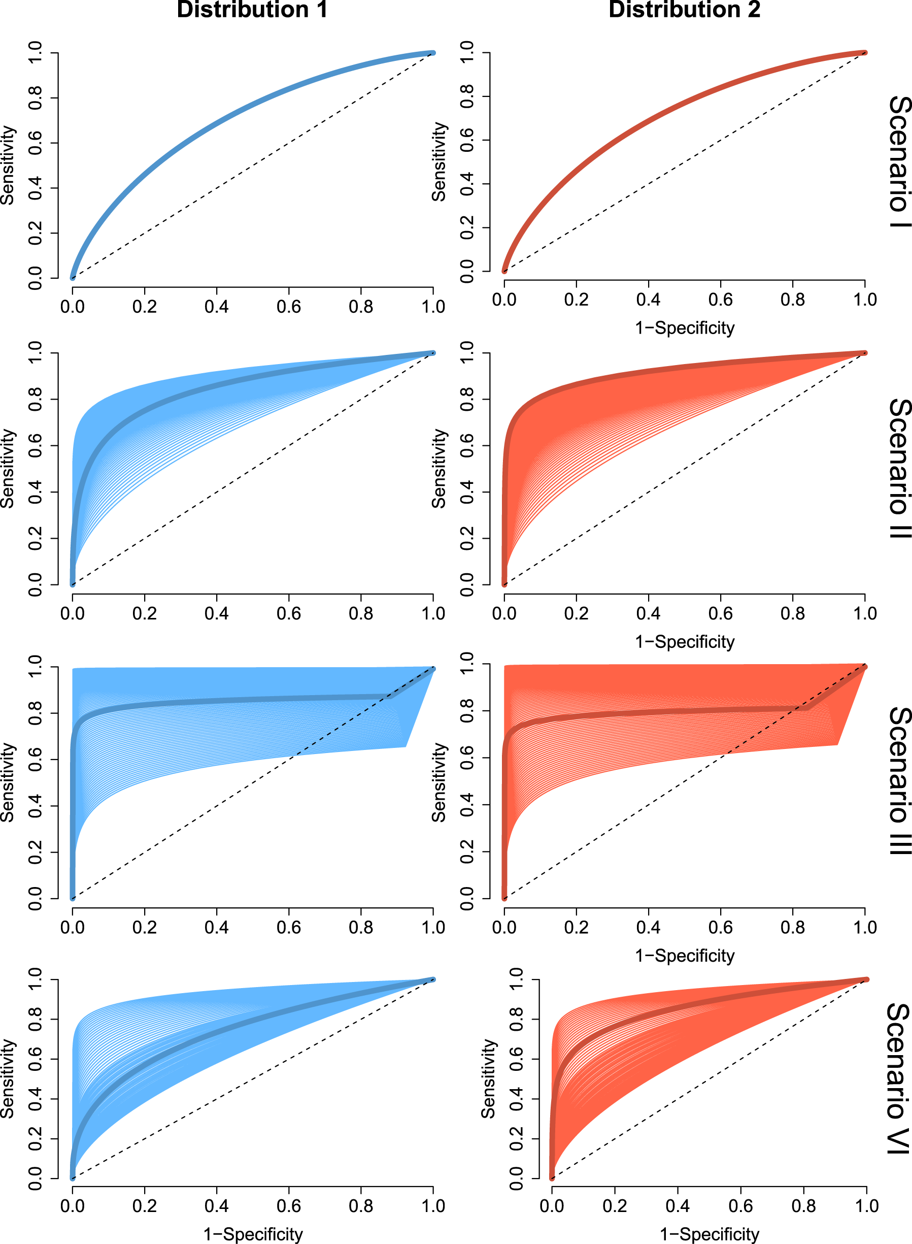
Models I to IV (covariate-specific receiver operating characteristic (ROC) curves). Pooled (thick line) and covariate-specific ROC curves (colored area) for Scenarios I to IV, and the two covariate distributions considered in the Monte Carlo simulations.

Figure 4.

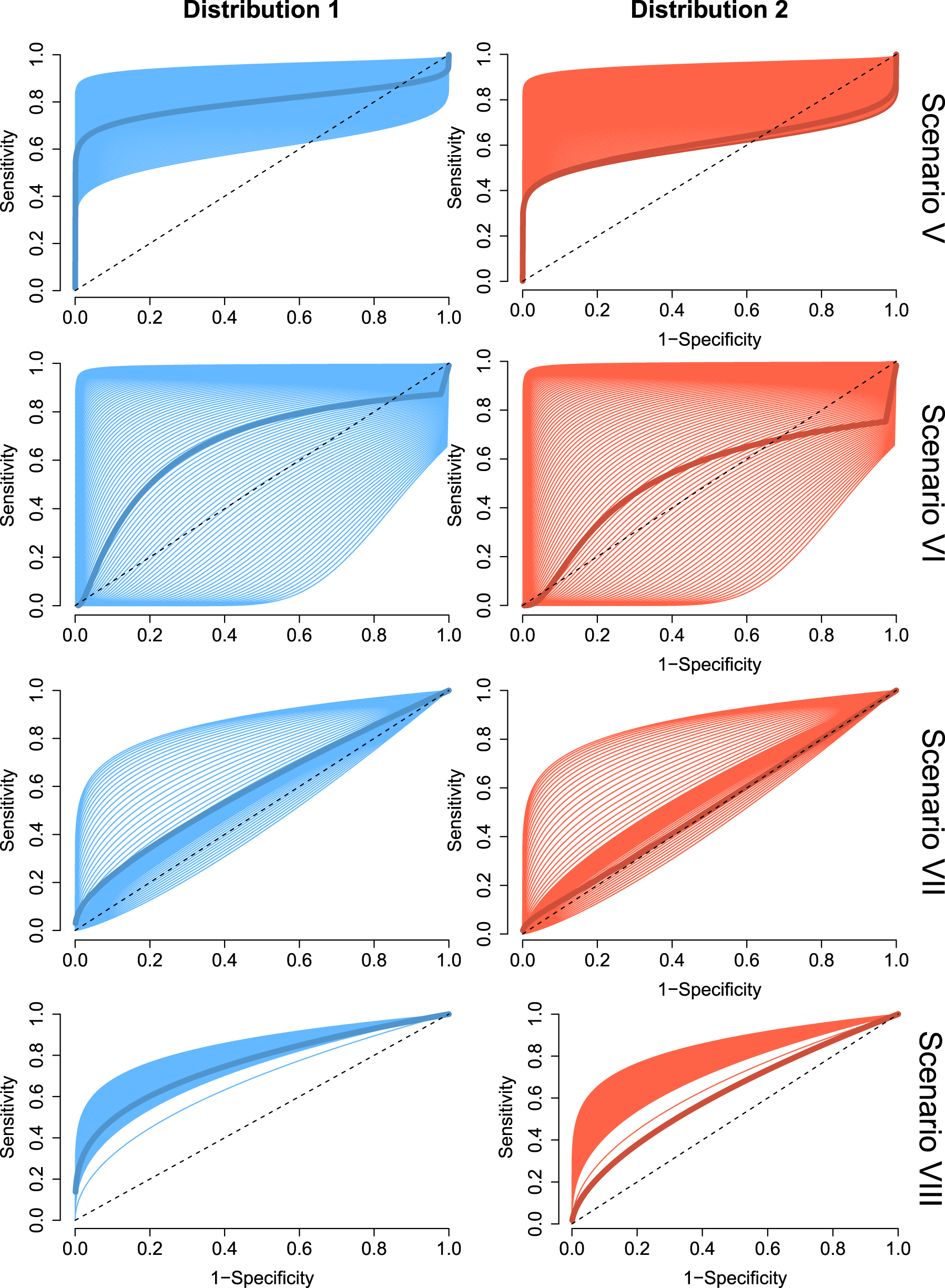
Models V to VIII (covariate-specific receiver operating characteristic (ROC) curves). Pooled (thick line) and covariate-specific ROC curves (colored area) for Scenarios V to VIII, and the two covariate distributions considered in the Monte Carlo simulations.

The first considered configuration for the distribution of the covariate assumes it is uniformly distributed in both the positive and the negative populations, while the second configuration considers Beta distributions with different parameters for the two populations. Particularly,

Distribution 1. $[X | D = 0] \sim U [0, 1]; [X | D = 1] \sim U [0, 1]$

Distribution 2. $[X | D = 0] \sim Beta (1, 1 / 2); [X | D = 1] \sim Beta (1, 2)$

Figures 3 and 4 show the pooled ROC curve for the eight scenarios and the two covariate distributions and the different covariate-specific ROC curves when the covariate takes the values

0.01 \cdot k

(

0 \leq k \leq 100

Remark

In order to gain clarity analyzing Figures 3 and 4, we want to highlight that the pooled (overall) ROC curve is not the average of the covariate-specific ROC curves, but the ROC curve associated with the overall distribution functions.

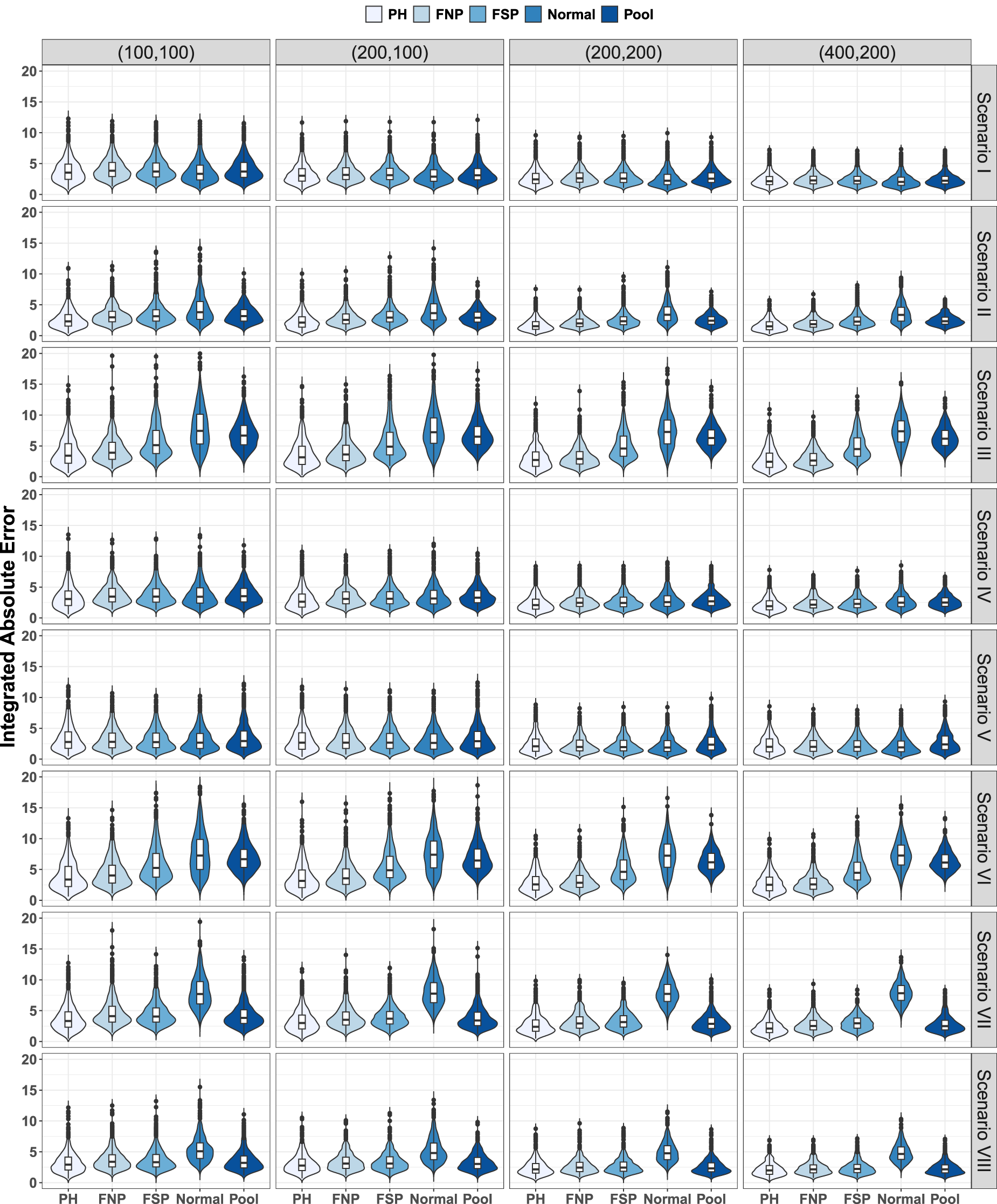
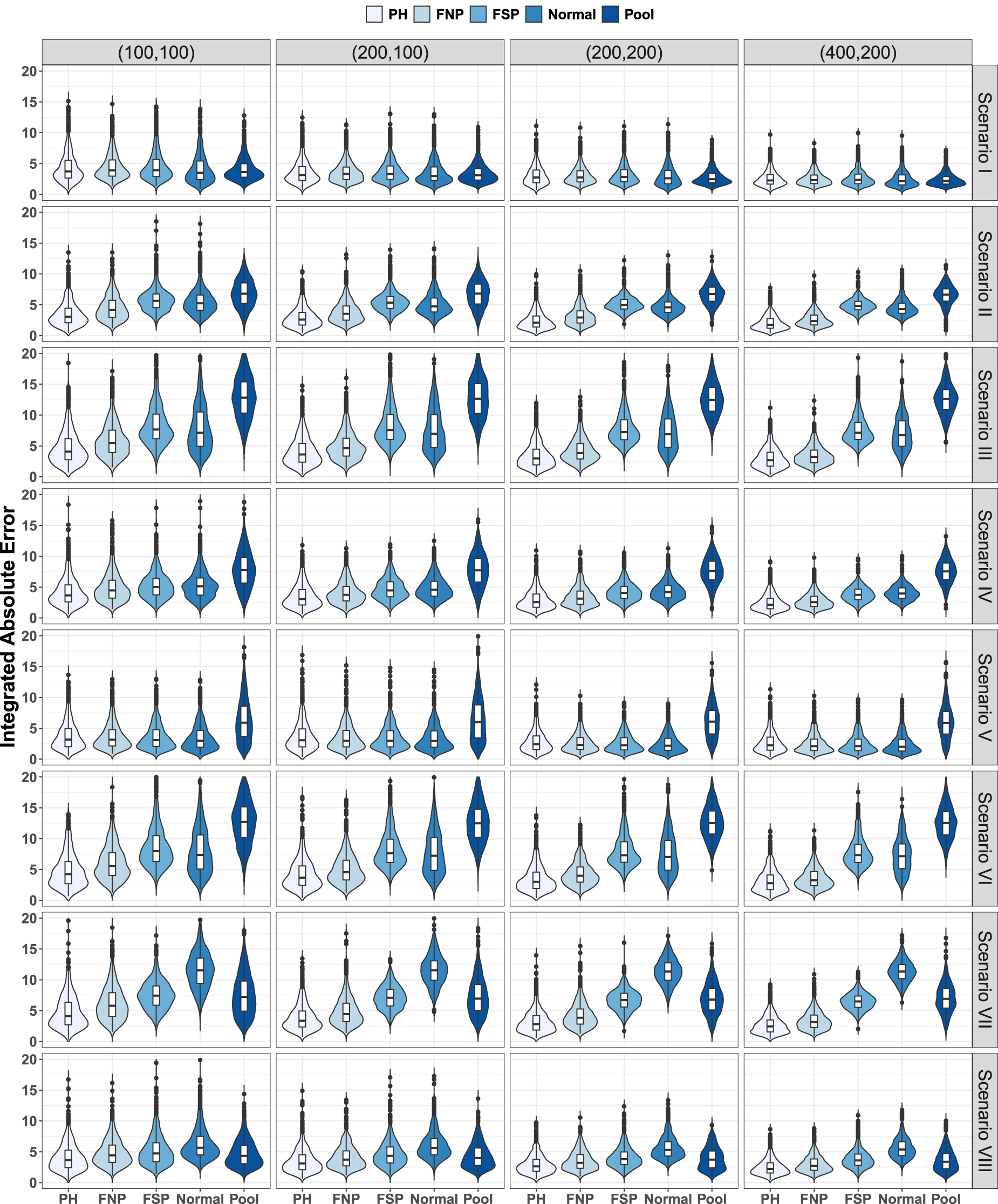
Figures 5 and 6 show the violin plots for the error measure

\int_{R} \int_{0}^{1} | {\hat{R}}_{n} (t | x) - R (t | x) | d t d x \approx \frac{1}{100, 000} \sum_{j = 0}^{100} \sum_{i = 0}^{1000} | {\hat{R}}_{n} (i / 1000 | j / 100) - R ((i / 1000 | j / 100) |

where

{\hat{R}}_{n} (\cdot | x)

and

R (\cdot | x)

are the estimation and the real covariate-specific ROC curves, respectively, based on 1000 Monte Carlo iterations when the covariate follows Distribution 1 (Figure 5) and Distribution 2 (Figure 6). The considered estimators were the proposed PH, the non-parametric induced location-scale regression model considered by González-Manteiga et al.¹⁴ and Rodríguez-Alvarez et al.¹⁵ (FNP), the semi-parametric model proposed by Pepe³² (FSP), the parametric model (assumes normal distributed residuals) proposed by Faraggi¹⁰ (Normal), and the standard pooled non-parametric³³ ROC curve estimator (Pool). FNP, FSP, and Normal estimates were computed using the R package ROCnReg.³⁴ Four different configurations for the sample size were considered:

(n_{0}, n_{1}) = (100, 100), (200, 100), (200, 200)

, and

(400, 200)

Figure 5.

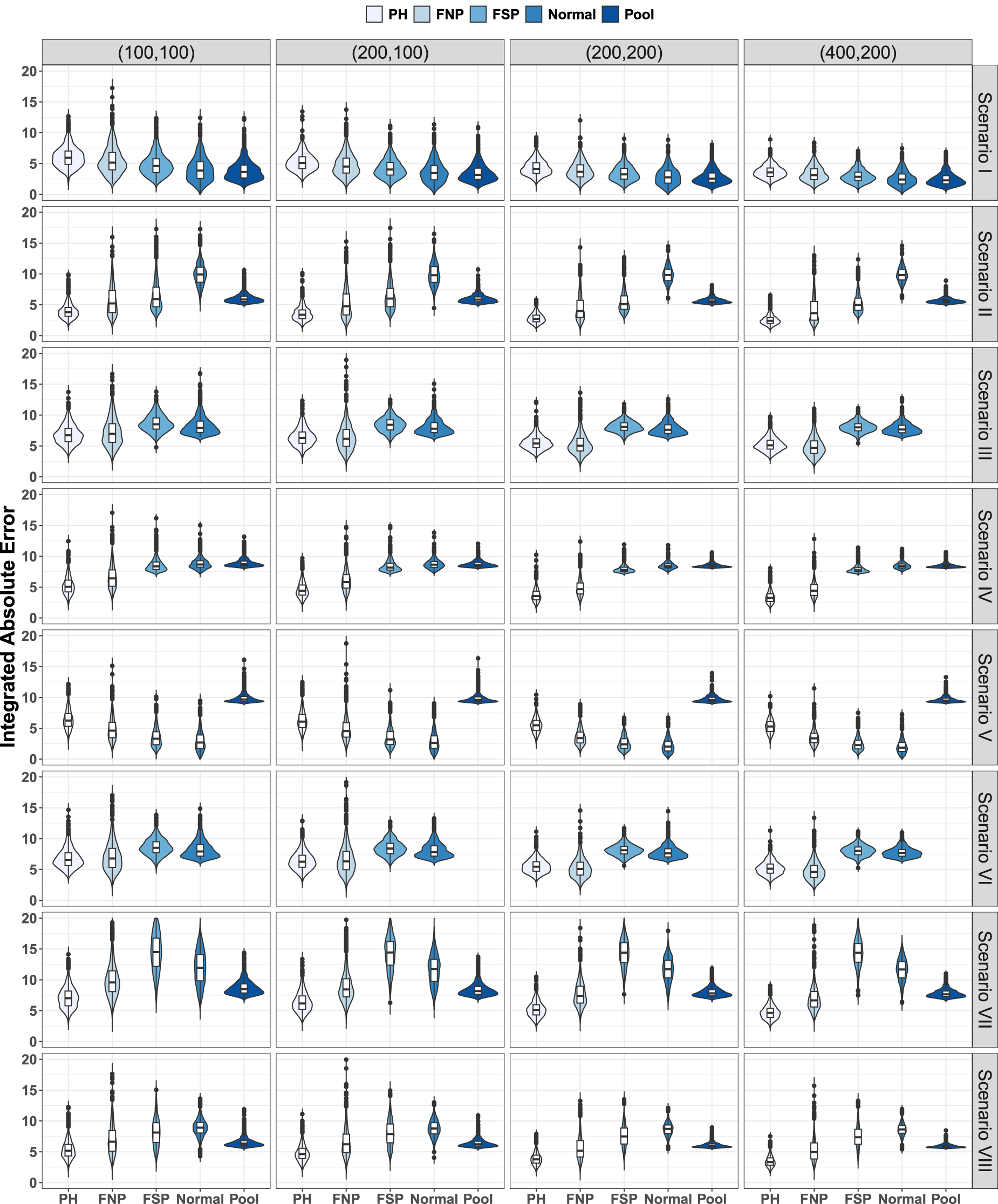
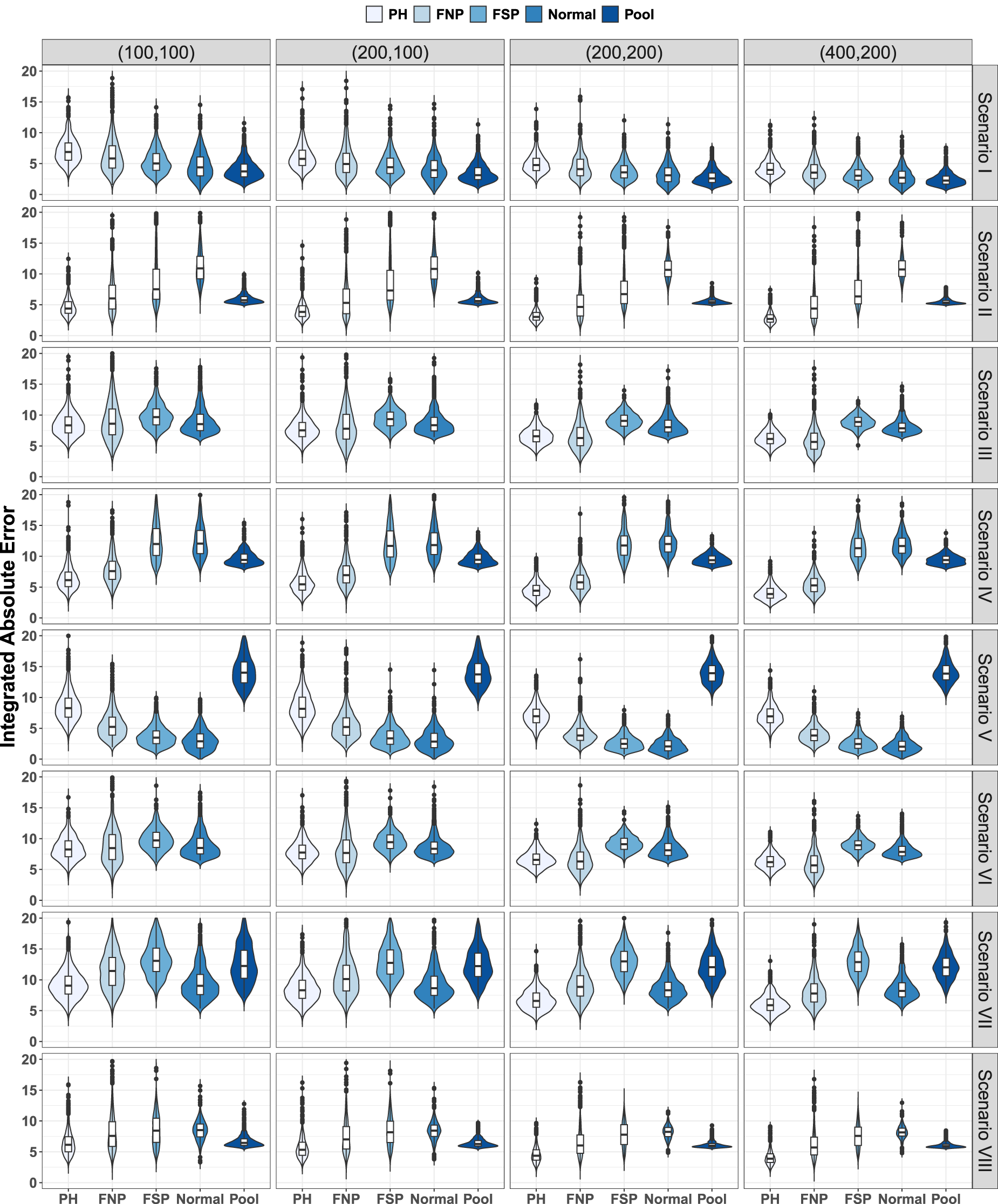
Covariate-specific receiver operating characteristic (ROC) curve. Distribution 1. Violin plots for $\int_{R} \int_{0}^{1} | {\hat{R}}_{n} (t | x) - R (t | x) | d t d x$ , where ${\hat{R}}_{n} (\cdot | x)$ and $R (\cdot | x)$ are the estimation and the real covariate-specific ROC curves, respectively, based on 1000 iterations, for the eight considered scenarios and the four different sample size configurations, $(n_{0}, n_{1})$ . Covariate follows Distribution 1.

Figure 6.

Covariate-specific receiver operating characteristic (ROC) curve. Distribution 2. Violin plots for $\int_{R} \int_{0}^{1} | {\hat{R}}_{n} (t | x) - R (t | x) | d t d x$ , where ${\hat{R}}_{n} (\cdot | x)$ and $R (\cdot | x)$ are the estimation and the real covariate-specific ROC curves, respectively, based on 1000 iterations, for the eight considered scenarios and the four different sample size configurations, $(n_{0}, n_{1})$ . Covariate follows Distribution 2.

Remark

We realize that the used error measure could not be finite for covariates with non bounded dominium. Here, we consider $x \in [0, 1]$ .

Under Distribution 1 (Figure 5), PH and FNP seem to be more affected by noise than FSP and Normal (Scenario I). Under the PH assumption (Scenarios II, IV, VII, and VIII), PH is the clear winner. Spline implementation suffers more with complex functional shapes (Scenarios VII and VIII), although the errors adequately reduce when sample size increases. Despite the pooled estimator (Pool) presents bias in these scenarios, its overall behavior is not worse (even better in some of the configurations) than FSP and Normal. Pool performs better than Normal in Scenario II, and better than FSP and Normal in Scenarios IV and VIII. The behavior of PH and FNP was similar in Scenarios III and VI; FNP was superior to both FSP and Normal. In these two scenarios, the error values for the Pool estimator were out of the considered scale, and the corresponding violin plots are not visible in the figure. Special mention deserves Scenario V. This is probably the most adverse scenario among the considered for the proposed PH estimator; the covariate only impacts on the mean values of the distributions. Since the model is bi-normal and the covariate impact is linear, not surprisingly, FSP and Normal reach the best results. Besides, FNP adapts better than PH to the considered situation, which improves results of Pool, specially, when the sample size increases.

Under Distribution 2 (Figure 6), comparative results among the five considered procedures were similar. However, it is fair to highlight that, in all of them and for the eight considered scenarios and four considered sample size configurations, the level of observed error was much larger than those observed under Distribution 1. Both bias and standard error were much higher for Distribution 2.

We also consider the same eight models, the same two covariate distributions, and the four sample size configurations for studying the behavior of the proposed PH covariate-adjusted ROC curve estimator. Covariate-adjusted versions of the non-parametric induced location-scale regression model (FNP), the Pepe’s frequentist semi-parametric³² (FSP), the Faraggi’s parametric approach¹⁰ (Normal), and the standard pooled non-parametric ROC curve estimators (Pool) are included as reference. R package ROCnReg was used for computing FNP, FSP, and Normal. Figure 7 shows the covariate-adjusted ROC curves for the eight scenarios and the two covariate distributions.

Figure 7.

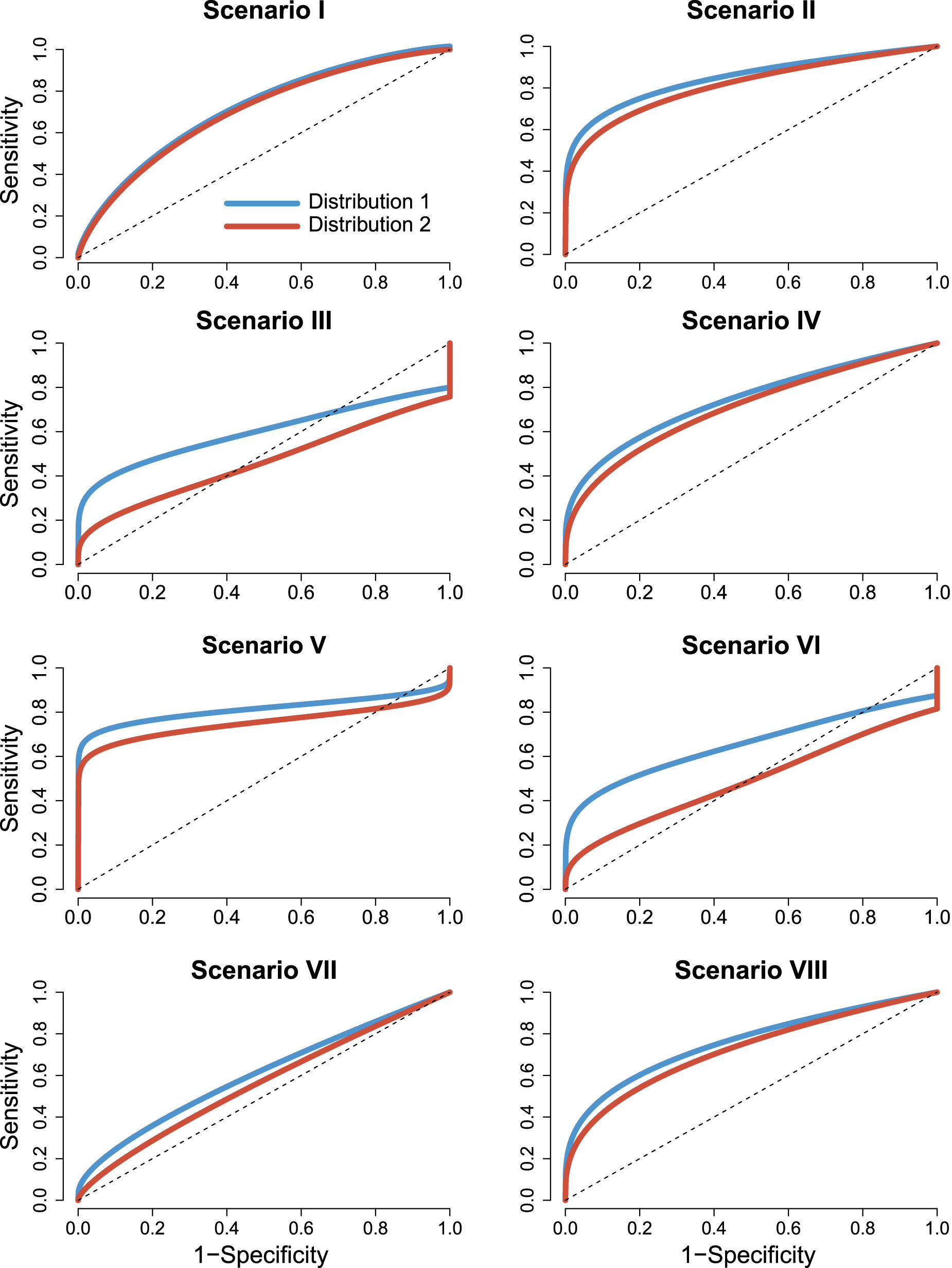
Models (covariate-adjusted receiver operating characteristic (ROC) curves). Covariate-adjusted ROC curves for the eight scenarios considered in the Monte Carlo simulations.

Figures 8 and 9 show the violin plots for the error measure

\int_{0}^{1} | {\hat{a R}}_{n} (t) - a R (t) | d t \approx \frac{1}{100} \sum_{j = 1}^{100} | {\hat{a R}}_{n} (0.01 \cdot j) - a R (0.01 \cdot j) |

where

{\hat{a R}}_{n} (\cdot)

and

a R (\cdot)

are the estimation and the real covariate-adjusted ROC curves, respectively, based on 1000 Monte Carlo iterations, when the covariate follows Distribution 1 and Distribution 2, respectively. Again, the same four configurations for the sample size were considered:

(n_{0}, n_{1}) = (100, 100), (200, 100), (200, 200)

, and

(400, 200)

Figure 8.

Covariate-adjusted receiver operating characteristic (ROC) curve. Distribution 1. Violin plots for $\int_{0}^{1} | {\hat{a R}}_{n} (t) - a R (t) | d t$ , where ${\hat{a R}}_{n} (t)$ and $a R (\cdot | x)$ are the estimation and the real covariate-adjusted ROC curves, respectively, based on 1000 iterations, for the eight considered scenarios and the four sample size configurations, $(n_{0}, n_{1})$ . Covariate follows Distribution 1.

Figure 9.

Covariate-adjusted receiver operating characteristic (ROC) curve. Distribution 2. Violin plots for $\int_{0}^{1} | {\hat{a R}}_{n} (t) - a R (t) | d t$ , where ${\hat{a R}}_{n} (t)$ and $a R (\cdot | x)$ are the estimation and the real covariate-adjusted ROC curves, respectively, based on 1000 iterations, for the eight considered scenarios and the four sample size configurations, $(n_{0}, n_{1})$ . Covariate follows Distribution 2.

In general, the observed differences among the five considered estimators were smaller for the covariate-adjusted than for the covariate-specific ROC curves. Under Distribution 1 (Figure 8), PH obtained clear better results in Scenarios II, III, VI, and VII. FNP was the second classified in Scenarios II, III, and VI. In Scenarios I, IV, and V, the five estimators behave in a very similar way. We can see slightly better results for PH in Scenarios IV and VIII. However, while in Scenario IV, the remaining four estimators behave similarly, in Scenario VIII, Pool was the second classified and Normal clearly obtained the worst results. Highlight that the problems of PH with Scenario V for the covariate-specific ROC curve estimation are diluted for the covariate-adjusted ROC curve. Besides, not surprisingly, Normal procedure did not work on Scenarios VI and VII, and performed poorly in Scenario VIII. Distribution 2 exacerbates, in general, the differences among the estimators and the pooled estimators behaves worse in most of the considered configurations. In Scenario I, the pooled estimator, Pool, was the best, especially for the smallest sample size. In Scenario V, Pool estimator obtained clearly the worst results, while the difference among the remaining four estimators was almost negligible. In Scenarios II, III, IV, VI, VII, and VIII, the proposed PH is again the clear winner, with FNP in the second position. It is worth mentioning that, under Scenarios III, VI, and VIII, PH and FNP clearly outperformed the other three. In Scenarios III and VI, the Pool estimator failed, and part of its errors were out of the considered scale. Finally, we want to highlight the good general performance of FNP, which reached very competitive results in the eight considered scenarios, even in those under the PH assumptions (Scenarios II, IV, VIII, and VIII).

5. Real-world application

For illustrating the practical behavior of the proposed PH estimators in a real-world setting, we consider the synthetic dataset endosyn, publicly available in the R package ROCnReg. The data mimics endocrine data from a cross-sectional study carried out by the Galician Endocrinology and Nutrition Foundation. Detailed information about the original study can be found by Tomé Martínez de Rituerto et al.³⁵

The original study focused in determining the role of the BMI (body mass index) in cardiovascular disease (CVD) risk. With this goal, the 2840 enrolled subjects were classified as positive (691, 24.3%), if they had two or more CVD risk factors (considered risk factors included raised triglycerides, reduced HD-cholesterol, raised blood pressure, and raised fasting plasma glucose), and as negative (2149, 75.7%) otherwise. Here, we want to analyze the capacity of BMI for predicting CVD risk, and also to consider the potential role that demographic factors such as age and gender can play in order to interpret the results. Table 1 describes the variables involved in the study by CVD risk group. Figure 10 contains the directed acyclic graph (DAG)³⁶ showing the potential pathway.

Figure 10.

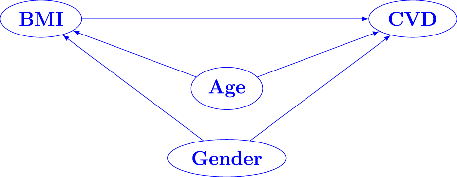
DAG for the endosyn dataset. BMI is affecting CVD, while Age and Gender could affect both BMI and CVD. DAG: directed acyclic graph; BMI: body mass index; CVD: cardiovascular disease.

Table 1.

Descriptive. Basic description for the variables involved in the study by CVD group (with CVD or positive vs. without CVD or negative).

	Total	Positive	Negative
	$n$ = 2840	$n_{1}$ = 691	$n_{0}$ = 2149
BMI, mean $\pm$ sd	26.7 $\pm$ 4.9	29.9 $\pm$ 4.5	25.0 $\pm$ 4.6
Gender (woman), n (%)	1523 (53.6)	273 (39.5)	1250 (58.2)
Age, mean $\pm$ sd	41.4 $\pm$ 15.0	51.5 $\pm$ 15.0	38.2 $\pm$ 13.5

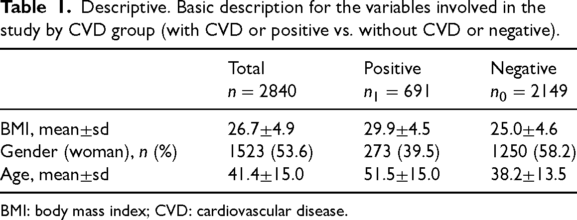
BMI: body mass index; CVD: cardiovascular disease.

The age ranged between 18.3 and 84.7 years old. Individuals in the positive group were, on average, 13.3 years older, had 4.4 kg/m $^{2}$ more BMI, and the percentage of men were 18.7% larger than in the negative group. Besides, there was no relevant difference in the distributions of BMI and age between men and women.

The overall (pooled) AUC, approximated through the empirical estimator, was 0.76 (with a 95% confidence interval based on 5000 bootstrap replications of 0.74–0.78). When we stratified by sex, we have AUCs of 0.72 (0.69–0.75), and 0.80 (0.77–0.83) for men and women, respectively. The covariate-adjusted AUC (aAUC) was, therefore, 0.76 (0.74–0.78). That is, it seems that BMI is more related to CVD in women than in men. Figure 11 (top-left) shows the pooled ROC curve with a 95% confidence band (R package nsROC³⁷ was used in this plot), and covariate-specific (csROC) and covariate-adjusted ROC (aROC) curves by gender (top-right). We checked the GoF of the proposed model through the Grønnesby and Borgan test,²³ which reported p-values of 0.484 and 0.364 in the models associated with the positive and the negative populations in men, respectively, and p-values of 0.244 and 0.318 in the model associated with the positive and the negative populations in women, respectively.

Figure 11.

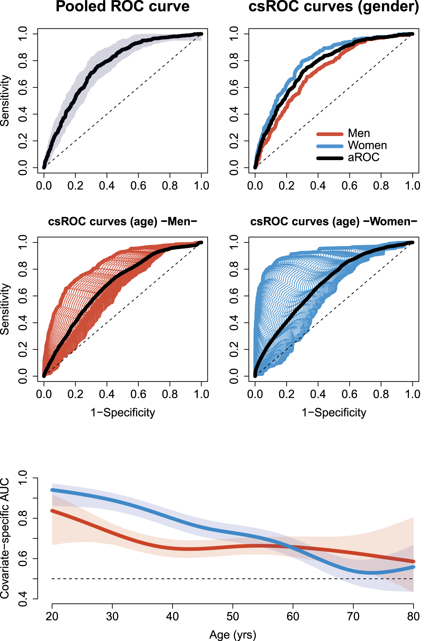
Endosyn data. Pooled ROC curve with 95% confidence bands (top-left). csROC curves by gender and aROC curve (top-right). In the middle, PH csROC curves for different values of ages (ranged between 20 and 80 years old) stratified by gender, and PH aROC curves (in black). Evolution of the csAUC with the age by gender (bottom). ROC: receiver operating characteristic; csROC: covariate-specific receiver operating characteristic; aROC: adjusted receiver operating characteristic; PH: proportional hazard; csAUC: covariate-specific area under the receiver operating characteristic curve.

The PH conditional ROC curves show that age has a great impact on the BMI prediction capacity, specially, in women (Figure 11, middle). In men, the covariate-specific AUCs (csAUCs) oscillated between 0.84 (0.67–0.92) at 20 years, and 0.59 (0.43–0.81) at 80 years; while in women, they oscillated between 0.94 (0.86–0.97) at 20 years, and 0.53 (0.45–0.60) at 73 years (Figure 11, bottom).

6. Conclusions

The so-called “nosological paradigm”³⁸ commonly underlies the statistical approach to the binary classification problem. However, the sensitivity and specificity can be affected for a number of external factors. Thinking about the real pathway between the studied marker, the disease under consideration, and the potential confounders can help to do a better use of the observed results, considering the potential difference between the population used for testing our marker, and the population or subjects particularities on which we are applying our results. This could help us to understand the real accuracy of the marker we are using on a population with particular characteristics, and to customize the threshold we should use in the decision making process. The covariate-specific, or conditional, and the covariate-adjusted ROC curves are valuable tools for addressing the problem. They are based on the conditional distribution functions of the marker on the positive and negative populations. Of course, a variety of estimation procedures have already been proposed in the specialized literature (see Pardo-Fernández et al.¹² for a review of some of these methods).

In this piece of research, we consider the PH Cox regression model for approximating the involved CDFs and, through a direct plug-in procedure, we propose an estimator for the covariate-specific ROC curve. Integrating the resulting estimator with respect to the empirical CDF of the covariate on the positive population provides a PH estimator for the covariate-adjusted ROC curve. In order to gain flexibility in our approximations, a spline procedure is included in the involved Cox regressions.

The huge quantity of papers and books dealing with the theoretical properties of the PH regression models, and other related problems were really helpful in order to develop the asymptotic properties of the estimators here proposed. Although this theory includes both the survival and the hazard functions, being the former more related to our purpose than the latter, we do prefer to present our results in terms of hazard functions, since these function are which actually characterize the problem. Despite theoretically there are no restrictions in order to approximate a multivariate spline function, in practice, dealing with more than one dimension turns the estimation complex, imprecise, and unstable. In these situations, simplifying the problem by using for example additive models would be advisable.

Not surprisingly, Monte Carlo simulations show that the new proposal outperforms its competitors when the underlying model satisfies the required assumptions. The used spline approximation adequately deals with the approximation of non-linear effects. Besides, the PH estimates showed competitive results when some deviations of the original model were introduced. The estimators, however, fail in situations where the impact of the covariate strongly affects the location parameter and does not affect (or affects in an “non controllable” way) the shape of the distributions. We provide results from twelve simulation scenarios (eight in the main article and four in the Supplemental Material).

In the considered real-world problem, we can clearly see how these tools help to have a better understanding of the reality. Both the age and gender strongly affect the capacity of BMI for predicting CVD risk. While the overall AUC was 0.76, it oscillated between 0.94 for women in their 20 s and 0.53 for women in her 70 s. That is, the BMI is a good predictive marker for CVD risk in young women (also in young men; the AUC in this group was 0.84), although it loses its accuracy for women in their 70 s. In this problem, results provided by the PH estimators are slightly smoother than those provided by the Bayesian non-parametric approach³⁹ and presented by Rodríguez-Álvarez and Inácio de Carvalho.³⁴ Remarkable that, based on the GoF tests performed, the model proposed in equation (3) is perfectly compatible with the considered data structure.

In short, the proposed estimators are promising tools for approximating both the conditional and the covariate-adjusted ROC curves, which are helpful in order to understand not only the predictive accuracy of the marker of interest, but also the conditions for extrapolating this accuracy, and the way it should be applied on different populations, for example to decide the threshold to be used depending on the population characteristics. Besides, given the number of studies related with PH Cox regressions, the considered methodology could be easily extended to problems in which the marker has measurement restrictions, for instance, limit of detection. Another advantage is the existence of a number of R packages implementing PH Cox regression models, including routines for spline regression, which facilitates the practical computation of the PH ROC curve estimates. As the Supplemental Material, we provide the R code used in the Monte Carlo simulation study (Section 5), and an additional set of simulations.

Supplemental Material

sj-pdf-1-smm-10.1177_09622802241311458 - Supplemental material for Semiparametric estimator for the covariate-specific receiver operating characteristic curve

Supplemental material, sj-pdf-1-smm-10.1177_09622802241311458 for Semiparametric estimator for the covariate-specific receiver operating characteristic curve by Pablo Martínez-Camblor and Juan Carlos Pardo-Fernández in Statistical Methods in Medical Research

Footnotes

Acknowledgements

The authors are grateful to María Xosé Rodríguez-Álvarez for her helpful insight on the topics considered in this article. They also want to acknowledge to the anonymous reviewers and to the AE for their helpful suggestions.

Declaration of conflicting interests

The author(s) declared no potential conflicts of interest with respect to the research, authorship, and/or publication of this article.

Funding

The author(s) disclosed receipt of the following financial support for the research, authorship, and/or publication of this article: This work was supported from the Grants GRUPIN AYUD/2021/50897 from the Asturies Government and PID2020-118101GB-I00 and PID2023-148811NB-I00 from Agencia Estatal de Investigación (Ministerio de Ciencia, Innovación y Universidades, Spanish Government).

Data availability

Data used are publicly available in the R package ROCnReg (>data(endosyn)).

ORCID iD

Pablo Martínez-Camblor

Supplemental material

Supplemental material for this article is available online. As Supplemental Material, we provide: the R code used in Section 4, and a document containing additional Monte Carlo simulations.

Proofs of the theorems

We want to highlight that, in the proofs of the theorems, we are assuming that parameters of the involved spline function are fixed. This introduces a gap between the considered practical implementation, in which we used penalized splines, and the theoretical results. To consider an adaptative solution for the smooth function could imply to lose the convergence ratio, since the convergence rate of the spline function would not be $n^{1 / 2}$ anymore. Proof of Theorem 1. <i>Proof of Theorem</i> 1.

We are proving the equivalent result

sup_{t \in [0, 1]} | \log {{\hat{R}}_{n} (t | x)} - \log {R (t | x)} | {\overset{P}{⟶}}_{n} 0

From the classical counting processes theory (see, for instance, Chapter 5 by Kalbfleish and Prentice⁴⁰), we know that, for each

x

, and for

d \in {0, 1}

sup_{s \in [0, T]} | {\hat{Λ}}_{d, n_{d}} (s | x) - Λ_{d} (s | x) | {\overset{P}{⟶}}_{n_{d}} 0

with $F_{d} (T) = 1$ . Besides, arguing as by Díaz-Coto et al.,⁴¹ we have that

\begin{aligned} \log {{\hat{R}}_{n} (t | x)} - \log {R (t | x)} = Λ_{1} (Λ_{0}^{- 1} (\log {1 / t} | x) | x) - {\hat{Λ}}_{1, n_{1}} ({\hat{Λ}}_{0, n_{0}}^{- 1} (\log {1 / t} | x) | x) \\ = [Λ_{1} (Λ_{0}^{- 1} (u^{t} | x) | x) - Λ_{1} (Λ_{0}^{- 1} (u_{x, n_{0}}^{t} | x) | x)] + [Λ_{1} (Λ_{0}^{- 1} (u_{x, n_{0}}^{t} | x) | x) - {\hat{Λ}}_{1, n_{1}} ({\hat{Λ}}_{0, n_{0}}^{- 1} (u_{x, m}^{t} | x) | x)] \\ = \frac{λ_{1} (Λ_{0}^{- 1} (u^{t} | x) | x)}{λ_{0} (Λ_{0}^{- 1} (u^{t} | x) | x)} \cdot [{\hat{Λ}}_{0, n_{0}} (s_{x, n_{0}}^{t} | x) - Λ_{0} (s_{x, n_{0}}^{t} | x)] + [Λ_{1} (s_{x, n_{0}}^{t} | x) - {\hat{Λ}}_{1, n_{1}} (s_{x, n_{0}}^{t} | x)] \\ + o_{P} (u^{t} - u_{x, n_{0}}^{t})^{2} \end{aligned}

where

u^{t} = \log {1 / t}

(

= {\hat{Λ}}_{0, n_{0}} (s_{x, n_{0}}^{t} | x)

), and

u_{x, n_{0}}^{t} = Λ_{0} (s_{x, n_{0}}^{t} | x)

, with

s_{x, n_{0}}^{t} = {\hat{Λ}}_{0, n_{0}}^{- 1} (u^{t} | x)

. Therefore, the regularity conditions on the risk functions guarantee the results.

Proof of Theorem 2. <i>Proof of Theorem</i> 2.

Similarly to Lemma 6.1 by Tsiatis,⁴² for $d \in {0, 1}$ , we have that

\begin{aligned} \sqrt{n_{1}} \cdot [{\hat{Λ}}_{0, n_{0}} (s | x) - Λ_{0} (s | x)] {\overset{L}{⟶}}_{n_{1}} ℓ \cdot G_{0} {s, Λ_{0} (∙ | x)} \\ \sqrt{n_{1}} \cdot [{\hat{Λ}}_{1, n_{1}} (s | x) - Λ_{1} (s | x)] {\overset{L}{⟶}}_{n_{1}} G_{1} {s, Λ_{1} (∙ | x)} \end{aligned}

where

G_{0} {s, Λ_{0} (∙ | x)}

and

G_{1} {s, Λ_{1} (∙ | x)}

are independent Gaussian processes with particular (and complex) covariance structure (interested readers are referred to the referenced paper for more information about this covariance function). Hence, the processes

\begin{aligned} \sqrt{n_{1}} \cdot [\log {{\hat{R}}_{n} (t | x)} - \log {R (t | x)}] and \\ ℓ \cdot \frac{λ_{1} (Λ_{0}^{- 1} (u^{t} | x) | x)}{λ_{0} (Λ_{0}^{- 1} (u^{t} | x) | x)} \cdot G_{0} {s_{x, n_{0}}^{t}, Λ_{0} (∙ | x)} + G_{1} {s_{x, n_{0}}^{t}, Λ_{1} (∙ | x)} \end{aligned}

have the same asymptotic distribution. Gaussian processes properties and regularity conditions guarantee that

\begin{aligned} G_{0} {s_{x, n_{0}}^{t}, Λ_{0} (∙ | x)} - G_{0} {u^{t}, Λ_{0} (∙ | x)} {\overset{P}{⟶}}_{n_{0}} 0 \\ G_{1} {s_{x, n_{0}}^{t}, Λ_{1} (∙ | x)} - G_{1} {Λ_{1} (Λ_{0}^{- 1} (u^{t} | x) | x), Λ_{0} (∙ | x)} {\overset{P}{⟶}}_{n_{1}} 0 \end{aligned}

concluding the proof.

References

Lusted

. Signal detectability and medical decision-making. Science 1971; 171: 1217–1219.

Hanley

McNeil

. The meaning and use of the area under a receiver operating characteristic (ROC) curve. Radiology 1982; 143: 29–36.

Faraggi

Reiser

. Estimation of the area under the ROC curve. Stat Med 2002; 21: 3093–3106.

Yala

Lehman

Schuster

, et al. A deep learning mammography-based model for improved breast cancer risk prediction. Radiology 2019; 292: 60–66.

Brentnall

Harkness

Astley

, et al. Mammographic density adds accuracy to both the Tyrer-Cuzick and Gail breast cancer risk models in a prospective UK screening cohort. Breast Cancer Res 2015; 17: 1–9.

Janes

Pepe

. Adjusting for covariates in studies of diagnostic, screening, or prognostic markers: an old concept in a new setting. Am J Epidemiol 2008; 168: 89–97.

Janes

Pepe

. Adjusting for covariate effects on classification accuracy using the covariate-adjusted receiver operating characteristic curve. Biometrika 2009; 96: 371–382.

Pepe

. Three approaches to regression analysis of receiver operating characteristic curves for continuous test results. Biometrics 1998; 54: 124–135.

Pepe

. An interpretation for the ROC curve and inference using GLM procedures. Biometrics 2000; 56: 352–359.

10.

Faraggi

. Adjusting receiver operating characteristic curves and related indices for covariates. J R Stat Soc Ser D (Stat) 2003; 52: 179–192.

11.

López de Ullibarri

Cao

Lado C. Cadarso-Suárez

. Nonparametric estimation of conditional ROC curves: application to discrimination tasks in computerized detection of early breast cancer. Comput Stat Data Anal 2005; 52: 2623–2631.

12.

Pardo-Fernandez

Rodríguez-Álvarez

Van Keilegom

. A review on ROC curves in the presence of covariates. Revstat - Stat J 2014; 12: 21–41.

13.

Rodríguez-Álvarez

Roca-Pardiñas

Cadarso-Suárez

. A new flexible direct ROC regression model: application to the detection of cardiovascular risk factors by anthropometric measures. Comput Stat Data Anal 2011; 55: 3257–3270.

14.

González-Manteiga

Pardo-Fernández

Van Keilegom

. ROC curves in non-parametric location-scale regression models. Scand J Stat 2011; 38: 169–184.

15.

Rodríguez-Álvarez

Roca-Pardiñas

Cadarso-Suárez

. ROC curve and covariates: extending induced methodology to the non-parametric framework. Stat Comput 2011; 21: 483–499.

16.

Inácio de Carvalho

Rodríguez-Álvarez

. Bayesian nonparametric inference for the covariate-adjusted ROC curve. arXiv: https://arxiv.org/abs/1806.00473 2018.

17.

Inácio de Carvalho

Rodríguez-Álvarez

. The covariate-adjusted ROC curve: the concept and its importance, review of inferential methods, and a new Bayesian estimator. Stat Sci 2022; 37: 541–561.

18.

Bianco

Boente

. Addressing robust estimation in covariate-specific ROC curves. Econom Stat (in press) 2023. DOI: 10.1016/j.ecosta.2023.04.001.

19.

Bianco

Boente

González-Manteiga

. Robust consistent estimators for ROC curves with covariates. Electron J Stat 2022; 16: 4133–4161.

20.

Cox

. Regression models and life-tables. J R Stat Soc Ser B (Methodol) 1972; 34: 187–220.

21.

Kalbfleisch

Prentice

. Marginal likelihoods based on Cox’s regression and life model. Biometrika 1973; 60: 267–278.

22.

Lin

Wei

. Goodness-of-fit tests for the general Cox regression model. Stat Sin 1991; 1: 1–17.

23.

Grønnesby

Borgan

. A method for checking regression models in survival analysis based on the risk score. Lifetime Data Anal 1996; 2: 315–328.

24.

Parzen

Lipsitz

. A global goodness-of-fit statistic for Cox regression models. Biometrics 1999; 55: 580–584.

25.

Sleeper

Harrington

. Regression splines in the Cox model with application to covariate effects in liver disease. J Am Stat Assoc 1990; 85: 941–949.

26.

Kooperberg

Stone

Truong

. Hazard regression. J Am Stat Assoc 1995; 90: 78–94.

27.

Truong

Stone

. Asymptotics for hazard regression. University of North Carolina. Institute of Statistics Mimeo Series No 2165. 1996.

28.

Strawderman

Tsiatis

. On the asymptotic properties of a flexible hazard estimator. Ann Stat 1996; 24: 41–63.

29.

Perperoglou

Sauerbrei

Abrahamowicz

, et al. A review of spline function procedures in R. BMC Med Res Methodol 2019; 19: 1–16.

30.

Therneau

. A Package for Survival Analysis in R, 2020.

31.

Yoshida

Naito

. Asymptotics for penalised splines in generalised additive models. J Nonparametr Stat 2014; 26: 269–289.

32.

Pepe

. Three approaches to regression analysis of receiver operating characteristic curves for continuous test results. Biometrics 1998; 54: 124–135.

33.

Hsieh

Turnbull

. Nonparametric and semiparametric estimation of the receiver operating characteristic curve. Ann Stat 1996; 24: 25–40.

34.

Rodríguez-Álvarez

Inácio de Carvalho

. ROCnReg: an R package for receiver operating characteristic curve inference with and without covariates. R J 2021; 13: 525–555.

35.

Tomé Martínez de Rituerto

Botana

Cadarso-Suárez

, et al. Prevalence of metabolic syndrome in galicia (NW Spain) on four alternative definitions and association with insulin resistance. J Endocrinol Invest 2009; 32: 505–511.

36.

Pearl

. Causal diagrams for empirical research. Biometrika 1995; 82: 669–688.

37.

Pérez-Fernández

Martínez-Camblor

Filzmoser

, et al. nsROC: an R package for non-standard ROC curve analysis. R J 2018; 10: 55–77.

38.

Guggenmoos-Holzmann

van Houwelingen

. The (in)validity of sensitivity and specificity. Stat Med 2000; 19: 1783–1792.

39.

Inácio de Carvalho

Jara

Hanson

, et al. Bayesian nonparametric ROC regression modeling. Bayesian Anal 2013; 8: 623–646.

40.

Kalbfleisch

Prentice

. The statistical analysis of failure time data. In: Wiley series in probability and statistics. Hoboken, NJ: Wiley, 2002.

41.

Díaz-Coto

Corral-Blanco

Martínez-Camblor

. Two-stage receiver operating-characteristic curve estimator for cohort studies. Int J Biostat 2021; 17: 117–137.

42.

Tsiatis

. A large sample study of Cox’s regression model. Ann Stat 1981; 9: 93–108.

Supplementary Material

Please find the following supplemental material available below.

For Open Access articles published under a Creative Commons License, all supplemental material carries the same license as the article it is associated with.

For non-Open Access articles published, all supplemental material carries a non-exclusive license, and permission requests for re-use of supplemental material or any part of supplemental material shall be sent directly to the copyright owner as specified in the copyright notice associated with the article.

0.00 MB

8.54 MB