The joint quantile regression modeling of mixed ordinal and continuous responses with its application to an obesity risk data

Abstract

In clinical medical health research, individual measurements sometimes appear as a mixture of ordinal and continuous responses. There are some statistical correlations between response indicators. Regarding the joint modeling of mixed responses, the effect of a set of explanatory variables on the conditional mean of mixed responses is usually studied based on a mean regression model. However, mean regression results tend to underperform for data with non-normal errors and outliers. Quantile regression (QR) offers not only robust estimates but also the ability to analyze the impact of explanatory variables on various quantiles of the response variable. In this paper, we propose a joint QR modeling approach for mixed ordinal and continuous responses and apply it to the analysis of a set of obesity risk data. Firstly, we construct the joint QR model for mixed ordinal and continuous responses based on multivariate asymmetric Laplace distribution and a latent variable model. Secondly, we perform parameter estimation of the model using a Markov chain Monte Carlo algorithm. Finally, Monte Carlo simulation and a set of obesity risk data analysis are used to verify the validity of the proposed model and method.

Keywords

The multivariate asymmetric Laplace distribution joint quantile regression mixed responses Markov chain Monte Carlo algorithm latent variable obesity risk

1. Introduction

In practical applications, measured responses sometimes contain a mixture of discrete and continuous responses. In medical research, for instance, heart rate in patients with cardiovascular disease is a continuous response, while the severity of disease is an ordinal response. In educational assessment, a student’s performance is a continuous response, while their attitude toward learning is an ordinal response. In environmental science, the air quality index is a continuous response, while the pollution level is an ordinal response. In the context of the present research and the set of obesity risk data analyzed in Section 6 of this paper, the measures for individuals include body mass index (BMI) and individual obesity level, where BMI is a continuous response and obesity level is an ordinal categorical response. In the above examples, separate modeling of mixed responses may lose correlation between responses. To ensure reliable statistical inference, the joint modeling approach allows for the consideration of correlation between mixed responses. Joint modeling methods for discrete and continuous mixed responses include the multivariate marginal model, multivariate correlated error model, shared effects model, and Copula method.¹ Joint modeling methods for mixed discrete and continuous responses have received extensive attention from scholars. Catalano² implemented binary modeling of clustered continuous and ordinal categorical outcomes. Gueorguieva and Sanacora³ proposed a joint correlation probit model to analyze ordinal and continuous outcomes of repeated measures. Bahrami et al.⁴ proposed a latent variable model to model both continuous and ordinal correlated mixed responses and to account for missing response variables. Teimourian et al.⁵ proposed a joint model for analysing multivariate mixed ordinal and continuous responses where continuous results may be skewed. Buhule et al.⁶ proposed a Bayesian hierarchical joint modeling approach for analyzing highly unbalanced continuous and ordinal data on disease severity. Ekvall and Molstad⁷ proposed a new method to represent the correlation between mixed continuous and discrete responses using an unstructured covariance matrix. Baghfalaki et al.⁸ introduced a new shared parameter joint model of correlated continuous and binary responses by considering different missing patterns for the two longitudinal results. Ahmadi et al.⁹ presented a transition copula model for longitudinal continuous and binary mixed outcomes with different missing patterns.

The above researches are based on the use of mean regression models to study joint modeling of mixed responses, however, mean regression does not typically give robust estimates for data with skewed distribution and outliers. Quantile regression ( QR), introduced by Koenker and Bassett,¹⁰ offers an alternative approach to mean regression. It allows researchers to study how a set of covariates affects various quantiles of the response variable, providing robust estimation results. Yu and Moyeed¹¹ proposed a Bayesian QR method assuming that the error term obeys an asymmetric Laplace (AL) distribution. Koenker¹² introduced a method for estimating longitudinal data in a QR model. Kozumi and Kobayashi¹³ proposed a Gibbs sampling algorithm to facilitate the implementation of a Bayesian QR method. Tian et al.¹⁴ proposed a linear quantile solution method based on an expectation-maximization (EM) algorithm. To analyze multi-response data, some studies have extended univariate QR to multivariate QR, which allows for the simultaneous modeling of multiple dependent variables at different quantile levels. Waldmann and Kneib¹⁵ proposed a Bayesian bivariate QR method. Petrella and Raponi¹⁶ introduced a likelihood-based approach to jointly estimate marginal conditional quantiles of multiple response variables in a linear regression framework, employing the EM algorithm to estimate the parameters by utilizing a mixed location-scale representation after re-parameterization of the multivariate asymmetric Laplace (MAL) distribution. Tian et al.¹⁷ proposed a Bayesian approach for joint estimation of a multivariate QR model and implemented a Bayesian regularization method with $l_{1 / 2}$ penalty for high-dimensional variable selection and parameter estimation. Merlo et al.¹⁸ proposed a quantile hidden semi-Markov regression for multivariate time series analysis to jointly estimate the multivariate quantiles.

In recent years, scholars have studied joint modeling of mixed responses with QR. Ghasemzadeh et al.¹⁹ proposed a joint modeling method for mixed ordinal and continuous responses based on a random effects model. Ghasemzadeh et al.²⁰ proposed an EM algorithm QR method for jointly modeling discrete and continuous mixed responses based on the Gaussian Copula method. Khazaei et al.²¹ proposed a new semiparametric QR method for joint analysis of mixed responses in a Bayesian framework. However, the above studies are based on univariate quantiles to study the modeling of mixed responses at the same quantile level. Therefore, in this paper, we consider multivariate QR to study the modeling of mixed responses at different quantile levels.

Variable selection is also an important issue in statistical research in mixed responses modeling. The purpose of variable selection is to select the most statistically significant or important variables from a set of covariates to construct the most effective predictive model. Some regularization methods based on penalty functions proposed by scholars are least absolute shrinkage and selection operator (LASSO),²² smoothly clipped absolute deviation,²³ elastic net penalty,²⁴ adaptive LASSO,²⁵ bridge regression,²⁶ minimax concave penalty²⁷ and $l_{1 / 2}$ penalty.²⁸ In recent years, scholars have proposed several methods for variable selection in multiple regression models with mixed types of responses. Rothman et al.²⁹ proposed imposing penalties in multiple response regression analysis to achieve variable selection and estimation of regression coefficients and covariance. Chen et al.³⁰ proposed a Bayesian sparse multiple regression with mixed responses model. Wang et al.³¹ introduced a hybrid multivariate Bayesian sparse variable selection method with a shrinkage prior to jointly analyzing mixed continuous and discrete outcomes in a Bayesian framework.

In this paper, we present and examine a new joint QR modeling approach for mixed ordinal and continuous responses. The rest of this paper is structured as follows: A brief introduction to multivariate QR with the MAL distribution is given in Section 2. In Section 3, we establish the joint QR model for mixed ordinal and continuous responses based on the MAL distribution, and we construct the model’s joint hierarchical likelihood. In Section 4, the Markov chain Monte Carlo (MCMC) algorithm is employed to perform the Bayesian inference of the model. In Section 5, we conduct Monte Carlo simulations, and in Section 6 we apply the proposed method to a set of obesity risk data for analysis. Section 7 provides the discussion and conclusion.

2. Multivariate QR and the MAL distribution

2.1. Conditional quantiles for multi-response regression models

When there are two or more observed response variables, a model must account for the correlation among multiple response variables. Petrella et al.¹⁶ introduced the MAL distribution to jointly model the marginal conditional quantiles of multiple response variables, thus extending the AL distribution with univariate QR model to the multivariate case. We consider the following multivariate linear regression model:

\begin{aligned} Y_{i} = β_{τ} X_{i} + ε_{i}, i = 1, 2, \dots, N \end{aligned}

(2.1)

For each individual,

Y_{i} = (Y_{i 1}, \dots, Y_{i p})^{T}

is the observed

p

-variate continuous response variables,

X_{i}

is a

k \times 1

vector of covariates,

β_{τ} = (β_{τ_{1}}, \dots, β_{τ_{p}})^{T}

is a

p \times k

matrix of unknown QR coefficients with

β_{τ_{j}} = (β_{1 τ_{j}}, \dots β_{k τ_{j}})^{T}

j \in (1, \dots, p)

, and

ε_{i} = (ε_{i 1}, \dots ε_{i p})^{T}

is a

p \times 1

vector of error terms. In QR, it is assumed that the

j

th component of the response

Y_{i}

can be modeled as a function of the

k

covariates in

X_{i}

. Then the joint quantile of the covariate

X_{i}

for multiple response variables

Y_{i}

can be modeled as follows:

\begin{aligned} [\begin{matrix} Q_{τ_{1}} (Y_{i 1} | X_{i}) \\ ⋮ \\ Q_{τ_{p}} (Y_{i p} | X_{i}) \end{matrix}] = β_{τ} X_{i} \end{aligned}

(2.2)

where

Q_{τ_{j}} (Y_{i j} | X_{i})

denotes the quantile function of the response

Y_{i j}

at the quantile level

τ_{j}

given the covariate

X_{i}

. In multivariate QR, the unknown QR parameter matrix

β_{τ}

can be solved by optimizing the following objective function:

\begin{aligned} min \sum_{i = 1}^{N} ρ_{τ} (Y_{i} - β_{τ} X_{i}) = [\begin{matrix} min \sum_{i = 1}^{N} ρ_{τ_{1}} (Y_{i 1} - β_{τ_{1}}^{T} X_{i}) \\ ⋮ \\ min \sum_{i = 1}^{N} ρ_{τ_{p}} (Y_{i p} - β_{τ_{p}}^{T} X_{i}) \end{matrix}] \end{aligned}

(2.3)

where

ρ_{τ} (\cdot)

is a check function for the multivariate quantile,

ρ_{τ} (ε_{i}) = (ρ_{τ_{1}} (ε_{i 1}), \dots, ρ_{τ_{p}} (ε_{i p}))^{T}

. The loss function or check function

ρ_{τ_{j}} (\cdot)

is defined in the same way as the loss or check function for the univariate quantile

ρ_{τ} (u) = u (τ - I_{[u < 0]}) = | u | ((1 - τ) I_{(u < 0)} + τ I_{(u > 0)} (u))

. equation (2.3) shows that each component of the error term

ε_{i}

has a univariate quantile equal to 0 at a fixed quantile level

(τ_{1}, \dots, τ_{p})

2.2. The MAL distribution and hierarchical form

In the multiple linear regression model (2.1), it is assumed that the observed response variable $Y_{i} \sim M A L_{p} (β_{τ} X_{i}, D θ, D Σ D)$ . After re-parameterizing this distribution, the probability density function of the MAL distribution is given by

\begin{aligned} f_{Y_{i}} (y_{i} | β_{τ} X_{i}, D θ, D Σ D) = \frac{2 e x p {(y_{i} - β_{τ} X_{i})^{T} D^{- 1} Σ^{- 1} θ}}{(2 π)^{p / 2} | D Σ D |^{1 / 2}} {(\frac{m}{2 + d})}^{υ / 2} K_{υ} (\sqrt{(2 + d) m}) \end{aligned}

(2.4)

where

β_{τ} X_{i}

is the position parameter vector,

D θ

is the scale (or skewness) parameter,

D = diag (σ_{1}, \dots σ_{p})

, and

σ_{j} > 0

θ = (θ_{1}, \dots, θ_{p})^{T}

with generic elements

θ_{j} = \frac{1 - 2 τ_{j}}{τ_{j} (1 - τ_{j})}

. Additionally,

Σ = Δ Ψ Δ

is a

p \times p

positive definite matrix, where

Ψ

is the correlation matrix and

Δ = diag (δ_{1}, \dots, δ_{p})

δ_{j} = \frac{2}{τ_{j} (1 - τ_{j})}

, for all

j \in (1, 2 \dots, p)

m = (y_{i} - β_{τ} X_{i})^{T} (D Σ D)^{- 1} (y_{i} - β_{τ} X_{i}), d = θ^{T} Σ^{- 1} θ

K_{υ} (\cdot)

denotes the third class of modified Bessel functions with index parameter

υ = (2 - p) / 2

Similar to the AL distribution, to facilitate Bayesian inference in QR, $M A L_{p} (β_{τ} X_{i}, D θ, D Σ D)$ can be expressed as the following position-scaling mixture:

\begin{aligned} Y_{i} = β_{τ} X_{i} + D θ W_{i} + \sqrt{W_{i}} D Σ^{1 / 2} Z_{i} \end{aligned}

(2.5)

where

Z_{i} \sim N_{p} (0_{p}, I_{p})

denotes the

p

-variate standard normal distribution,

W_{i} \sim E x p (1)

denotes the standard exponential distribution, and

Z_{i}

and

W_{i}

are independent of each other.

W_{i}

is the latent variable. Based on the proof presented by Petrella,¹⁶ the marginal distribution of the MAL distribution is

A L (β_{τ_{j}}^{T} X_{i}, σ_{j}, τ_{j})

j \in (1, 2 \dots, p)

. Therefore, based on the mixed location-scale representation of the MAL distribution (2.5), the MAL distribution can be expressed as the following hierarchical structure:

\begin{aligned} Y_{i} | W_{i} \sim N (β_{τ} X_{i} + D θ W_{i}, W_{i} D Σ D), W_{i} \sim E x p (1) \end{aligned}

(2.6)

3. Joint QR model of mixed ordinal and continuous responses

3.1. The proposed model

In this section, we consider our joint regression model for mixed ordinal and continuous responses. The modeling methods for ordinal responses include the probit model, the logit model, and the latent variable model. The probit model and logit model are mainly focused on the conditional mean of ordinal responses, while the latent variable model can model the quantile of ordinal responses. In the following, the joint QR model for the ordinal and continuous mixed responses is constructed based on the latent variable model and the MAL distribution in Section 2.2.

Suppose there are $N$ observations and the observed responses of the $i$ th individual are $(Z_{i}, Y_{2 i})$ , where $Z_{i}$ is the observed ordinal response variable and $Y_{2 i}$ is the observed continuous response variable. For the ordinal response $Z_{i}$ , a latent continuous variable $Y_{1 i}$ is introduced and their relationship is given by

\begin{aligned} Z_{i} = {\begin{cases} 1, α_{0} < Y_{1 i} \leq α_{1}; \\ r, α_{r - 1} < Y_{1 i} \leq α_{r}; \\ R, α_{R - 1} < Y_{1 i} \leq α_{R} \end{cases} \end{aligned}

(3.1)

where cut points

α_{0}, α_{1}, α_{r}, \dots, α_{R}

are strictly incremental thresholds, and

α_{0} = - \infty, α_{R} = \infty

r = 2, \dots R - 1.

In order to jointly model the mixed ordinal and continuous responses and simultaneously account for the correlation between them using model errors, we assume that $Y_{1 i}$ and $Y_{2 i}$ satisfy the following linear regression model

\begin{aligned} {\begin{cases} Y_{1 i} = β_{τ_{1}}^{T} X_{i} + ε_{1 i}; \\ Y_{2 i} = β_{τ_{2}}^{T} X_{i} + ε_{2 i} \end{cases} \end{aligned}

(3.2)

Denote

Y_{i} = (Y_{1 i}, Y_{2 i})^{T}

β_{τ} = (β_{τ_{1}}, β_{τ_{2}})^{T}

is a

2 \times k

regression coefficients matrix,

X_{i}

is a

k \times 1

covariates vector,

ε_{i} = (ε_{1 i}, ε_{2 i})^{T}

is the bivariate error term, equation (3.2) can be written as follows:

\begin{aligned} Y_{i} = β_{τ} X_{i} + ε_{i} \end{aligned}

(3.3)

For the equation (3.3), we assume that

ε_{i} \sim M A L_{2} (0, D θ, D Σ D)

, and therefore

Y_{i} \sim M A L_{2} (β_{τ} X_{i}, D θ, D Σ D)

, where

β_{τ} X_{i}

is the location parameter vector of

Y_{i}

D θ

is the scale (or skewness) parameter,

D = diag (σ_{1}, σ_{2})

σ_{j} > 0

j = 1, 2

;

θ = (θ_{1}, θ_{2})^{T}

θ_{j} = \frac{1 - 2 τ_{j}}{τ_{j} (1 - τ_{j})}

Σ = Δ Ψ Δ

Δ = diag (δ_{1}, δ_{2})

δ_{j} = \frac{2}{τ_{j} (1 - τ_{j})}

. It is the correlation matrix

Ψ

that is the measure of the correlation between the mixed responses. Assuming a hierarchical normal representation based on the location-scale mixture of the MAL distribution,

M A L_{2} (β_{τ} X_{i}, D θ, D Σ D)

can be represented as the following hierarchical structure:

\begin{aligned} Y_{i} = β_{τ} X_{i} + D θ W_{i} + \sqrt{W_{i}} D Σ^{1 / 2} U_{i} \end{aligned}

(3.4)

where

U_{i}

follows a bivariate standard normal distribution, that is,

U_{i} \sim N (0, I_{2})

W_{i} \sim E x p (1)

, and

U_{i}

is independent of

W_{i}

Y_{i} | W_{i} \sim N (β_{τ} X_{i} + D θ W_{i}, W_{i} D Σ D)

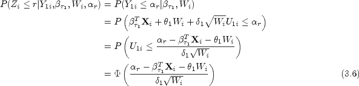
According to the proof of Petrella,¹⁶ the marginal distribution of the MAL distribution is a univariate AL distribution. Then the continuous latent variable associated with the ordinal response $Z_{i}$ is $Y_{1 i} \sim A L (β_{τ_{1}}^{T} X_{i}, σ_{1}, τ_{1})$ . For the purpose of the ordinal model’s identifiability, $σ_{1}$ is set to 1. $Y_{1 i}$ can be represented hierarchically as follows:

\begin{aligned} Y_{1 i} & = β_{τ_{1}}^{T} X_{i} + θ_{1} W_{i} + δ_{1} \sqrt{W_{i}} U_{1 i} \\ = β_{τ_{1}}^{T} X_{i} + \frac{1 - 2 τ_{1}}{τ_{1} (1 - τ_{1})} W_{i} + \sqrt{\frac{2 W_{i}}{τ_{1} (1 - τ_{1})}} U_{1 i} \end{aligned}

(3.5)

where

W_{i} \sim E x p (1)

U_{1 i} \sim N (0, 1)

. Given

W_{i}

Y_{1 i}

follows a normal distribution with mean

β_{τ_{1}}^{T} X_{i}

, variance

{δ_{1}}^{2} W_{i}

, that is,

Y_{1 i} | W_{i} \sim N (β_{τ_{1}}^{T} X_{i}, {δ_{1}}^{2} W_{i})

3.2. Joint hierarchical likelihood

Let $Θ = (β_{τ}, D, Ψ, α)$ is a set of unknown parameters. Let $Y = (Y_{1}, Y_{2})$ . $Z$ and $Y_{2}$ are the observed ordinal and continuous response data, respectively. In model (3.4) and (3.5), $Y_{1 i}$ and $W_{i}$ are the unobserved latent variables. For the ordinal response $Z$ , the cumulative density function (CDF) of the observed response $Z_{i}$ belonging to the $r$ th class is given as

\begin{aligned} P (Z_{i} \leq r | Y_{1 i}, β_{τ_{1}}, W_{i}, α_{r}) & = P (Y_{1 i} \leq α_{r} | β_{τ_{1}}, W_{i}) \\ = P (β_{τ_{1}}^{T} X_{i} + θ_{1} W_{i} + δ_{1} \sqrt{W_{i}} U_{1 i} \leq α_{r}) \\ = P (U_{1 i} \leq \frac{α_{r} - β_{τ_{1}}^{T} X_{i} - θ_{1} W_{i}}{δ_{1} \sqrt{W_{i}}}) \\ = Φ (\frac{α_{r} - β_{τ_{1}}^{T} X_{i} - θ_{1} W_{i}}{δ_{1} \sqrt{W_{i}}}) \end{aligned}

(3.6)

Thus, the probability that the observable response

Z_{i}

belongs to the

r

th class is given as

\begin{aligned} π_{i r} & = P (Z_{i} = r | Y_{1 i}, β_{τ_{1}}, W_{i}, α_{r - 1}, α_{r}) \\ = P (α_{r - 1} < Y_{1 i} \leq α_{r} | β_{τ_{1}}, W_{i}) \\ = Φ (\frac{α_{r} - β_{τ_{1}}^{T} X_{i} - θ_{1} W_{i}}{δ_{1} \sqrt{W_{i}}}) - Φ (\frac{α_{r - 1} - β_{τ_{1}}^{T} X_{i} - θ_{1} W_{i}}{δ_{1} \sqrt{W_{i}}}) \end{aligned}

(3.7)

where

Φ

is the CDF of the standard normal distribution. Therefore, the conditional distribution of

Z

and

Y

can be written as

\begin{aligned} Y_{i} | β_{τ}, D, Ψ, W_{i} \sim N (β_{τ} X_{i} + D θ W_{i}, W_{i} D Σ D); \\ Z_{i} | β_{τ_{1}}, W_{i}, α \sim Multinomial (π_{i 1}, π_{i 2}, \dots, π_{i R}) \end{aligned}

(3.8)

The joint hierarchical likelihood of the complete data for the proposed model can be expressed as follows:

\begin{aligned} L_{C} (Z, Y_{1}, Y_{2}, W | β_{τ}, D, Ψ, α) & = f (Z | β_{τ 1}, α, W) f (Y | β_{τ}, D, Ψ, W) f (W) \\ = \prod_{i = 1}^{N} f (Z_{i} | β_{τ 1}, α, W_{i}) f (Y_{i} | β_{τ}, D, Ψ, W_{i}) f (W_{i}) \\ = \prod_{i = 1}^{N} \prod_{r = 1}^{R} {π_{i r}}^{I (Z_{i} = r)} \times \frac{1}{2 π {| W_{i} D Σ D |}^{1 / 2}} \\ \times \exp {- \frac{1}{2} {(Y_{i} - μ_{i})}^{T} {(W_{i} D Σ D)}^{- 1} (Y_{i} - μ_{i})} \exp {- W_{i}} \end{aligned}

(3.9)

where

μ_{i} = β_{τ} X_{i} + D θ W_{i}

I (\cdot)

is an indicator function of

Z_{i}

that takes the value 1 if the observed response

Z_{i}

belongs to the

r

th class, and 0 otherwise.

4. Bayesian estimation method

4.1. Priors

For unknown parameters, we next consider appropriate prior distributions. The unknown parameters of the proposed model are estimated through posterior inference based on the joint posterior probability density. The Gibbs sampling algorithm is utilized for parameter estimation. The scale parameter $σ_{1} = 1$ in the ordinal part for parameter identifiability, so for consistency and simplicity, we set $σ_{2} = 1$ . In this paper, we consider imposing $l_{1 / 2}$ penalty prior on the proposed joint model. Generalized Gaussian distribution (GGD) is used as prior for the elements of regression coefficients matrix $β_{τ}$ :

\begin{aligned} π (β_{τ}) = \prod_{j = 1}^{2} \prod_{k = 1}^{K} π (β_{τ_{j, k}} | λ_{j, k}), π (β_{j, k} | λ_{j, k}) = \frac{λ_{j, k}^{2}}{2 Γ (3)} \exp {- λ_{j, k} {| β_{j, k} |}^{1 / 2}} \end{aligned}

(4.1)

where

λ_{j, k} > 0

is the tuning parameter.

Since it is difficult to compute this prior analytically to obtain the expected posterior, we use the mixed representation of the GGD which is simple and effective in that we can decompose the prior distribution of $β_{j, k}$ into the following scaled mixture of uniform-gamma distribution:

\begin{aligned} π (β_{j, k} | λ_{j, k}) = \int_{0}^{\infty} π (β_{j, k} | ω_{j, k}) \cdot π (ω_{j, k} | λ_{j, k}) d ω_{j, k} \end{aligned}

(4.2)

where

π (β_{j, k} | ω_{j, k}) = U n i f o r m (- ω_{j, k}^{2}, ω_{j, k}^{2})

, and

π (ω_{j, k} | λ_{j, k}) = G a m m a (3, λ_{j, k}) .

Hence, the hierarchical representation of the prior for $β_{τ}$ is given as $π (β_{τ}) \propto$

$\prod_{j = 1}^{2} \prod_{k = 1}^{K} π (β_{τ_{j, k}} | ω_{j, k}) \cdot π (ω_{j, k} | λ_{j, k}) .$

The prior distribution with respect to $λ$ is $π (λ) = \prod_{j = 1}^{2} \prod_{k = 1}^{K} π (λ_{j, k}) .$

In this paper, when addressing ordinal responses, we assume a zero intercept term for the ordinal model for the purpose of parameter identifiability. We specify the prior distribution of the cut-point threshold $α$ as a truncated normal distribution over the interval $(α_{r - 1}, α_{r + 1})$ , as follows:

\begin{aligned} α_{r} | α_{1}, α_{2}, \dots, α_{r - 1} \sim T N (μ_{α}, σ_{α}, α_{r - 1}, α_{r + 1}) \end{aligned}

(4.3)

where

α = (α_{0}, α_{1}, \dots, α_{R})

r = 1, 2, \dots, R

. Based on

Y_{1 i} | β_{τ_{1}}, W_{i} \sim N (β_{τ_{1}}^{T} X_{i} + θ_{1} W_{i}, δ_{1}^{2} W_{i})

, we can obtain the observation

Z_{i} = r

for the ordinal response if

α_{r - 1} < Y_{1 i} \leq α_{r} .

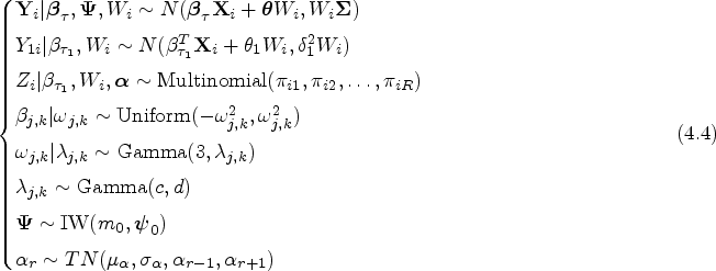
The Bayesian joint hierarchical representation of the joint QR model for mixed ordinal and continuous responses proposed in this paper is given as

\begin{aligned} {\begin{cases} Y_{i} | β_{τ}, Ψ, W_{i} \sim N (β_{τ} X_{i} + θ W_{i}, W_{i} Σ) \\ Y_{1 i} | β_{τ_{1}}, W_{i} \sim N (β_{τ_{1}}^{T} X_{i} + θ_{1} W_{i}, δ_{1}^{2} W_{i}) \\ Z_{i} | β_{τ_{1}}, W_{i}, α \sim Multinomial (π_{i 1}, π_{i 2}, \dots, π_{i R}) \\ β_{j, k} | ω_{j, k} \sim Uniform (- ω_{j, k}^{2}, ω_{j, k}^{2}) \\ ω_{j, k} | λ_{j, k} \sim Gamma (3, λ_{j, k}) \\ λ_{j, k} \sim Gamma (c, d) \\ Ψ \sim IW (m_{0}, ψ_{0}) \\ α_{r} \sim T N (μ_{α}, σ_{α}, α_{r - 1}, α_{r + 1}) \end{cases} \end{aligned}

(4.4)

where the first three lines represent the joint hierarchical likelihood of the model, which includes the distribution of the joint model, the ordinal response and latent variable. The next few lines specify the prior distribution of the unknown parameters.

Therefore, the joint prior for the unknown parameter $β_{τ}, Ψ, α, λ$ is given as

\begin{aligned} π (β_{τ}, Ψ, α, λ) \propto π (β_{τ} | ω) π (ω | λ) π (α) π (Ψ) \end{aligned}

(4.5)

where

ω = {ω_{j, k}}, λ = {λ_{j, k}} .

4.2. Posterior and Gibbs sampling

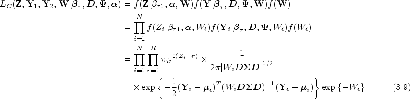
The following joint posterior probability density can be obtained by combining the joint prior and joint likelihood for the specified unknown parameters:

\begin{aligned} π (β_{τ}, Ψ, α, λ, W, Y_{1} | Y_{2}, Z) \\ \propto & L_{C} (Z, Y_{1}, Y_{2}, W | β_{τ}, Ψ, α) \times π (β_{τ}, Ψ, α, λ) \end{aligned}

(4.6)

Obtaining the posterior distribution of parameters from a complex joint posterior distribution usually requires the MCMC method in the Bayesian estimation method as well as some sampling methods, such as the Gibbs sampling algorithm.

π (θ | \cdot)

denotes the fully conditional posterior distribution of

θ

conditional on all the remaining parameters except

θ

The full conditional posterior distribution of the regression coefficient matrix $β_{τ}$ is as follows:

π (β_{τ} | Ψ, λ, W_{i}) \sim N_{2 \times k} (V, B \otimes Σ) \cdot \prod_{j = 1}^{2} \prod_{k = 1}^{K} I (| β_{j, k} | < ω_{j, k}^{2})

where

N_{2 \times k} (V, B \otimes Σ)

is a

p \times k

dimensional matrix normal distribution, which is parameterized by

V

B

Σ

V_{2 \times k} = \sum_{i = 1}^{N} (W_{i}^{- 1} C_{i} X_{i}^{T}) \cdot B

;

B_{k \times k} = (\sum_{i = 1}^{N} W_{i}^{- 1} X_{i} X_{i}^{T})^{- 1}

;

C_{i} = Y_{i} - θ W_{i}

. Hence,

V e c (β_{τ}) \sim N_{2 \times k} (V e c (V), B \otimes Σ) \cdot \prod_{j = 1}^{2} \prod_{k = 1}^{K} I (| β_{j, k} | < ω_{j, k}^{2})

The fully conditional posterior distribution of the latent variable $Y_{1 i}$ is as follows:

Y_{1 i} | β_{τ_{1}}, W_{i}, α \sim T N_{(α_{r - 1}, α_{r})} (β_{τ_{1}}^{T} X_{i} + θ_{1} W_{i}, δ_{1}^{2} W_{i}), Z_{i} = r

The fully conditional posterior distribution of $Ψ$ is as follows:

π (Ψ | β_{τ}, W_{i}) \sim IW (N + m_{0}, Δ^{- 1} \cdot \sum_{i = 1}^{N} (W_{i}^{- 1} η_{i} η_{i}^{T}) \cdot Δ^{- 1} + ψ_{0})

where

η_{i} = Y_{i} - β_{τ} X_{i} - θ W_{i} .

The fully conditional posterior distribution of the latent variable $W_{i}$ is as follows:

π (W_{i} | β_{τ}, Ψ) \sim GIG (0, l_{i}^{T} (Σ)^{- 1} l_{i}, θ^{T} (Σ)^{- 1} θ + 2)

where

l_{i} = Y_{i} - β_{τ} X_{i} .

The unknown parameters can be directly sampled from the corresponding fully conditional posterior distributions by the Gibbs sampling algorithm of the MCMC method. These samples can be utilized to approximate the posterior distributions of parameters. The Appendix provides a detailed derivation of the fully conditional posterior distributions for partial parameters.

5. Simulation studies

5.1. Generated data

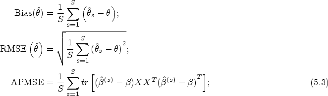
To validate the performance of the joint QR model proposed in Section 3 of this paper, Monte Carlo simulations under several different scenarios are considered in this section. Finally, we also provide an example to illustrate the performance of finite sample for the proposed estimation approach. First, a dataset with a sample size of $N = 150$ was generated. The potential continuous variable associated with the ordinal response $Y_{1 i}$ and continuous response $Y_{2 i}$ were generated by the following linear model:

\begin{aligned} Y_{i} = β X_{i} + ε_{i} \end{aligned}

(5.1)

where

Y_{i} = (Y_{1 i}, Y_{2 i})^{T}

ε_{i} = (ε_{1 i}, ε_{2 i})^{T}

. In model (5.1), the row vectors of the covariates

X_{i}

were generated from the standard normal distribution, respectively. The matrix of regression coefficients

β

was set as

Model 1: $β = (\begin{matrix} - 1 & 1 & 1 \\ 1 & 1 & - 1 \end{matrix}) .$

Model 2: $β = (\begin{matrix} - 1 & 0 & 1 \\ 0 & 1 & 0 \end{matrix}) .$

Model 3: $β = (\begin{matrix} - 1 & 0 & 1 & 0 & 0 & 0 & 0 & 0 & 0 & 0 & 0 & 0 & 0 & 0 & 0 \\ 0 & 1 & - 1 & 0 & 0 & 0 & 0 & 0 & 0 & 0 & 0 & 0 & 0 & 0 & 0 \end{matrix}) .$

where Model 1 represents the dense case, Model 2 the sparse case, and Model 3 very sparse cases. The error terms of model (5.1) were generated from the following two distributions: the errors were generated by (I) a bivariate normal distribution with a mean vector of $0$ and a variance-covariance matrix of $\tilde{Σ}$ . $ε_{i} \sim M N (0, \tilde{Σ})$ , and (II) a bivariate T-distribution with a mean vector $0$ , degree of freedom 3, and scale matrix $\tilde{Σ}$ . $ε_{i} \sim T (3)$ . To consider different correlations between responses by $\tilde{Σ}$ . We selected ${\tilde{Σ}}_{1} = (\begin{matrix} 1 & 0.8 \\ 0.8 & 1 \end{matrix})$ and ${\tilde{Σ}}_{2} = (\begin{matrix} 1 & 0.1 \\ 0.1 & 1 \end{matrix})$ to indicate strong and weak correlation between responses, respectively.

For the ordinal response, we considered four categories in the simulation. The threshold value was taken as $α = c (1, 2, 3)$ . The observation of the ordinal response $Z_{i}$ in (5.1) can take values as follows:

\begin{aligned} Z_{i} = {\begin{cases} 1, 1 \geq Y_{1 i}; \\ 2, 1 < Y_{1 i} \leq 2; \\ 3, 2 < Y_{1 i} \leq 3; \\ 4, 3 < Y_{1 i} \end{cases} \end{aligned}

(5.2)

The hyperparameters of parametric prior distribution were set as

c = 0.1

d = 0.1

. We set

m_{0} = 5 = p + 3

to be a slightly larger value than the data dimension to ensure that the Inverse Wishart distribution is flexible enough to take full account of the diversity of the data without being too centralized or too dispersed, and

ψ_{0} = 0.1 I_{2}

. The settings in simulation with respect to the value of element of correlation matrix

Ψ

were

ρ_{12} = 0.5

and

ρ_{12} = 0.1

. Under different combinations of quantile levels for mixed ordinal and continuous responses,

τ = (0.5, 0.5)

τ = (0.25, 0.75)

, and

τ = (0.75, 0.25)

. The joint QR regression model for mixed-type responses proposed in this paper was fitted to the generated dataset in the Bayesian framework. Simulations were carried out for 100 replications. We ran the Gibbs sampling algorithm for 12,000 iterations, of which the first 3000 iterations were burn-in periods and the remaining were used to perform Bayesian estimation. We evaluated the model performance based on the bias, root mean square error (RMSE), average posteriori mean square error (APMSE) of the regression coefficient estimates, the smaller value of APMSE indicates the better estimation effect of the regression coefficients and coverage rate (CR) for the 95% posterior credible intervals, which are given by

\begin{aligned} Bias (\hat{θ}) & = \frac{1}{S} \sum_{s = 1}^{S} ({\hat{θ}}_{s} - θ); \\ RMSE (\hat{θ}) & = \sqrt{\frac{1}{S} \sum_{s = 1}^{S} {({\hat{θ}}_{s} - θ)}^{2}}; \\ APMSE & = \frac{1}{S} \sum_{s = 1}^{S} t r [({\hat{β}}^{(s)} - β) X X^{T} {({\hat{β}}^{(s)} - β)}^{T}]; \end{aligned}

(5.3)

where

S

is the number of repeated simulations.

{\hat{θ}}_{s}

denotes the estimate of the parameter

θ

for the

s

th simulation.

{\hat{β}}^{(s)}

is the estimate of regression coefficient

β

for the

s

th simulation. All simulations in this paper were implemented using Intel(R) Xeon(R) Gold 6226R CPU @2.90GHz and R 4.3.3 software.

5.2. Convergence diagnostics and model performance analysis

In this simulation, to evaluate the convergence of chains in the Bayesian MCMC algorithm, we ran three MCMC chains with different initial values for 12,000 iterations, of which the first 3,000 iterations were the burn-in period. This simulation was based on Model 1, $ε_{i} \sim M N (0, \tilde{Σ_{1}})$ , quantile level $τ = (0.5, 0.5)$ . Three different initial values were set as follows:

Initial value 1: $β^{(0)} = (\begin{matrix} 1 & 1 & 1 \\ 1 & 1 & 1 \end{matrix})$ , $ρ_{12}^{(0)} = ρ_{21}^{(0)} = 0.3.$

Initial value 2: $β^{(0)} = (\begin{matrix} - 1 & - 1 & - 1 \\ - 1 & - 1 & - 1 \end{matrix})$ , $ρ_{12}^{(0)} = ρ_{21}^{(0)} = 0.5.$

Initial value 3: $β^{(0)} = (\begin{matrix} 1.5 & 1.5 & 1.5 \\ 1.5 & 1.5 & 1.5 \end{matrix})$ , $ρ_{12}^{(0)} = ρ_{21}^{(0)} = 0.7.$

Figure 1 shows three MCMC chains, representing the regression coefficients for different initial values of parameters. This figure shows that as the number of MCMC iterations increases, the posterior sample path diagram of MCMC chains corresponding to the three different initial values shows the characteristics of stabilization, overlapping, and flattening, and the chains fluctuate within a certain interval and remain in a stable range on the whole. Figure 2 displays the autocorrelation plot of the posterior samples of regression coefficients, which exhibit the characteristics of gradually weakening autocorrelation, fluctuation around zero, and disappearance of the trailing effect. These features indicate that the MCMC chain has reached a stable state, and has therefore successfully converged to the target posterior distribution, suggesting that reliable posterior estimation results can be obtained. In order to better illustrate the effect of the Gibbs sampling algorithm, Figure 3 displays the MCMC path plots of regression coefficients, and Figure 4 displays the histogram of posterior sample probability density of the regression parameters for 12,000 iterations. Three MCMC chains of regression coefficients when the parameters take three different sets of initial values. Note: Red lines indicate MCMC chains with initial value 1, blue lines indicate MCMC chains with initial value 2, and black lines indicate MCMC chains with initial value 3.

Figure 1.

Three Markov chain Monte Carlo (MCMC) chains of regression coefficients when the parameters take three different sets of initial values. Note: Red lines indicate MCMC chains with initial value 1, blue lines indicate MCMC chains with initial value 2, and black lines indicate MCMC chains with initial value 3.

Figure 2.

Posterior sample path plots of regression coefficients in Markov chain Monte Carlo (MCMC) posterior samples for 12,000 iterations of Gibbs sampling.

Figure 3.

Autocorrelation plots of regression coefficients in Markov chain Monte Carlo (MCMC) posterior samples for 12,000 iterations of Gibbs sampling.

Figure 4.

Histogram of the probability density of regression coefficients in Markov chain Monte Carlo (MCMC) posterior samples for 12,000 iterations of Gibbs sampling.

Table 1 summarizes the estimation results of the MCMC algorithm based on Model 1 when there is a strong correlation between responses. All the results are based on $S = 100$ repetitions of simulation, which include the real values (Real), posterior mean (Est.), bias, CR and RMSE for the estimates of the parameters at three different combinations of quantile levels. The results show that the regression coefficients estimated by the joint QR model proposed in this paper have small bias and small RMSE. Moreover, the regression coefficient estimates show good CR of the 95% confidence intervals. Parameter estimation effects were similar when the model was fitted to data generated under different error distribution assumptions and at different combinations of quantile levels. The results demonstrate that the joint QR model for mixed-type responses proposed in this paper performs well and robustly. To confirm the appropriateness of fitting the joint QR model to mixed and related responses, we fit a separate QR model to the generated data. As shown in Table 2, at three different combinations of quantile levels, the separate QR model’s estimation of the regression coefficients for the continuous response was similar to that of the joint QR model. The separate QR model’s estimations of the regression coefficients for the ordinal response had a larger bias and RMSE compared to the joint QR model. Estimation of regression coefficients in the joint QR model was better than separate QR. Joint modeling of mixed-type responses takes into account the correlation between responses and therefore improves regression estimation performance.

Table 1.

Model 1 (joint QR) fit to strongly correlated data.

			$τ = (0.5, 0.5)$			$τ = (0.25, 0.75)$			$τ = (0.75, 0.25)$
Error	Par.	Real	Bias	RMSE	CR	Bias	RMSE	CR	Bias	RMSE	CR
MN	$β_{11}$	−1	0.014	0.101	0.980	0.035	0.133	0.980	0.017	0.115	0.980
	$β_{12}$	1	−0.020	0.104	0.960	−0.014	0.137	0.960	−0.007	0.123	0.970
	$β_{13}$	1	−0.020	0.102	0.980	−0.043	0.123	0.960	−0.019	0.112	0.990
	$β_{21}$	1	−0.013	0.103	0.960	−0.034	0.119	0.980	−0.014	0.116	0.980
	$β_{22}$	1	−0.018	0.103	0.970	−0.019	0.107	1.000	0.010	0.110	0.970
	$β_{23}$	−1	0.011	0.093	0.990	0.047	0.122	0.970	0.036	0.119	0.990
	$α_{1}$	1	−0.042	0.124	0.980	−0.209	0.231	0.750	0.130	0.178	0.970
	$α_{2}$	2	0.080	0.154	1.000	−0.019	0.151	0.980	0.227	0.270	0.920
	$α_{3}$	3	0.203	0.267	0.950	0.157	0.438	0.940	0.233	0.273	0.990
T(3)	$β_{11}$	−1	−0.002	0.094	0.990	0.043	0.140	0.990	0.039	0.137	0.970
	$β_{12}$	1	−0.028	0.114	0.960	−0.027	0.134	0.980	−0.012	0.139	0.970
	$β_{13}$	1	−0.025	0.098	0.970	−0.040	0.163	0.970	−0.035	0.138	0.960
	$β_{21}$	1	−0.030	0.109	0.960	−0.066	0.145	0.990	−0.024	0.148	0.990
	$β_{22}$	1	−0.021	0.107	0.990	−0.016	0.147	0.970	−0.029	0.149	0.960
	$β_{23}$	−1	0.016	0.171	0.970	0.037	0.140	0.980	0.062	0.147	0.980
	$α_{1}$	1	−0.073	0.133	0.990	−0.236	0.265	0.770	0.064	0.156	0.980
	$α_{2}$	2	0.010	0.115	1.000	−0.100	0.172	0.970	0.102	0.194	0.980
	$α_{3}$	3	0.097	0.196	0.980	0.094	0.189	0.980	0.061	0.187	1.000

RMSE: root mean square error; CR: coverage rate; QR: quantile regression.

Table 2.

Model 1 (separate QR) fit to strongly correlated data.

			$τ = (0.5, 0.5)$			$τ = (0.25, 0.75)$			$τ = (0.75, 0.25)$
Error	Par.	Real	Bias	RMSE	CR	Bias	RMSE	CR	Bias	RMSE	CR
MN	$β_{11}$	−1	−0.059	0.196	0.990	−0.082	0.186	0.960	−0.054	0.205	0.990
	$β_{12}$	1	0.053	0.168	1.000	0.066	0.187	0.970	0.040	0.205	0.980
	$β_{13}$	1	0.062	0.171	1.000	0.066	0.182	1.000	0.037	0.223	0.970
	$β_{21}$	1	−0.016	0.103	0.930	0.008	0.104	0.950	−0.014	0.086	0.920
	$β_{22}$	1	−0.009	0.100	0.930	0.002	0.092	0.940	0.001	0.112	0.920
	$β_{23}$	−1	0.013	0.103	0.970	−0.014	0.113	0.940	0.000	0.094	0.960
	$α_{1}$	1	0.013	0.182	0.990	0.005	0.182	0.970	−0.018	0.229	0.970
	$α_{2}$	2	0.111	0.252	0.990	0.086	0.255	1.000	0.125	0.283	1.000
	$α_{3}$	3	0.212	0.278	1.000	0.259	0.338	1.000	0.191	0.264	1.000
T(3)	$β_{11}$	−1	−0.039	0.215	0.990	−0.014	0.211	0.980	−0.043	0.258	0.980
	$β_{12}$	1	0.028	0.193	0.990	0.021	0.180	0.990	0.009	0.214	0.990
	$β_{13}$	1	0.022	0.182	0.990	0.049	0.187	0.990	0.015	0.238	0.980
	$β_{21}$	1	−0.007	0.099	0.950	0.030	0.167	0.950	0.004	0.141	0.960
	$β_{22}$	1	−0.015	0.114	0.940	0.008	0.129	0.920	0.000	0.137	0.950
	$β_{23}$	−1	0.010	0.110	0.940	0.019	0.121	0.970	0.001	0.137	0.960
	$α_{1}$	1	0.044	0.214	0.980	0.050	0.213	0.960	−0.090	0.272	0.960
	$α_{2}$	2	0.077	0.251	1.000	0.093	0.265	0.970	0.086	0.311	1.000
	$α_{3}$	3	0.146	0.251	1.000	0.220	0.349	1.000	0.125	0.223	1.000

RMSE: root mean square error; CR: coverage rate; QR: quantile regression.

Table 3.

Model 1 (joint QR) fit to weakly correlated data.

			$τ = (0.5, 0.5)$			$τ = (0.25, 0.75)$			$τ = (0.75, 0.25)$
Error	Par.	Real	Bias	RMSE	CR	Bias	RMSE	CR	Bias	RMSE	CR
MN	$β_{11}$	−1	0.028	0.109	0.950	0.032	0.115	0.990	0.019	0.111	0.970
	$β_{12}$	1	−0.006	0.099	0.980	−0.001	0.105	0.990	−0.038	0.118	0.980
	$β_{13}$	1	0.001	0.111	0.960	0.004	0.106	0.990	−0.016	0.105	0.970
	$β_{21}$	1	−0.012	0.104	0.970	−0.025	0.107	0.970	−0.023	0.127	0.950
	$β_{22}$	1	−0.011	0.102	0.970	−0.018	0.121	0.960	0.001	0.116	0.980
	$β_{23}$	−1	0.009	0.104	0.980	0.024	0.105	0.950	0.010	0.101	0.980
	$α_{1}$	1	−0.030	0.101	1.000	−0.162	0.198	0.920	0.068	0.142	0.980
	$α_{2}$	2	0.063	0.156	0.980	0.010	0.119	0.980	0.136	0.202	0.940
	$α_{3}$	3	0.215	0.277	0.920	0.260	0.311	0.890	0.189	0.261	0.980
T(3)	$β_{11}$	−1	0.013	0.100	0.980	0.020	0.137	0.990	0.010	0.107	1.000
	$β_{12}$	1	−0.018	0.101	0.980	−0.041	0.135	0.940	0.003	0.147	0.960
	$β_{13}$	1	−0.024	0.109	0.960	−0.030	0.137	0.940	−0.015	0.127	1.000
	$β_{21}$	1	−0.028	0.106	0.970	−0.031	0.137	0.960	−0.021	0.135	0.970
	$β_{22}$	1	0.001	0.095	0.990	−0.021	0.127	0.940	−0.023	0.140	0.980
	$β_{23}$	−1	0.006	0.108	0.950	0.031	0.136	0.960	0.017	0.112	0.980
	$α_{1}$	1	−0.058	0.151	0.940	−0.167	0.211	0.880	0.051	0.152	0.980
	$α_{2}$	2	0.030	0.148	1.000	−0.025	0.137	1.000	0.068	0.146	1.000
	$α_{3}$	3	0.141	0.217	0.970	0.193	0.258	0.940	0.062	0.197	0.990

RMSE: root mean square error; CR: coverage rate; QR: quantile regression.

To further validate the performance of the proposed joint QR regression model for mixed responses with different correlations, we considered the weak correlation scenario. The results of parameter estimation for the joint QR model and separate QR model are shown in Tables 3 and 4, respectively. Based on weakly correlated data generated separately under two different error distributions, the regression coefficients estimated by the joint QR model under three different combinations of quantile levels had smaller bias and RMSE than the separate QR model. Compared to the separate QR model, the joint QR model estimates regression coefficients for the ordinal response with smaller bias, which aligns with the findings shown in Tables 1 and 2. These findings indicate that the joint QR model proposed in this paper is applicable to mixed ordinal and continuous responses with different degrees of correlation. Table 5 summarizes the APMSE values of the regression coefficients estimated when fitting the joint QR model and separate QR model to two different degrees of correlation. We can see that the APMSE values of the joint QR model’s regression coefficients estimation are smaller than those of the separate QR model under three different combinations of quantile levels and two assumptions regarding the distribution of error. In addition, the joint QR model performs better under the assumption of the normal error distribution than under the T-distribution, and the model performs better at the quantile level (0.5, 0.5).Taking quantile level (0.5, 0.5) as an example, under two different correlation scenarios, the sample size was increased to $N = 250$ . Table 6 shows the parameter estimation results of the method proposed in this paper. The reported results show that the bias and RMSE of regression parameter estimation decrease with the increase of sample size, thus improving the stability and reliability of estimation. In summary, these results confirm the validity of using the joint QR regression model to analyze mixed-type responses.

Table 4.

Model 1 (separate QR) fit to weakly correlated data.

			$τ = (0.5, 0.5)$			$τ = (0.25, 0.75)$			$τ = (0.75, 0.25)$
Error	Par.	Real	Bias	RMSE	CR	Bias	RMSE	CR	Bias	RMSE	CR
MN	$β_{11}$	−1	−0.031	0.187	0.990	−0.087	0.207	0.950	−0.048	0.184	0.980
	$β_{12}$	1	0.025	0.173	1.000	0.096	0.201	0.970	0.036	0.220	1.000
	$β_{13}$	1	0.025	0.162	0.990	0.093	0.205	0.970	0.025	0.204	1.000
	$β_{21}$	1	0.008	0.103	0.970	0.009	0.118	0.930	−0.010	0.098	0.950
	$β_{22}$	1	0.005	0.099	0.910	0.010	0.101	0.960	0.016	0.110	0.940
	$β_{23}$	−1	−0.004	0.101	0.880	0.020	0.112	0.940	−0.010	0.113	0.940
	$α_{1}$	1	0.033	0.200	0.980	0.023	0.174	0.990	−0.025	0.231	0.980
	$α_{2}$	2	0.101	0.271	1.000	0.134	0.255	0.990	0.114	0.303	1.000
	$α_{3}$	3	0.168	0.296	1.000	0.297	0.367	1.000	0.209	0.263	1.000
T(3)	$β_{11}$	−1	−0.018	0.220	0.970	−0.055	0.224	0.980	−0.040	0.259	0.980
	$β_{12}$	1	0.020	0.195	0.970	0.048	0.231	0.970	0.053	0.252	0.970
	$β_{13}$	1	0.025	0.202	0.970	0.022	0.196	1.000	0.011	0.257	0.970
	$β_{21}$	1	−0.005	0.107	0.920	−0.004	0.145	0.940	−0.003	0.146	0.950
	$β_{22}$	1	0.000	0.118	0.970	0.012	0.140	0.920	0.010	0.128	0.970
	$β_{23}$	−1	−0.012	0.111	0.970	−0.004	0.123	0.970	−0.015	0.123	0.960
	$α_{1}$	1	0.038	0.205	0.970	0.022	0.202	0.970	−0.122	0.265	0.950
	$α_{2}$	2	0.061	0.269	1.000	0.105	0.263	0.990	0.072	0.286	1.000
	$α_{3}$	3	0.123	0.267	1.000	0.222	0.345	1.000	0.104	0.215	1.000

RMSE: root mean square error; CR: coverage rate; QR: quantile regression.

Table 5.

APMSE for the estimation of regression coefficients for joint QR and separate QR models.

Response correlation	Model	Error	$τ = (0.5, 0.5)$	$τ = (0.25, 0.75)$	$τ = (0.75, 0.25)$
Strong correlation	Joint QR	MN	8.874	13.387	11.777
		T(3)	9.711	19.340	17.829
	Separate QR	MN	18.766	20.113	23.584
		T(3)	22.584	25.811	33.612
Weak correlation	Joint QR	MN	9.472	10.743	11.050
		T(3)	9.169	15.654	14.400
	Separate QR	MN	17.887	23.592	21.707
		T(3)	24.661	28.689	40.756

APMSE: average posteriori mean square error; QR: quantile regression.

Table 6.

Parameter estimation results with sample size $N = 250$ .

			Strong correlation			Weak correlation
Error	Par.	Real	Bias	RMSE	CR	Bias	RMSE	CR
MN	$β_{11}$	−1	−0.002	0.077	0.980	0.026	0.078	0.980
	$β_{12}$	1	−0.002	0.077	0.960	−0.006	0.070	0.980
	$β_{13}$	1	−0.013	0.089	0.960	0.005	0.085	0.940
	$β_{21}$	1	−0.022	0.080	0.960	−0.004	0.078	0.980
	$β_{22}$	1	−0.002	0.075	0.960	−0.001	0.081	0.980
	$β_{23}$	−1	−0.003	0.088	0.930	0.018	0.075	0.980
	$α_{1}$	1	−0.023	0.091	0.990	−0.018	0.087	1.000
	$α_{2}$	2	0.130	0.166	0.930	0.123	0.169	0.980
	$α_{3}$	3	0.300	0.327	0.810	0.290	0.329	0.720
T(3)	$β_{11}$	−1	−0.002	0.070	0.980	0.009	0.084	0.950
	$β_{12}$	1	0.003	0.080	0.960	−0.015	0.084	0.990
	$β_{13}$	1	−0.002	0.070	1.000	−0.014	0.091	0.950
	$β_{21}$	1	−0.018	0.079	0.970	−0.030	0.094	0.920
	$β_{22}$	1	−0.014	0.080	0.960	−0.007	0.081	0.960
	$β_{23}$	−1	0.011	0.078	0.970	−0.002	0.086	0.990
	$α_{1}$	1	−0.022	0.099	0.980	−0.023	0.094	0.970
	$α_{2}$	2	0.085	0.138	0.970	0.061	0.118	0.980
	$α_{3}$	3	0.186	0.246	0.900	0.205	0.262	0.890

RMSE: root mean square error; CR: coverage rate.

Table 7.

Parameter estimation results of model 2.

			$τ = (0.5, 0.5)$			$τ = (0.25, 0.75)$			$τ = (0.75, 0.25)$
Error	Par.	Real	Bias	RMSE	CR	Bias	RMSE	CR	Bias	RMSE	CR
MN	$β_{11}$	−1	0.012	0.110	0.950	0.013	0.134	0.950	0.014	0.113	1.000
	$β_{12}$	0	0.001	0.051	1.000	−0.001	0.069	0.990	−0.002	0.060	1.000
	$β_{13}$	1	−0.012	0.102	0.980	−0.025	0.140	0.990	−0.031	0.135	0.960
	$β_{21}$	0	0.007	0.063	0.990	−0.001	0.057	1.000	−0.009	0.050	1.000
	$β_{22}$	1	−0.028	0.099	0.990	−0.026	0.138	0.960	−0.038	0.117	0.980
	$β_{23}$	0	−0.013	0.053	1.000	0.004	0.066	1.000	0.014	0.058	1.000
	$α_{1}$	1	−0.009	0.116	0.980	−0.217	0.258	0.730	0.152	0.196	0.930
	$α_{2}$	2	0.124	0.190	0.970	0.025	0.138	0.990	0.299	0.335	0.850
	$α_{3}$	3	0.251	0.305	0.940	0.320	0.361	0.810	0.252	0.306	0.990
T(3)	$β_{11}$	−1	0.020	0.108	0.960	0.059	0.163	0.960	0.045	0.174	0.950
	$β_{12}$	0	0.002	0.071	0.980	0.002	0.074	1.000	0.007	0.064	1.000
	$β_{13}$	1	−0.019	0.115	0.970	−0.050	0.150	0.960	0.003	0.162	0.970
	$β_{21}$	0	0.005	0.054	1.000	−0.003	0.080	1.000	−0.012	0.079	1.000
	$β_{22}$	1	−0.005	0.111	0.950	−0.037	0.164	0.970	−0.069	0.158	0.940
	$β_{23}$	0	−0.007	0.066	1.000	0.008	0.077	1.000	0.012	0.069	1.000
	$α_{1}$	1	−0.040	0.118	0.980	−0.211	0.259	0.770	0.118	0.186	0.950
	$α_{2}$	2	0.057	0.142	1.000	−0.065	0.141	1.000	0.115	0.187	0.990
	$α_{3}$	3	0.149	0.224	0.990	0.184	0.254	0.970	0.075	0.224	1.000

RMSE: root mean square error; CR: coverage rate.

5.3. Variable selection

In this simulation, based on sparse Model 2 and Model 3, we evaluated the performance of the joint model and method proposed in this paper based on both parameter estimation effects and capacity for variable selection. The other simulation settings were the same as those described in Section 5.1. The ability of the model to select sparse variables was assessed in terms of correctly identifying number of significant variables on average (NC) and incorrectly identifying the number of insignificant variables on average (NIC). The results of the parameter estimation and variable selection for the two sparse models are shown in Tables 7 – 9 The results of parameter estimation under different error assumptions and three quantile level combinations include the posterior mean (Est.), bias, CR and RMSE of the parameters. The results of variable selection include NC, NIC, and the number of correct identifications for each regression coefficient in 100 replicate simulations. Tables 7 and 8 show that parameters estimated by both sparse Model 2 and sparse Model 3 exhibited relatively small bias and RMSE, good CR, and with no obvious difference between estimates under different error assumptions. Table 9 shows that in the two sparse model scenarios, the joint QR model proposed in this paper was able to correctly identify all non-zero coefficients. The NIC value of sparse Model 2 was smaller than that of sparse Model 3. The results of variable selection under normal error assumption were better than those of the T-distribution, which is manifested in the fact that, the two sparse models at the levels of three different quantile combinations had smaller NIC values when normal error was assumed. Thus, the study demonstrated that the Bayesian regularization method with $l_{1 / 2}$ penalty achieved better parameter estimation and variable selection ability.

Table 8.
Parameter estimation results of model 3.

$τ = (0.5, 0.5)$ $τ = (0.25, 0.75)$ $τ = (0.75, 0.25)$

Error Par. Real Bias RMSE CR Bias RMSE CR Bias RMSE CR

MN $β_{11}$ −1 0.022 0.103 0.990 0.030 0.116 1.000 0.017 0.114 1.000

$β_{12}$ 0 0.001 0.049 1.000 0.006 0.043 1.000 0.005 0.049 1.000

$β_{13}$ 1 −0.035 0.091 0.990 −0.009 0.101 0.990 −0.029 0.103 0.990

$β_{21}$ 0 0.004 0.044 1.000 −0.002 0.055 1.000 −0.008 0.047 1.000

$β_{22}$ 1 −0.010 0.103 0.960 −0.011 0.113 0.990 −0.016 0.103 0.990

$β_{23}$ −1 0.021 0.095 0.990 0.028 0.106 0.990 0.027 0.102 1.000

$α_{1}$ 1 −0.004 0.110 0.990 −0.203 0.231 0.780 0.184 0.218 0.900

$α_{2}$ 2 0.120 0.174 0.950 0.015 0.125 1.000 0.297 0.328 0.860

$α_{3}$ 3 0.296 0.346 0.890 0.305 0.342 0.820 0.282 0.326 1.000

T(3) $β_{11}$ −1 0.017 0.121 0.970 0.051 0.146 0.960 0.049 0.149 0.950

$β_{12}$ 0 0.002 0.059 1.000 −0.004 0.056 1.000 0.002 0.064 1.000

$β_{13}$ 1 −0.011 0.117 0.970 −0.049 0.144 0.980 −0.042 0.154 0.970

$β_{21}$ 0 0.001 0.055 1.000 0.016 0.054 1.000 0.006 0.066 1.000

$β_{22}$ −1 −0.029 0.113 0.990 −0.042 0.135 0.980 −0.016 0.137 0.980

$β_{23}$ 0 0.019 0.118 0.980 0.026 0.150 0.970 0.025 0.126 0.990

$α_{1}$ 1 −0.024 0.105 1.000 −0.201 0.231 0.810 0.146 0.193 0.940

$α_{2}$ 2 0.060 0.143 1.000 −0.017 0.144 0.980 0.141 0.214 0.970

$α_{3}$ 3 0.141 0.261 0.970 0.218 0.291 0.930 0.044 0.191 1.000

			$τ = (0.5, 0.5)$	$τ = (0.25, 0.75)$	$τ = (0.75, 0.25)$
MN	$β_{11}$	−1	0.022	0.103	0.990	0.030	0.116	1.000	0.017	0.114	1.000
	$β_{12}$	0	0.001	0.049	1.000	0.006	0.043	1.000	0.005	0.049	1.000
	$β_{13}$	1	−0.035	0.091	0.990	−0.009	0.101	0.990	−0.029	0.103	0.990
	$β_{21}$	0	0.004	0.044	1.000	−0.002	0.055	1.000	−0.008	0.047	1.000
	$β_{22}$	1	−0.010	0.103	0.960	−0.011	0.113	0.990	−0.016	0.103	0.990
	$β_{23}$	−1	0.021	0.095	0.990	0.028	0.106	0.990	0.027	0.102	1.000
	$α_{1}$	1	−0.004	0.110	0.990	−0.203	0.231	0.780	0.184	0.218	0.900
	$α_{2}$	2	0.120	0.174	0.950	0.015	0.125	1.000	0.297	0.328	0.860
	$α_{3}$	3	0.296	0.346	0.890	0.305	0.342	0.820	0.282	0.326	1.000
T(3)	$β_{11}$	−1	0.017	0.121	0.970	0.051	0.146	0.960	0.049	0.149	0.950
	$β_{12}$	0	0.002	0.059	1.000	−0.004	0.056	1.000	0.002	0.064	1.000
	$β_{13}$	1	−0.011	0.117	0.970	−0.049	0.144	0.980	−0.042	0.154	0.970
	$β_{21}$	0	0.001	0.055	1.000	0.016	0.054	1.000	0.006	0.066	1.000
	$β_{22}$	−1	−0.029	0.113	0.990	−0.042	0.135	0.980	−0.016	0.137	0.980
	$β_{23}$	0	0.019	0.118	0.980	0.026	0.150	0.970	0.025	0.126	0.990
	$α_{1}$	1	−0.024	0.105	1.000	−0.201	0.231	0.810	0.146	0.193	0.940
	$α_{2}$	2	0.060	0.143	1.000	−0.017	0.144	0.980	0.141	0.214	0.970
	$α_{3}$	3	0.141	0.261	0.970	0.218	0.291	0.930	0.044	0.191	1.000

RMSE: root mean square error; CR: coverage rate.

Table 9.

Variable selection for model 2 and model 3.

Model	$τ$	Error	NC	NIC	$β_{11}$	$β_{12}$	$β_{13}$	$β_{21}$	$β_{22}$	$β_{23}$
Model 2	(0.5,0.5)	MN	3	0.19	100	95	100	91	100	95
		T(3)	3	0.33	100	88	100	92	100	87
	(0.25,0.75)	MN	3	0.29	100	85	100	95	100	91
		T(3)	3	0.42	100	89	100	84	100	85
	(0.75,0.25)	MN	3	0.27	100	89	100	93	100	91
		T(3)	3	0.40	100	89	100	86	100	85
Model 3	(0.5,0.5)	MN	4	1.17	100	94	100	98	100	100
		T(3)	4	1.86	100	90	100	91	100	100
	(0.25,0.75)	MN	4	1.59	100	99	100	91	100	100
		T(3)	4	2.99	100	95	100	94	100	100
	(0.75,0.25)	MN	4	1.82	100	96	100	95	100	100
		T(3)	4	3.01	100	88	100	87	100	100

Table 10.

Description of variables in the obesity risk dataset.

Variable symbol	Variable name	Variable description
$Z$	$o b e$	Obesity level
$Y_{2}$	$b o d y m a s s i n d e x (B M I)$	Body mass index
$X_{1}$	$g e n d e r$	Sex ( $male = 1$ , $female = 0$ )
$X_{2}$	$a g e$	Age
$X_{3}$	$f a m i l y$	Family history of obesity ( $yes = 1$ , $no = 0$ )
$X_{4}$	$f a v c$	Frequent consumption of high calorie foods ( $Yes = 1$ , $No = 0$ )
$X_{5}$	$f c v c$	Frequency of consumption of vegetables
$X_{6}$	$n c p$	Frequency of main meals
$X_{7}$	$c h_{2} o$	Daily water consumption
$X_{8}$	$f a f$	Frequency of exercise

6. Analysis of obesity risk data

This section applies the proposed joint QR model to the analysis of a set of obesity risk data. The dataset was obtained from the Kaggle platform, and the dataset source link is https://www.kaggle.com/datasets/jpkochar/obesity-risk-dataset. The individual information included gender, age, height, weight, family history of overweight, dietary habits, physical activity, and corresponding obesity level. A description of the variables in this dataset is presented in Table 10. The causes of obesity are complex and various, including both the influence of individual lifestyle, and the constraints of environmental and social factors. Individual dietary structure and exercise habits largely determine an individual’s risk of obesity. Elevated levels of obesity can lead to serious health risks. Obesity risk analysis can help people recognize their level of obesity and associated health risks, reminding them to take positive actions to improve their health such as controlling their diet and increasing exercise.

Obesity risk data from 600 individuals in this dataset were selected for analysis. BMI can provide a preliminary judgment of obesity but does not fully determine an individual’s level of obesity. Therefore, we used data on height and weight from this dataset to obtain the BMI of each individual as continuous response variable $Y_{2 i}$ , and we set the level of obesity as ordinal response variable $Z_{i}$ , categorized into five levels: 1(insufficient weight), 2(normal weight), 3(obesity type I), 4(obesity type II), and 5(obesity type III). As shown in the boxplot in Figure 5, the obesity level grades and BMI were highly correlated, and the obesity levels were correspondingly higher at higher BMI values. Therefore, joint modeling to analyze this type of mixed responses scenarios is essential.

Figure 5.

Boxplot of body mass index (BMI) and obesity levels.

The joint model proposed in this paper was thus applied to analyze the effects of obesity risk factors, such as gender, age, and dietary habits, on the ordinal response obesity level and continuous response BMI at three combinations of quantile levels. We used the following joint model for the latent variables of obesity level ( $Y_{1 i}$ ) and BMI ( $Y_{2 i}$ ), $i = 1, 2, \dots 600.$

\begin{aligned} {\begin{cases} Y_{1 i} = {obe}_{i}^{*} = β_{11} {gender}_{i} + β_{12} {age}_{i} + β_{13} {family}_{i} + β_{14} {favc}_{i} + β_{15} {fcvc}_{i} \\ + β_{16} {ncp}_{i} + β_{17} {ch20}_{i} + β_{18} {faf}_{i} + ε_{1 i} \\ Y_{2 i} = {BMI}_{i} = β_{21} {gender}_{i} + β_{22} {age}_{i} + β_{23} {family}_{i} + β_{24} {favc}_{i} + β_{25} {fcvc}_{i} \\ + β_{26} {ncp}_{i} + β_{27} {ch20}_{i} + β_{28} {faf}_{i} + ε_{2 i} \end{cases} \end{aligned}

(6.1)

Hence,

Y_{i} = (Y_{1 i}, Y_{2 i})^{T}

. The above equation can be represented as

Y_{i} = β X_{i} + ε_{i} .

while the relationship between obesity levels

o b e_{i}

and

o b e_{i}^{*}

is given by

\begin{aligned} {obe}_{i} = {\begin{cases} 1, α_{1} \geq {obe}_{i}^{*}; \\ 2, α_{1} < {obe}_{i}^{*} \leq α_{2}; \\ 3, α_{2} < {obe}_{i}^{*} \leq α_{3}; \\ 4, α_{3} < {obe}_{i}^{*} \leq α_{4}; \\ 5, α_{4} < {obe}_{i}^{*} \end{cases} \end{aligned}

(6.2)

To consider the three sets of quantile levels

τ_{1} = (0.5, 0.5)

τ_{2} = (0.25, 0.75)

, and

τ_{3} = (0.75, 0.25)

, we adopted the same initial values and priors of parameters in the Bayesian implementation described in the simulation settings of Section 5. We ran the Gibbs sampling algorithm for 12,000 iterations, of which the first 3000 iterations were for the burn-in period, and the remaining iterations for the Bayesian posterior inference.

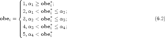
Table 11 shows the (Est.), standard deviation (Std), and 95% confidence interval (95% CI) of the regression coefficients and threshold estimates for the obesity risk data. As shown in the table, eight covariates of interest had different effects on BMI and obesity level. At three combinations of quantile levels, $τ_{1} = (0.5, 0.5)$ , $τ_{2} = (0.25, 0.75)$ , and $τ_{3} = (0.75, 0.25)$ , the effect of the covariates on these two responses was not identical. At three combinations of quantile levels, the variables of family history of obesity, frequency of vegetable consumption, and frequency of exercise had a significant effect on obesity level, and the variables of age, family history of obesity, frequency of vegetable consumption, and daily water consumption had a significant effect on BMI. Variables that also had a significant effect on BMI at the $τ_{1}$ and $τ_{2}$ levels include gender and frequency of consumption of high-calorie foods. Frequency of exercise had a significant effect on obesity and BMI at the $τ_{1}$ and $τ_{3}$ levels. The number of main meals consumed also had a significant effect on BMI at the $τ_{3}$ level. Positive and large regression coefficients of family history of obesity indicate that family members with a history of obesity may be at risk of obesity with higher obesity levels and BMI. Frequency of exercise had a significant effect on both obesity levels and BMI. Individuals with a higher frequency of exercise showed lower levels of obesity and BMI. For continuous response BMI, there was a significant difference in BMI between males and females. Within the age range of 14 to 55 of individuals in the dataset, there was a tendency toward increasing BMI with age. Frequency of consumption of high-calorie foods, frequency of vegetable consumption and daily water consumption had a positive effect on BMI, with individuals who consume a higher number of main meals showing lower levels of obesity and BMI. These results suggest that to decrease the risk of obesity, the consumption of high-calorie foods should be reduced, more main meals should be consumed, healthy diets should be accompanied by increased frequency of exercise, and obesity should be managed effectively, especially in individuals with a family history of obesity.

Table 11.

Parameter estimation results for the obesity risk dataset.

	$τ = (0.5, 0.5)$			$τ = (0.25, 0.75)$			$τ = (0.75, 0.25)$
Par.	Est.	Std	95%CI	Est.	Std	95%CI	Est.	Std	95%CI
Obesity level
$β_{11}$	−0.095	0.154	(−0.340,0.142)	0.016	0.163	(−0.303,0.323)	0.068	0.259	(−0.287,0.727)
$β_{12}$	0.027	0.018	(−0.001,0.058)	0.049	0.031	(0.004,0.112)	0.041	0.041	(−0.020,0.131)
$β_{13}$	1.850	0.301	(1.283,2.350)	1.197	0.593	(0.006,2.052)	2.330	0.423	(1.539,3.004)
$β_{14}$	0.732	0.487	(−0.087,1.664)	0.337	0.516	(−0.431,1.237)	0.324	0.492	(−0.153,1.571)
$β_{15}$	0.977	0.257	(0.437,1.474)	0.976	0.460	(−0.028,1.701)	1.137	0.413	(0.459,1.778)
$β_{16}$	0.085	0.137	(−0.071,0.387)	−0.006	0.175	(−0.220,0.181)	−0.064	0.187	(−0.505,0.231)
$β_{17}$	0.201	0.199	(−0.023,0.628)	0.438	0.280	(0.001,0.852)	0.265	0.332	(−0.155,0.887)
$β_{18}$	−0.075	0.116	(−0.318,−0.084)	−0.259	0.213	(−0.619,0.074)	−0.024	0.179	(−0.305,0.362)
$α_{1}$	0.047	0.035	(0.001,0.111)	0.101	0.081	(0.007,0.290)	0.047	0.043	(0.004,0.170)
$α_{2}$	1.996	0.097	(1.790,2.119)	2.060	0.137	(1.862,2.254)	1.956	0.033	(1.881,2.011)
$α_{3}$	3.738	0.200	(3.439,4.194)	4.008	0.193	(3.730,4.353)	3.956	0.280	(3.564,4.464)
$α_{4}$	5.417	0.142	(5.160,5.664)	5.363	0.231	(5.055,5.735)	5.407	0.155	(5.161,5.657)
Body mass index (BMI)
$β_{21}$	−0.677	0.395	(−1.480,−0.085)	−1.529	0.659	(−2.715,−0.459)	0.782	0.549	(−0.032,1.883)
$β_{22}$	0.228	0.049	(0.157,0.329)	0.143	0.061	(0.043,0.259)	0.430	0.048	(0.329,0.510)
$β_{23}$	13.075	0.669	(11.823,14.111)	14.504	1.100	(12.576,16.113)	7.202	1.085	(5.520,9.626)
$β_{24}$	4.767	0.815	(3.541,6.219)	3.921	0.888	(2.196,5.431)	0.209	0.421	(−0.432,1.339)
$β_{25}$	5.067	0.402	(4.384,5.651)	4.482	0.479	(3.717,5.301)	3.074	0.584	(2.145,4.391)
$β_{26}$	−0.031	0.142	(−0.393,0.222)	0.084	0.199	(−0.120,0.652)	−1.316	0.344	(−2.037,−0.699)
$β_{27}$	2.550	0.345	(1.874,3.101)	2.116	0.315	(1.637,2.809)	3.490	0.618	(2.380,4.831)
$β_{28}$	−0.481	0.531	(−1.291,0.751)	0.127	0.261	(−0.335,0.619)	−1.966	0.321	(−2.562,−1.360)

7. Conclusion

In this paper, we studied a joint QR model of mixed ordinal and continuous correlated responses based on the MAL distribution. In order to consider the correlation between mixed-type responses, we imposed a bivariate AL distribution for the error of ordinal response latent variable and continuous response in a linear regression framework. The model errors characterize the dependence between responses. Compared with the traditional univariate QR, the modeling approach in this paper allows for a more comprehensive study of different quantile levels combinations of mixed responses. In order to facilitate the implementation of Bayesian inference, we conducted Bayesian posterior inference via the MCMC algorithm using a hierarchical normal mixture representation of the MAL distribution and imposing $l_{1 / 2}$ penalty on the likelihood function of the joint distribution. In order to assess the effectiveness of the model proposed in this paper, Monte Carlo simulations were conducted, and the simulation results show that the model performs well. We also compared the joint QR model in this paper with a separate QR model, and the results confirm the validity of the joint model in analyzing mixed-type responses. Finally, we used the model to analyze real data on obesity risk.

Footnotes

Acknowledgments

Authors thank editors and two referees for their constructive comments and suggestions which have greatly improved the paper.

Declaration of conflicting interests

The authors declared no potential conflicts of interest with respect to the research, authorship, and/or publication of this article.

Funding

The authors received the following financial support for the research, authorship, and/or publication of this article: This research was joint supported by grants from National Natural Science Foundation of China (grant 12061065), National Foundation for Social Sciences of China (grant 22BTY037) and Funds for Innovative Fundamental Research Group Project of Gansu Province (grant 23JRRA684).

ORCID iDs

Yu-Zhu Tian

Mao-Zai Tian

Detailed derivation of the full conditional posterior distribution as follows

Derivation of the fully conditional posterior distribution of $β_{τ}$

\begin{aligned} π (β_{τ} | Ψ, λ, W_{i}) \\ \propto L_{C} (Z, Y_{1}, Y_{2}, W | β_{τ}, Ψ, α) \times π (β_{τ} | ω) \\ \propto \exp {- \frac{1}{2} \sum_{i = 1}^{N} {(Y_{i} - β_{τ} X_{i} - θ W_{i})}^{T} {(W_{i} Σ)}^{- 1} (Y_{i} - β_{τ} X_{i} - θ W_{i})} \times \prod_{j = 1}^{2} \prod_{k = 1}^{K} I (| β_{j, k} | < ω_{j, k}^{2}) \\ \propto \exp {- \frac{1}{2} t r \sum_{i = 1}^{N} {(β_{τ} X_{i} - C_{i})}^{T} {(W_{i} Σ)}^{- 1} (β_{τ} X_{i} - C_{i})} \times \prod_{j = 1}^{2} \prod_{k = 1}^{K} I (| β_{j, k} | < ω_{j, k}^{2}) \\ \propto \exp {- \frac{1}{2} [\sum_{i = 1}^{N} t r (W_{i}^{- 1} X_{i} X_{i}^{T} {β_{τ}}^{T} Σ^{- 1} β_{τ}) - 2 \sum_{i = 1}^{N} t r (W_{i}^{- 1} X_{i} C_{i}^{T} Σ^{- 1} β_{τ})]} \\ \times \prod_{j = 1}^{2} \prod_{k = 1}^{K} I (| β_{j, k} | < ω_{j, k}^{2}) \\ \propto \exp {- \frac{1}{2} t r [(\sum_{i = 1}^{N} W_{i}^{- 1} X_{i} X_{i}^{T}) \cdot {β_{τ}}^{T} Σ^{- 1} β_{τ} - 2 \sum_{i = 1}^{N} (W_{i}^{- 1} X_{i} C_{i}^{T} Σ^{- 1} β_{τ})]} \\ \times \prod_{j = 1}^{2} \prod_{k = 1}^{K} I (| β_{j, k} | < ω_{j, k}^{2}) \\ \propto \exp {- \frac{1}{2} t r [(\sum_{i = 1}^{N} W_{i}^{- 1} X_{i} X_{i}^{T}) \cdot {(β_{τ} - V)}^{T} Σ^{- 1} (β_{τ} - V)]} \times \prod_{j = 1}^{2} \prod_{k = 1}^{K} I (| β_{j, k} | < ω_{j, k}^{2}) \\ \propto \exp {- \frac{1}{2} t r (B^{- 1} \cdot {(β_{τ} - V)}^{T} Σ^{- 1} (β_{τ} - V))} \times \prod_{j = 1}^{2} \prod_{k = 1}^{K} I (| β_{j, k} | < ω_{j, k}^{2}) \\ \sim N_{2 \times k} (V, B \otimes Σ) . \end{aligned}

Derivation of the fully conditional posterior distribution of correlation matrix $Ψ$

\begin{aligned} π (Ψ | β_{τ}, W_{i}) \\ \propto L_{C} (Z, Y_{1}, Y_{2}, W | β_{τ}, Ψ, α) \times π (Ψ) \\ \propto \prod_{i = 1}^{N} \frac{1}{2 π {| W_{i} Δ Ψ Δ |}^{1 / 2}} \exp {- \frac{1}{2} \sum_{i = 1}^{N} η_{i}^{T} {(W_{i} Δ Ψ Δ)}^{- 1} η_{i}} \\ \times \frac{{| Ψ |}^{- (m_{0} + 3) / 2} \exp {- \frac{1}{2} t r (Ψ^{- 1} ψ_{0})}}{2^{m_{0}} {| ψ_{0} |}^{- m_{0} / 2} Γ_{2} (\frac{m_{0}}{2})} \\ \propto | Ψ |^{- (N + m_{0} + 3) / 2} \exp {- \frac{1}{2} [\sum_{i = 1}^{N} t r (η_{i}^{T} {(W_{i} Δ Ψ Δ)}^{- 1} η_{i}) + t r (Ψ^{- 1} ψ_{0})]} \\ \propto | Ψ |^{- (N + m_{0} + 3) / 2} \exp {- \frac{1}{2} t r [Ψ^{- 1} (Δ^{- 1} \sum_{i = 1}^{N} (W_{i}^{- 1} η_{i} η_{i}^{T}) Δ^{- 1} + ψ_{0})]} \\ \sim I W (N + m_{0}, Δ^{- 1} \sum_{i = 1}^{N} (W_{i}^{- 1} η_{i} η_{i}^{T}) Δ^{- 1} + ψ_{0}) . \end{aligned}

where

η_{i} = Y_{i} - β_{τ} X_{i} - θ W_{i} .

Derivation of fully conditional posterior distributions for latent variables $W_{i}$

\begin{aligned} π (W_{i} | β_{τ}, Ψ) \\ \propto L_{C} (Z, Y_{1}, Y_{2}, W | β_{τ}, Ψ, α) \times π (W_{i}) \\ \propto | W_{i} Σ |^{- 1 / 2} \exp {- \frac{1}{2} {(l_{i} - θ W_{i})}^{T} {(W_{i} Σ)}^{- 1} (l_{i} - θ W_{i})} \times \exp {- W_{i}} \\ \propto | W_{i} |^{- 1} \exp {- \frac{1}{2} [(l_{i}^{T} Σ^{- 1} l_{i}) W_{i}^{- 1} + (θ^{T} Σ^{- 1} θ + 2) W_{i}]} \\ \sim G I G (0, l_{i}^{T} Σ^{- 1} l_{i}, θ^{T} Σ^{- 1} θ + 2) . \end{aligned}

References

Sklar

. Random variables, distribution functions, and copulas: A personal look backward and forward. Lect Notes-Monogr Ser 1996; 28: 1–14.

Catalano

. Brivariate modelling of clustered continuous and ordered categorical outcomes. Stat Med 1997; 16: 883–900.

Gueorguieva

Sanacora

. Joint analysis of repeatedly observed continuous and ordinal measures of disease severity. Stat Med 2006; 25: 1307–1322.

Bahrami

Ganjali

Eftekhari

. A latent variable model for mixed continuous and ordinal responses with nonignorable missing responses: Assessing the local influence via covariance structure. Sankhya B 2010; 72: 38–57.

Teimourian

Baghfalaki

Ganjali

, et al. Joint modeling of mixed skewed continuous and ordinal longitudinal responses: A Bayesian approach. J Appl Stat 2015; 42: 2233–2256.

Buhule

Wahed

Youk

. Bayesian hierarchical joint modeling of repeatedly measured continuous and ordinal markers of disease severity: Application to Ugandan diabetes data. Stat Med 2017; 36: 4677–4691.

Ekvall

Molstad

. Mixed type multivariate response regression with covariance estimation. Stat Med 2022; 41: 2768–2785.

Baghfalaki

Ganjali

Kabir

, et al.A Bayesian shared parameter model for joint modeling of longitudinal continuous and binary outcomes. J Appl Stat 2022; 49: 638–655.

Ahmadi

Baghfalaki

Ganjali

, et al. A transition copula model for analyzing multivariate longitudinal data with missing responses. J Appl Stat 2022; 49: 3164–3177.

10.

Koenker

Bassett Jr

. Regression quantiles. Economet: J Economet Soc 1978; 46: 33–50.

11.

Moyeed

. Bayesian quantile regression. Stat Probab Lett 2001; 54: 437–447.

12.

Koenker

. Quantile regression for longitudinal data. J Multivar Anal 2004; 91: 74–89.

13.

Kozumi

Kobayashi

. Gibbs sampling methods for bayesian quantile regression. J Stat Comput Simul 2011; 81: 1565–1578.

14.

Tian

Zhu

. Linear quantile regression based on EM algorithm. Commun Stat-Theory Methods 2014; 43: 3464–3484.

15.

Waldmann

Kneib

. Bayesian bivariate quantile regression. Stat Modell 2015; 15: 326–344.

16.

Petrella

Raponi

. Joint estimation of conditional quantiles in multivariate linear regression models with an application to financial distress. J Multivar Anal 2019; 173: 70–84.

17.

Tian

Tang

Tian

. Bayesian joint inference for multivariate quantile regression model with

l_{1 / 2}

penalty. Comput Stat 2021; 36: 2967–2994.

18.

Merlo

Maruotti

Petrella

, et al. Quantile hidden semi-Markov models for multivariate time series. Stat Comput 2022; 32: 61.

19.

Ghasemzadeh

Ganjali

Baghfalaki

. Bayesian quantile regression for joint modeling of longitudinal mixed ordinal and continuous data. Commun Stat-Simul Comput 2020; 49: 375–395.

20.

Ghasemzadeh

Ganjali

Baghfalaki

. Quantile regression via the EM algorithm for joint modeling of mixed discrete and continuous data based on Gaussian copula. Stat Methods Appl 2022; 31: 1181–1202.

21.

Khazaei

Ganjali

Khazaei

. A Bayesian semi-parametric quantile regression approach for joint modeling of longitudinal ordinal and continuous responses. Stat Optimiz Inf Comput 2023; 11: 445–464.

22.

Tibshirani

. Regression shrinkage and selection via the lasso. J R Stat Soc Ser B: Stat Methodol 1996; 58: 267–288.

23.

Fan

. Variable selection via nonconcave penalized likelihood and its oracle properties. J Am Stat Assoc 2001; 96: 1348–1360.

24.

Zou

Hastie

. Regularization and variable selection via the elastic net. J R Stat Soc Ser B: Stat Methodol 2005; 67: 301–320.

25.

Zou

. The adaptive lasso and its oracle properties. J Am Stat Assoc 2006; 101: 1418–1429.

26.

Huang

Horowitz

. Asymptotic properties of bridge estimators in sparse high-dimensional regression models. Ann Stat Ann Statist 2008; 36: 587–613.

27.

Zhang

. Nearly unbiased variable selection under minimax concave penalty. Ann Stat 2010; 38: 894–942.

28.

Chang

l_{1 / 2}

regularization: A thresholding representation theory and a fast solver. IEEE Trans Neural Netw Learn Syst 2012; 23: 1013–1027.

29.

Rothman

Levina

Zhu

. Sparse multivariate regression with covariance estimation. J Comput Graph Stat 2010; 19: 947–962.

30.

Chen

Kang

Jin

, et al.Bayesian sparse regression for mixed multi-responses with application to runtime metrics prediction in fog manufacturing. Technometrics 2023; 65: 206–219.

31.

Wang

Bai

Huang

. Mixed-type multivariate bayesian sparse variable selection with shrinkage priors.arxiv preprint arxiv:2201. 12839, 2023.