Quantile regressions offer several attractive features, including the ability to allow covariate effects to vary at different quantile levels and to effectively handle heteroscedasticity in data, which makes it a viable alternative for analyzing data with continuous outcomes in recent years. It has been used in modeling survival data with and without a cured fraction. In this work, we propose novel estimating equation approaches to estimate a mixture cure model where the latency survival time is modeled using a quantile regression. Our proposed estimation methods provide double robustness, meaning that a misspecification in one part of the mixture cure model will not affect the estimation in the other part. The methods relax the restrictive global log-linear assumption that is typically found in existing quantile regressions, and they allow for both quantile-varying and quantile-invariant effects in the regression when the log-linear assumption holds within a certain range of quantile levels. We established the asymptotic properties of the proposed estimators, and our simulation studies demonstrated their double robustness and efficiency gains. An application of the proposed model and methods to data from a lung cancer study revealed that uncured patients with adenocarcinoma have significantly longer quantiles in the survival time than uncured patients with squamous cell carcinoma, which had not been reported in previous analyses of the data due to the limitations of the existing methods.
Analyzing survival data to assess the effects of covariates on the quantiles, rather than on the mean or the hazard rate of the time until an event occurs, has gained popularity in recent years. This approach provides a more intuitive interpretation of effects compared to traditional survival models, such as Cox’s proportional hazards (PH) model.1 Additionally, it allows for variation in effects at different quantiles, making it more flexible than models like an accelerated failure time (AFT) model,2 which assumes constant effects of covariates across quantiles. When estimating the effects on quantiles for survival data, it is crucial to consider potential cured subjects who may never experience the event of interest, as these subjects should not contribute to the estimation of the effects.
Consider a lung cancer study3 where the event of interest is death due to lung cancer, and one is interested in the effects of tumor histology, sex, and age on the quantiles of the time to death due to lung cancer. Figure A.1 in the Supplementary materials of Wu and Yin3 shows the estimated Kaplan–Meier survival curves stratified by tumor histology. These curves display a distinct plateau at the right tail, suggesting the presence of cured patients who may never die due to lung cancer in this study. It is essential to separate the impact of the cured patients from estimating the effects of the covariates on the time to death due to lung cancer. Wu and Yin3 analyzed the data using a quantile mixture cure model. Although they found an age effect on the probability of being cured, they did not find any significant effects among tumor histology, sex, and age on the time to death due to lung cancer, which is likely due to the issues in the existing methods that are discussed below.
Recent developments in quantile regressions for censored survival data with a cured fraction present an opportunity to model covariate effects on the quantile of an uncured subject’s survival time. Based on the work of Peng and Huang,4 Wu and Yin5 introduced a cure rate quantile regression and proposed a two-stage estimation method, where Stage 1 estimates the probability of being cured and Stage 2 estimates the covariate effects on the quantile of the time to the event of interest among uncured subjects using the results from Stage 1. However, similar to the method in Peng and Huang,4 the two-stage method relies on a global linearity assumption across all quantile levels. To relax the assumption, Wu and Yin3 developed a multiple imputation method that utilizes the locally weighted quantile regression approach of Wang and Wang6 in Stage 2. Despite this advancement, the nonparametric kernel smoothing technique used in both stages, alongside the multiple imputation method, makes the method computationally demanding. The estimation in Stage 2 requires consistent estimation results in Stage 1. Thus, a misspecification in Stage 1 can have a nonignorable impact on the quantile regression estimation in Stage 2. Furthermore, the kernel smoothing technique can struggle with the curse of dimensionality in practical applications. Recently, Narisetty and Koenker7 developed a new data augmentation method that generalizes the approach of Yang et al.8 for survival data with a cure fraction. Nevertheless, this method still requires the global linearity assumption.
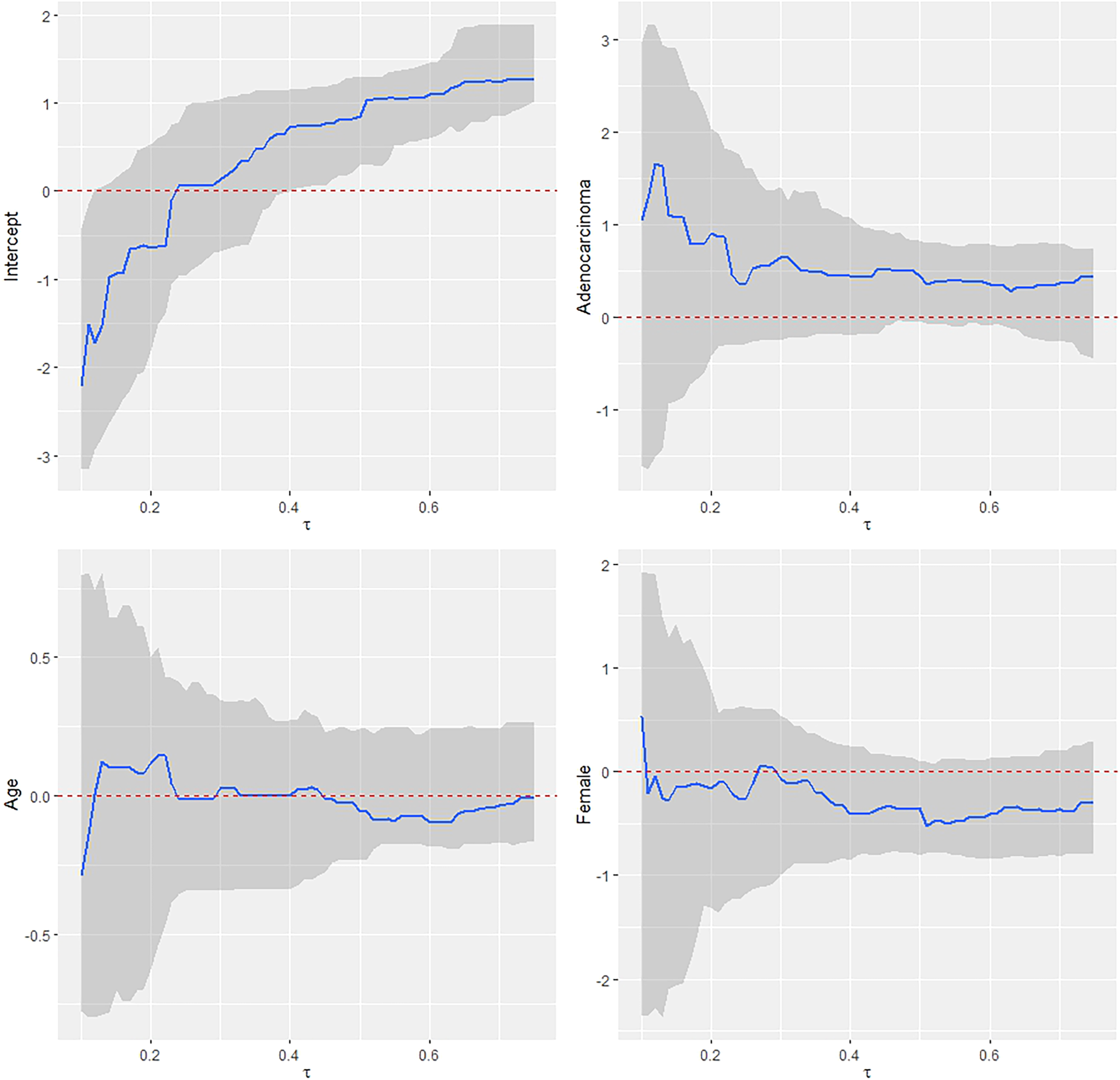
Another significant issue with current methods for quantile cure models is that they assume all covariate effects on the quantiles of the time to the event of interest are quantile-varying (or functional) covariate effects. However, some covariates may actually have quantile-invariant (or homogeneous) effects, leading to a loss of estimation efficiency. This is evident in the lung cancer study mentioned earlier. The estimated effects of histology, sex, and age on the quantiles of the time to death due to lung cancer do not vary substantially across a wide range of quantiles (see Figure 1), suggesting that a model allowing for partially functional covariate effects on the quantiles would be beneficial. If the quantile effects of some covariates do not vary in an interval of quantiles, limiting the quantile-varying effects to those covariates that actually exhibit such variability could improve estimation efficiency.
Estimated fully functional covariate effects for uncured patients using the quantile cure model for the lung cancer data.
Without a cured fraction, Qian and Peng9 allowed for constant effects for some covariates but imposed a strong assumption of global linearity. Chu and Sit10 recently developed a new quantile model for survival data that permits local homogeneity across a specified range of quantiles for all covariates. However, the homogeneity assumption applied to all covariates may be too restrictive in practical situations. Furthermore, it remains unclear how to extend their method to data with a cured fraction.
The issues mentioned above motivate us to propose a new quantile cure model that incorporates partially functional covariate effects. This model combines quantile-varying effects and quantile-invariant effects on the quantiles of the time to event of interest among uncured subjects. It allows for a linear assumption within a subinterval of quantile values, rather than across all quantile values, and quantile-invariant effects for some covariates. The partially functional covariate effects we suggest are more flexible than the fully functional covariate effects described in previous works. We develop a new estimation method based on estimating equations and the inverse probability of censoring weighting (IPCW). This method separately estimates the effects of covariates on the probability of being cured and on the time to the event of interest among uncured subjects. The separate estimation in the two parts ensures that the estimation in one part is robust to the misspecification in the other part. Our method relies on neither the kernel-smoothed estimation nor the multiple imputation and therefore is easy to implement. We also explore the asymptotic properties of the estimates. Additionally, we propose a test procedure to determine whether a covariate has a homogeneous effect within that interval. The merit of the proposed method is demonstrated in the lung cancer study, where the method finds a significant effect of histology on the time to death due to lung cancer among uncured patients.
The paper is organized as follows. Section 2 presents the data structure and the local quantile effect cure model, in which a quantile regression at a specific quantile level is specified for an uncured subject. Two estimating equations for the two parts of the cure model are developed, and the asymptotic properties of the proposed estimators are derived. When the linearity assumption holds for all covariates on a quantile range of interest, an inference method is presented in Section 3, and the large sample properties of the estimates are established. This method is further extended to the partially functional covariate effects when some covariates have constant quantile effects. Extensive simulation studies are carried out in Section 4 to evaluate the performance of the proposed methods. In Section 5, the data from the motivating lung cancer study are analyzed using the proposed model and estimation method as an illustration. Section 6 concludes this article with some remarks.
Local quantile effect cure model
Model assumptions
Let denote the cure status of an individual. An individual with will eventually experience the event of interest with event time if there is no censoring, while an individual with is cured with survival time equal to , indicating that the individual will never experience the event of interest. Hence, the failure time of an individual can be written as . In practice, there may exist a censoring time and a finite administrative censoring time such that can be righted censored by . Let and . An individual with is known to be uncured and . However, the cure status of an individual with is unknown. Let be a set of covariates that may have effects on , , and , and assume that is independent of and given . Let observed data be independent and identically distributed () copies of .
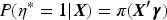
Assume that the uncured probability is associated with a -vector of covariates
where the first component of is 1 corresponding to the intercept, is the effect of , and : is a known function of . This is often referred to as the incidence part of the cure model. There are many choices for the function . If , the incidence part assumes the logistic regression. If or , the incidence part specifies the probit regression or the complementary log–log model, respectively, where is the cumulative distribution function of a standard normal random variable.
For the distribution of , let be a quantile level of interest and denote the th quantile of given . Assume that at the specific , is modeled by
where is the effect of and contains an intercept. This is often referred to as the latency part of the cure model. Model (2) only requires the linearity between and at a specific quantile level , and it does not require the global linearity assumption on (0, 1). We consider the exponential function to link between and in (2). However, other increasing functions can be considered here, such as the inverse of the Box–Cox transformation,11 which contains an unknown parameter to be estimated. Further research is warranted for a more flexible transformation function in (2).
Estimation for the incidence part
Let be the true value of . Since implies and , using the conditional independence between and given and following Chen et al.,12 we have the following equation where is the survival function of censoring time that may depend on . If is a consistent estimator of , we have the following estimating equation for
Let be the root of (3) and be the estimated uncured probability of subject .
Estimation for the latency part
To estimate , consider . Hence, implies that
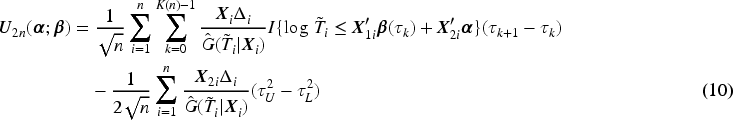
can be an estimating equation for . In view of (3), we have and plug this in (4), which motivates us to construct the following estimating equation for at a given
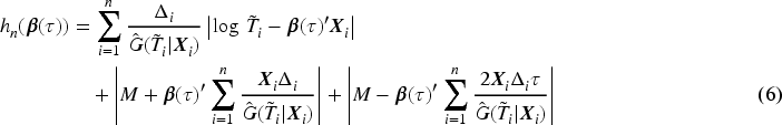
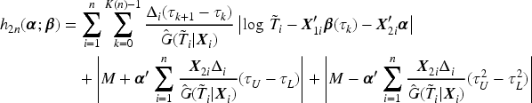
Let , the root of (5), denote the proposed estimator of . Since there may exist multiple roots or no root for (5), we treat as a generalized solution of (5), which is equivalent to finding the minimizer of the following -type convex function
We suggest estimating using the Kaplan–Meier estimator if it does not depend on . If depends on , we may model with some survival models, for example, Cox’s PH model, the AFT model, or a nonparametric estimation method14 to take the effect of into account in the estimate . When modeling survival data with a cure model, the support of is required to cover the support of to meet the sufficient follow-up requirement so that the cure probability can be properly estimated from the data.15,16 Hence, consistency and the weak convergence property of hold on the support of 17 because the estimate of will be a proper survival function, and it is well defined for a time within the support of .
The asymptotic properties of have been investigated in Chen et al.12 and its asymptotic variance can be estimated by applying the plug-in method. We established the consistency and the asymptotic normality of . The details of the asymptotic properties and their proof are relegated to Section A in the Supplemental materials. Following Peng and Fine,13 the plug-in estimator for the asymptotic variances can be derived. However, according to our simulation experience, the variance estimate for using the plug-in method is not reliable and can sometimes cause a smaller empirical coverage rate than 95% for the Wald-type 95% confidence interval based on the variance estimate. This is also reported and discussed by Choi et al.18 Consequently, we suggest applying the weighted bootstrap approach19 for the variance estimation. The details of this approach are provided in Section B in the Supplemental materials.
It is noteworthy that our approach is fundamentally different from that of Wu and Yin.3 Wu and Yin3 developed a two-stage estimation method, where is estimated in Stage 1 and then is estimated in Stage 2 using the multiple imputation and the results from Stage 1. The local Kaplan–Meier estimators for the latency survival function are repeatedly used in both stages. However, the locally nonparametric estimator suffers from the curse of dimensionality. Moreover, the estimation in the latency part of their method requires consistent estimation results in Stage 1. Thus, a misspecification in the incidence part can have a nonignorable impact on the quantile regression estimation in Stage 2. In contrast, in our proposed approach, the estimation in one part does not depend on the other part. This can be seen from the fact that the estimating equation (3) does not depend on the latency part and the estimating equation (5) does not depend on the incidence part, which makes the estimation doubly robust to the misspecification of either part of the model. This advantage holds for the quantile cure model only because is equal to the common for all . A disadvantage of the proposed method is that we need to estimate the censoring distribution. If the censoring mechanism depends on a high-dimensional set of covariates in a way that cannot be sufficiently modeled by the Cox PH or the AFT models, and a nonparametric estimation has to be considered, then the proposed method may also suffer from the curse of dimensionality. However, this concern is at a much lesser degree than that in the method of Wu and Yin3 because the censoring time is usually considered separately from the event time of interest, and it is not uncommon to assume a simpler model for the association between and a limited number of covariates. On the other hand, Wu and Yin3 suggested modeling nonparametrically. The function is for the event of interest, and if is high-dimensional, the concern of the curse of dimensionality will inevitably arise. Moreover, this approach basically considered two models for , one is the conditional quantile model and the other is the nonparametric estimation method. There is no guarantee that the two models produce coherent estimates, which can in turn affect the final estimates adversely.
Functional covariate effects
Fully functional covariate effects
If the linearity assumption (2) holds for all covariates over a range of quantiles in , where , can be estimated from (5). We consider as a right-continuous step function of at artificially selected jump points and estimate , in a pointwise manner using the estimating equation (5) and computation algorithm (6). One advantage of our approach is that the estimation of at does not require to be carried out sequentially from lower quantiles. We set the mesh size as order of . Under regularity conditions, we can prove that the estimator on is uniformly consistent on and converges to a Gaussian process at a root- rate. The details of the asymptotic properties and their proof are provided in Section C in the Supplemental materials.
Partially functional covariate effects
The fully functional covariate effects in Section 3.1 assume that the effect in (2) holds for all covariates in on . However, in practice, the quantile effects of some covariates may be invariant over the range . To make the estimation more efficient, it is important to take this information into account in the estimation procedure. Let , where is a -dimensional covariate vector with quantile-varying effect and is a -dimensional covariate vector with quantile-invariant effects , where . The quantile regression model in the latency part assumes the partially functional covariate effects
for all . For the sake of simplicity, the intercept of the model is included in , and thus the first component of is 1.
Similar to Section 2, we assume that the observed data are copies of . The estimating equation of in the incidence part is still (3). The estimating equation for for any can be obtained from (5) as
Similar to the fully functional covariate effects, we consider the estimator of as a right-continuous step function of with jumps in . To estimate , we take the quantile-invariant information into account and derive the following estimating equation
Similar to the method proposed for (5), we obtain an estimate of as a generalized solution of (8), which is equivalent to searching for the minimizer of the following function
where is a very large number. Given the fact that the estimator of is a right-continuous step function of , the terms in can be rearranged as
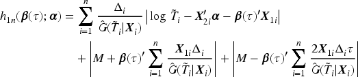
Then, an estimator of as the root of (10) can be obtained by finding the minimizer of the following function
The algorithm iterates between minimizing to update and minimizing to update until a predetermined convergence criterion is met. We denote the final estimators by . Under regularity conditions, we can prove the consistency of and the uniform consistency of . Both have a weak convergence. The details of the asymptotic properties and their proof are provided in Section D in the Supplemental materials. The variance estimation of follows the same resampling approach described in Section 2.3. When using , the initial value of may be obtained as the average of the functional effects of across all possible ’s. Then, the estimate of can be used in to update . To start the iterative estimation procedure, one can set and (except for the intercept ) as the initial values. An initial value of can be set to , where is an estimate of the survival function of , which can be estimated by , is the Kaplan–Meier survival estimate based on the observed data , and .
The choice of in the interval is very crucial, since it may cause the nonidentifiability issue and affect the estimation of and if it is too wide. Wu and Yin5 proposed an adaptive approach to select the largest such that and the identifiability of the parameters for are ensured, and this approach can be employed here.
We considered methods to check the fits of the proposed models for all . There are a few methods proposed in the literature to check the fit of a cure model. We adapted the Cox–Snell residuals proposed for the mixture cure model by Peng and Taylor.20 Let . The residual for subject based on an estimated cure model is defined as . It is proved that if the estimated cure model fits the data well for all , the residual can be viewed as a random number from a mixed-type distribution with a unit exponential distribution as the continuous component on and a probability mass at . The distribution of the censored residuals , , can be compared with the unit exponential distribution to determine the fit of the estimated cure model and this is usually done by plotting the estimated cumulative hazard function of the censored residuals and comparing it with a line. This approach, however, cannot be applied directly to the proposed model as the proposed method does not estimate . We proposed the following approach to approximate the residuals: Consider grid points , between . We use the proposed method to estimate and all , , and then estimate by if . The corresponding Cox–Snell residual for the subject is obtained as . If the model contains an estimated quantile-invariant effect , then is determined by . We suggest that .
Selecting covariates with partially or fully functional effects
An interesting question in practice is how to choose between and for a set of covariates. We suggest that a model with all covariates in should be fit first, and then the plot of each estimate in against is visually examined and followed by a hypothesis test to examine the significance of the quantile-varying effect in an interval identified in the visual inspection. If the plot of an estimate does not show a substantial change in the interval and the test shows no significant quantile-varying effect, the corresponding covariate is moved from to . This approach provides investigators with a method to select a parsimonious quantile model in the latency part and efficiently summarizes the effect of a covariate via one parameter instead of a quantile-varying effect when it is unnecessary.
To test whether or not a covariate has a quantile-varying effect in a prespecified interval, we follow the approach proposed by Peng and Huang4 to conduct hypothesis testing. Suppose that we are interested in testing the significance of the quantile-varying effect in for the th covariate in over the interval . The hypotheses are
where is an unspecified constant. Let be a weight function. We propose the following test statistic
where . If this test statistic is further away from zero, it tends to reject the null hypothesis. Under , the distribution of can be approximated by the weighted bootstrap approach. After obtaining from the th bootstrap sample, , calculate , where . Then, the hypothesis is rejected if is smaller than 2.5th quantile or larger than 97.5th quantile of , under the 0.05 significance level. An example of the weight function is . Other types of the weight function, such as , can be considered too. If the null hypothesis cannot be rejected, it implies that the quantile-varying effect of is not significant, and the corresponding covariate should be considered in with a quantile-invariant or homogeneous effect.
Simulation studies
Covariate effects on quantiles
We consider , where and are respectively generated independently of the Bernoulli distribution with success probability 0.5 and uniform distribution on . Three link functions for in (1) are considered in data generation:
the logit link ,
the probit link ,
the complementary log–log link ,
with . These three link functions respectively produce 72%, 80%, and 88% as the average of uncure rates. For the latency part, assume with . It implies . Two types of distributions for are considered: the standard normal distribution with and the extreme value distribution with . When follows the standard normal distribution, , . When follows the extreme value distribution, , . The censoring time follows a mixture distribution with 80% from the exponential distribution with a rate of 0.025 and right-truncated at time 80 and 20% from a degenerated distribution at 80 if follows the standard normal distribution or a mixture distribution with 80% from the exponential distribution with a rate of 0.025 and right-truncated at time 60 and 20% from a degenerated distribution at 60 if follows the extreme value distribution. The resulting censoring rate among the uncured subjects is about 12% if follows the standard normal distribution and 8% if follows the extreme value distribution. The overall average censoring rates are respectively 36%, 29%, and 21% for the logit, probit, and complementary log–log links in the incidence parts if follows the standard normal distribution, and 34%, 25%, and 18% if follows the extreme value distribution. Additional simulation studies with higher censoring rates are provided in Section E in the Supplemental materials.
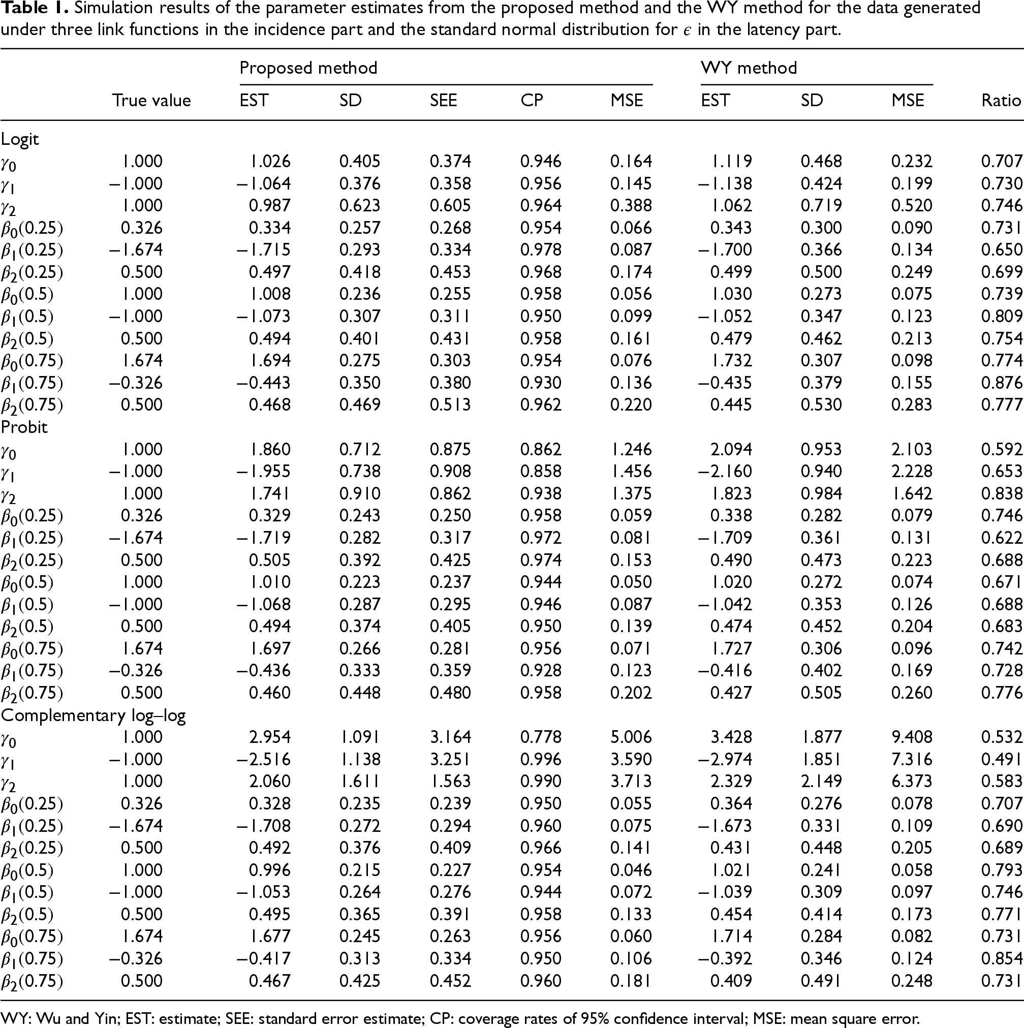
We generate 500 Monte Carlo datasets with a sample size of for each data configuration. For each dataset, the estimation method in Section 2 is used to estimate and with the logit link used in the incidence part (an R program was developed for the proposed estimation methods and tests, and it is available in the Supplemental materials). Consequently, our approach correctly specifies the incidence part in case (i), but misspecifies it in cases (ii) and (iii). The standard error estimates SEEs for are based on the weighted bootstrap method with , while those for are based on the plug-in type standard error estimator of Chen et al.12 The 95% confidence intervals for are based on the 2.5th and 97.5th percentiles from the weighted bootstrap estimates. The simulation results for following the standard normal distribution and extreme value distribution are respectively summarized in Tables 1 and 2. Both tables include the average estimates (EST), the sample standard deviations (SD), the averages of the SEEs, and the coverage rates of 95% confidence intervals (CP), and the mean square errors (MSEs) from the proposed method. We also fit the data using the method proposed by Wu and Yin3 (referred to as the WY method) for comparison, but only report ESTs, SDs, and MSEs to save time. The biquadratic kernel function with 10 imputation times is used in the WY method. The relative efficiency is measured by the ratios of MSEs of the proposed method to those of the WY method.
Simulation results of the parameter estimates from the proposed method and the WY method for the data generated under three link functions in the incidence part and the standard normal distribution for in the latency part.
Proposed method
WY method
True value
EST
SD
SEE
CP
MSE
EST
SD
MSE
Ratio
Logit
1.000
1.026
0.405
0.374
0.946
0.164
1.119
0.468
0.232
0.707
−1.000
−1.064
0.376
0.358
0.956
0.145
−1.138
0.424
0.199
0.730
1.000
0.987
0.623
0.605
0.964
0.388
1.062
0.719
0.520
0.746
0.326
0.334
0.257
0.268
0.954
0.066
0.343
0.300
0.090
0.731
−1.674
−1.715
0.293
0.334
0.978
0.087
−1.700
0.366
0.134
0.650
0.500
0.497
0.418
0.453
0.968
0.174
0.499
0.500
0.249
0.699
1.000
1.008
0.236
0.255
0.958
0.056
1.030
0.273
0.075
0.739
−1.000
−1.073
0.307
0.311
0.950
0.099
−1.052
0.347
0.123
0.809
0.500
0.494
0.401
0.431
0.958
0.161
0.479
0.462
0.213
0.754
1.674
1.694
0.275
0.303
0.954
0.076
1.732
0.307
0.098
0.774
−0.326
−0.443
0.350
0.380
0.930
0.136
−0.435
0.379
0.155
0.876
0.500
0.468
0.469
0.513
0.962
0.220
0.445
0.530
0.283
0.777
Probit
1.000
1.860
0.712
0.875
0.862
1.246
2.094
0.953
2.103
0.592
−1.000
−1.955
0.738
0.908
0.858
1.456
−2.160
0.940
2.228
0.653
1.000
1.741
0.910
0.862
0.938
1.375
1.823
0.984
1.642
0.838
0.326
0.329
0.243
0.250
0.958
0.059
0.338
0.282
0.079
0.746
−1.674
−1.719
0.282
0.317
0.972
0.081
−1.709
0.361
0.131
0.622
0.500
0.505
0.392
0.425
0.974
0.153
0.490
0.473
0.223
0.688
1.000
1.010
0.223
0.237
0.944
0.050
1.020
0.272
0.074
0.671
−1.000
−1.068
0.287
0.295
0.946
0.087
−1.042
0.353
0.126
0.688
0.500
0.494
0.374
0.405
0.950
0.139
0.474
0.452
0.204
0.683
1.674
1.697
0.266
0.281
0.956
0.071
1.727
0.306
0.096
0.742
−0.326
−0.436
0.333
0.359
0.928
0.123
−0.416
0.402
0.169
0.728
0.500
0.460
0.448
0.480
0.958
0.202
0.427
0.505
0.260
0.776
Complementary log–log
1.000
2.954
1.091
3.164
0.778
5.006
3.428
1.877
9.408
0.532
−1.000
−2.516
1.138
3.251
0.996
3.590
−2.974
1.851
7.316
0.491
1.000
2.060
1.611
1.563
0.990
3.713
2.329
2.149
6.373
0.583
0.326
0.328
0.235
0.239
0.950
0.055
0.364
0.276
0.078
0.707
−1.674
−1.708
0.272
0.294
0.960
0.075
−1.673
0.331
0.109
0.690
0.500
0.492
0.376
0.409
0.966
0.141
0.431
0.448
0.205
0.689
1.000
0.996
0.215
0.227
0.954
0.046
1.021
0.241
0.058
0.793
−1.000
−1.053
0.264
0.276
0.944
0.072
−1.039
0.309
0.097
0.746
0.500
0.495
0.365
0.391
0.958
0.133
0.454
0.414
0.173
0.771
1.674
1.677
0.245
0.263
0.956
0.060
1.714
0.284
0.082
0.731
−0.326
−0.417
0.313
0.334
0.950
0.106
−0.392
0.346
0.124
0.854
0.500
0.467
0.425
0.452
0.960
0.181
0.409
0.491
0.248
0.731
WY: Wu and Yin; EST: estimate; SEE: standard error estimate; CP: coverage rates of 95% confidence interval; MSE: mean square error.
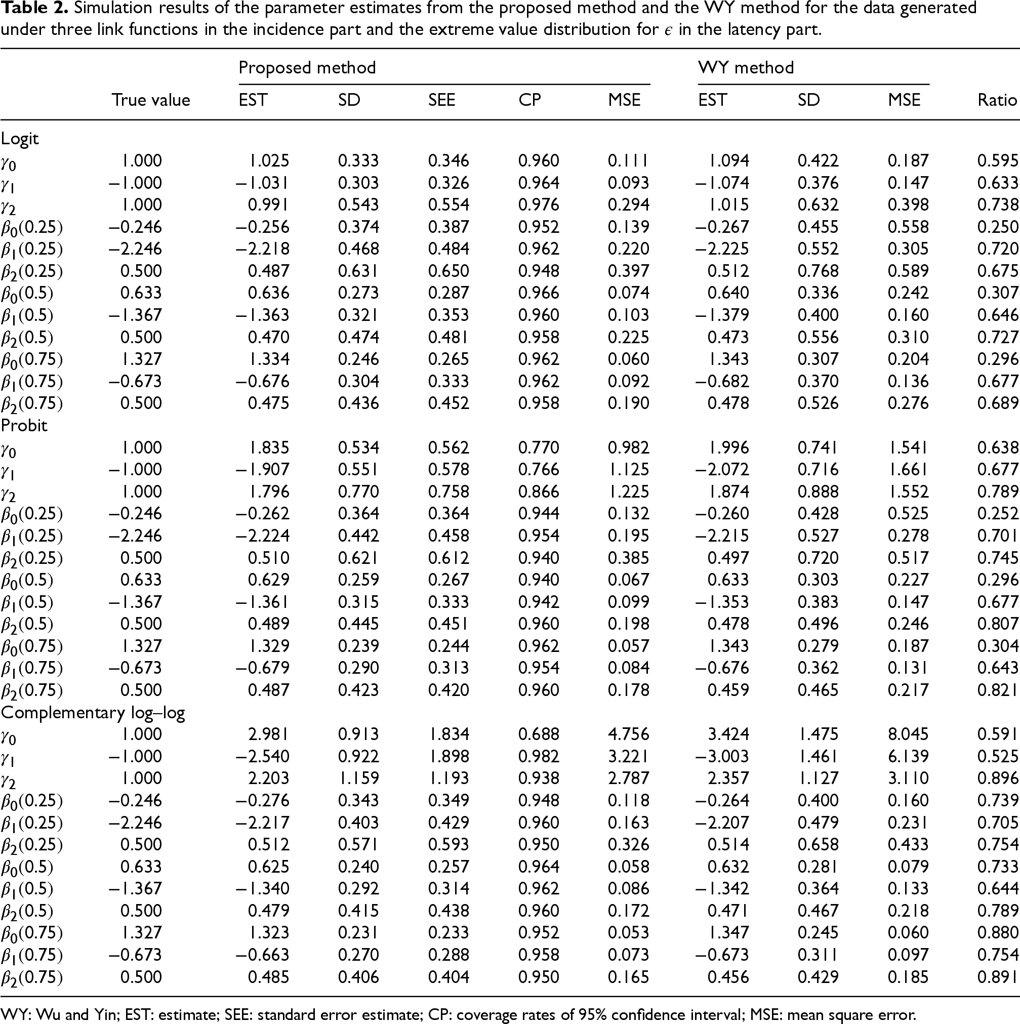
Simulation results of the parameter estimates from the proposed method and the WY method for the data generated under three link functions in the incidence part and the extreme value distribution for in the latency part.
Proposed method
WY method
True value
EST
SD
SEE
CP
MSE
EST
SD
MSE
Ratio
Logit
1.000
1.025
0.333
0.346
0.960
0.111
1.094
0.422
0.187
0.595
−1.000
−1.031
0.303
0.326
0.964
0.093
−1.074
0.376
0.147
0.633
1.000
0.991
0.543
0.554
0.976
0.294
1.015
0.632
0.398
0.738
−0.246
−0.256
0.374
0.387
0.952
0.139
−0.267
0.455
0.558
0.250
−2.246
−2.218
0.468
0.484
0.962
0.220
−2.225
0.552
0.305
0.720
0.500
0.487
0.631
0.650
0.948
0.397
0.512
0.768
0.589
0.675
0.633
0.636
0.273
0.287
0.966
0.074
0.640
0.336
0.242
0.307
−1.367
−1.363
0.321
0.353
0.960
0.103
−1.379
0.400
0.160
0.646
0.500
0.470
0.474
0.481
0.958
0.225
0.473
0.556
0.310
0.727
1.327
1.334
0.246
0.265
0.962
0.060
1.343
0.307
0.204
0.296
−0.673
−0.676
0.304
0.333
0.962
0.092
−0.682
0.370
0.136
0.677
0.500
0.475
0.436
0.452
0.958
0.190
0.478
0.526
0.276
0.689
Probit
1.000
1.835
0.534
0.562
0.770
0.982
1.996
0.741
1.541
0.638
−1.000
−1.907
0.551
0.578
0.766
1.125
−2.072
0.716
1.661
0.677
1.000
1.796
0.770
0.758
0.866
1.225
1.874
0.888
1.552
0.789
−0.246
−0.262
0.364
0.364
0.944
0.132
−0.260
0.428
0.525
0.252
−2.246
−2.224
0.442
0.458
0.954
0.195
−2.215
0.527
0.278
0.701
0.500
0.510
0.621
0.612
0.940
0.385
0.497
0.720
0.517
0.745
0.633
0.629
0.259
0.267
0.940
0.067
0.633
0.303
0.227
0.296
−1.367
−1.361
0.315
0.333
0.942
0.099
−1.353
0.383
0.147
0.677
0.500
0.489
0.445
0.451
0.960
0.198
0.478
0.496
0.246
0.807
1.327
1.329
0.239
0.244
0.962
0.057
1.343
0.279
0.187
0.304
−0.673
−0.679
0.290
0.313
0.954
0.084
−0.676
0.362
0.131
0.643
0.500
0.487
0.423
0.420
0.960
0.178
0.459
0.465
0.217
0.821
Complementary log–log
1.000
2.981
0.913
1.834
0.688
4.756
3.424
1.475
8.045
0.591
−1.000
−2.540
0.922
1.898
0.982
3.221
−3.003
1.461
6.139
0.525
1.000
2.203
1.159
1.193
0.938
2.787
2.357
1.127
3.110
0.896
−0.246
−0.276
0.343
0.349
0.948
0.118
−0.264
0.400
0.160
0.739
−2.246
−2.217
0.403
0.429
0.960
0.163
−2.207
0.479
0.231
0.705
0.500
0.512
0.571
0.593
0.950
0.326
0.514
0.658
0.433
0.754
0.633
0.625
0.240
0.257
0.964
0.058
0.632
0.281
0.079
0.733
−1.367
−1.340
0.292
0.314
0.962
0.086
−1.342
0.364
0.133
0.644
0.500
0.479
0.415
0.438
0.960
0.172
0.471
0.467
0.218
0.789
1.327
1.323
0.231
0.233
0.952
0.053
1.347
0.245
0.060
0.880
−0.673
−0.663
0.270
0.288
0.958
0.073
−0.673
0.311
0.097
0.754
0.500
0.485
0.406
0.404
0.950
0.165
0.456
0.429
0.185
0.891
WY: Wu and Yin; EST: estimate; SEE: standard error estimate; CP: coverage rates of 95% confidence interval; MSE: mean square error.
The results in both tables show that when the link function in the incidence part is correctly specified, that is, in the logit link case, the estimates of the proposed method are approximately unbiased, SEE is close to SD, and the coverage probabilities are close to the nominal level. The estimates from the proposed method have smaller SD and MSE than those from the WY method, and the MSE ratios are about 70% to 88%, indicating that the proposed method gains substantial efficiency over the WY method in this case. When the link function in the incidence part is misspecified by both methods, that is, in the probit and complementary log–log link function cases, the estimates of from the proposed method are still robust and have smaller MSEs than those from the WY method. It is noteworthy that the biases in and tend to be larger in both methods for the cases of standard normally distributed than those of extreme value distributed . It may be related to a higher censoring rate in the former than that in the latter such that the former provides less information for estimating when is large. In both tables, most of the estimates of from the proposed method have smaller biases than those from the WY method, indicating that the proposed method tends to be more robust to the misspecification of the incidence part.
It is not unexpected that the estimates of do not perform well under the probit and the complementary log–log links because of the misspecified model for the incidence part.
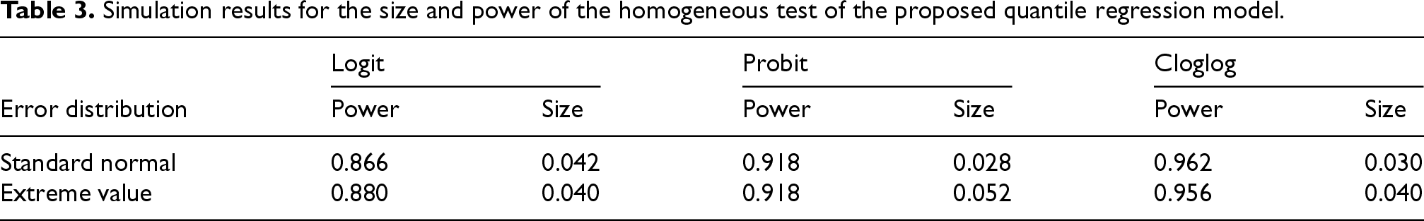
We further investigated the performance of the test (12) proposed in Section 3.3 to test the significance of quantile-varying effects. In the settings considered above, is a quantile-varying effect while is quantile-invariant. Thus, we can see the power and the size of the test when applying the test to the simulated data to test and respectively. When using the test, we set , where . The results are presented in Table 3. They show that the power of the test is good and the size of the test is slightly conservative. The results are insensitive to the error distribution choices and the specification of the link function in the incidence part.
Simulation results for the size and power of the homogeneous test of the proposed quantile regression model.
Logit
Probit
Cloglog
Error distribution
Power
Size
Power
Size
Power
Size
Standard normal
0.866
0.042
0.918
0.028
0.962
0.030
Extreme value
0.880
0.040
0.918
0.052
0.956
0.040
Partially functional covariate effects
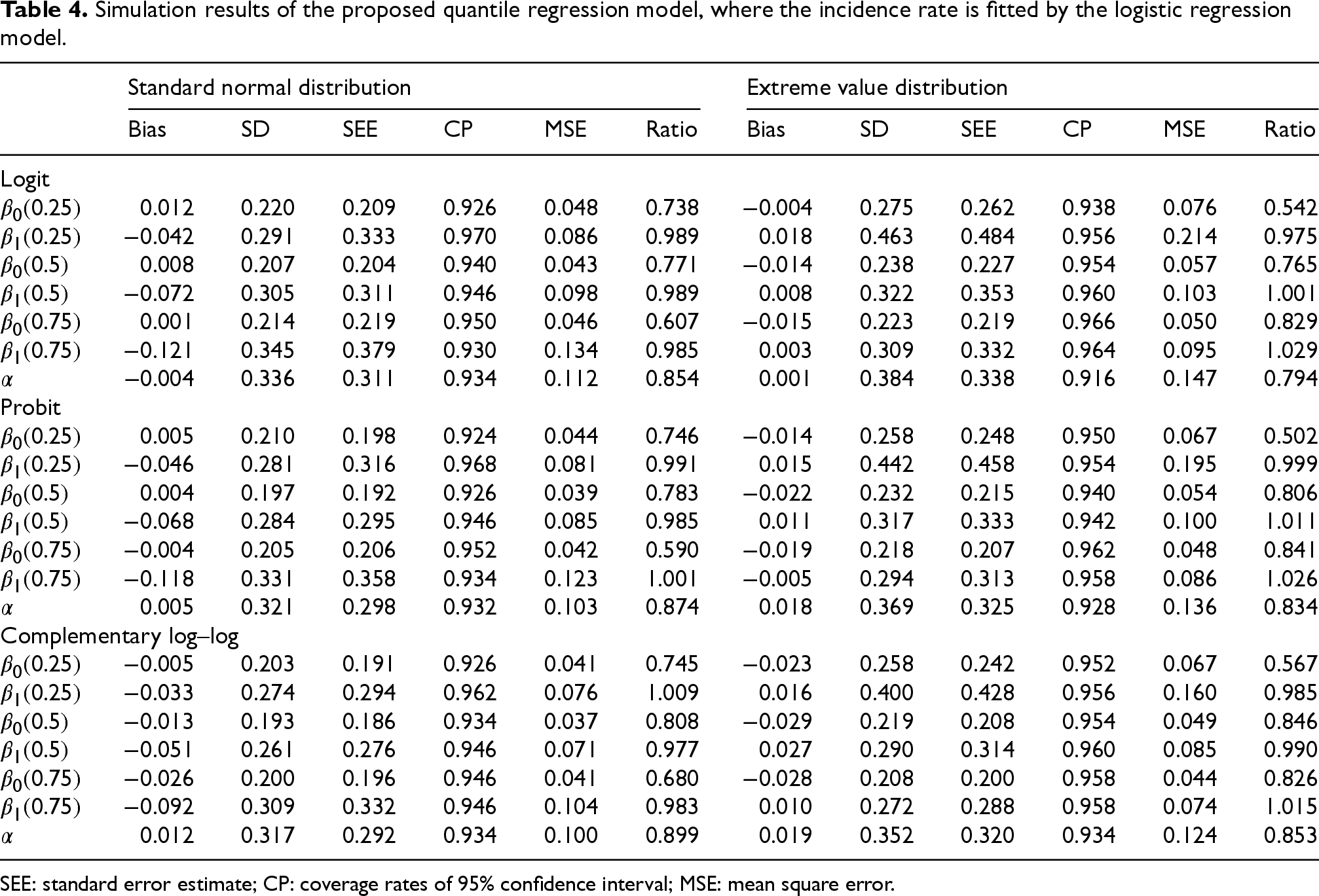
We further investigate the performance of the estimates of the partially functional covariate effects proposed in Section 3.2 using the same simulated data in Section 4.1. Under both settings, it is known that is constant, and we will treat it as in (7) and use the method in Section 3.2 to estimate , , and on the interval . We will compare the estimates with the fully functional covariate effect estimates from the method in Section 3.1. Since the estimates for are unchanged, we are only interested in the estimates of and . Table 4 shows the biases, SDs, SEEs, CPs, and MSEs of the estimates from the method in Section 3.2. The gain in efficiency by taking the homogeneous effect information of into account is demonstrated in the table by the ratios of the MSEs of and to those of and , and the ratios of the MSEs of to the MSEs of , where estimated via the fully functional covariate effects model.
Simulation results of the proposed quantile regression model, where the incidence rate is fitted by the logistic regression model.
Standard normal distribution
Extreme value distribution
Bias
SD
SEE
CP
MSE
Ratio
Bias
SD
SEE
CP
MSE
Ratio
Logit
0.012
0.220
0.209
0.926
0.048
0.738
−0.004
0.275
0.262
0.938
0.076
0.542
−0.042
0.291
0.333
0.970
0.086
0.989
0.018
0.463
0.484
0.956
0.214
0.975
0.008
0.207
0.204
0.940
0.043
0.771
−0.014
0.238
0.227
0.954
0.057
0.765
−0.072
0.305
0.311
0.946
0.098
0.989
0.008
0.322
0.353
0.960
0.103
1.001
0.001
0.214
0.219
0.950
0.046
0.607
−0.015
0.223
0.219
0.966
0.050
0.829
−0.121
0.345
0.379
0.930
0.134
0.985
0.003
0.309
0.332
0.964
0.095
1.029
−0.004
0.336
0.311
0.934
0.112
0.854
0.001
0.384
0.338
0.916
0.147
0.794
Probit
0.005
0.210
0.198
0.924
0.044
0.746
−0.014
0.258
0.248
0.950
0.067
0.502
−0.046
0.281
0.316
0.968
0.081
0.991
0.015
0.442
0.458
0.954
0.195
0.999
0.004
0.197
0.192
0.926
0.039
0.783
−0.022
0.232
0.215
0.940
0.054
0.806
−0.068
0.284
0.295
0.946
0.085
0.985
0.011
0.317
0.333
0.942
0.100
1.011
−0.004
0.205
0.206
0.952
0.042
0.590
−0.019
0.218
0.207
0.962
0.048
0.841
−0.118
0.331
0.358
0.934
0.123
1.001
−0.005
0.294
0.313
0.958
0.086
1.026
0.005
0.321
0.298
0.932
0.103
0.874
0.018
0.369
0.325
0.928
0.136
0.834
Complementary log–log
−0.005
0.203
0.191
0.926
0.041
0.745
−0.023
0.258
0.242
0.952
0.067
0.567
−0.033
0.274
0.294
0.962
0.076
1.009
0.016
0.400
0.428
0.956
0.160
0.985
−0.013
0.193
0.186
0.934
0.037
0.808
−0.029
0.219
0.208
0.954
0.049
0.846
−0.051
0.261
0.276
0.946
0.071
0.977
0.027
0.290
0.314
0.960
0.085
0.990
−0.026
0.200
0.196
0.946
0.041
0.680
−0.028
0.208
0.200
0.958
0.044
0.826
−0.092
0.309
0.332
0.946
0.104
0.983
0.010
0.272
0.288
0.958
0.074
1.015
0.012
0.317
0.292
0.934
0.100
0.899
0.019
0.352
0.320
0.934
0.124
0.853
SEE: standard error estimate; CP: coverage rates of 95% confidence interval; MSE: mean square error.
The results in the table show that the performance of the proposed estimation method is satisfactory: the biases are small, the SDs are similar to the SEEs, and the coverage probabilities are close to the nominal level. All the ratios in the estimation of and are between 0.502 and 1.03, indicating that taking the constant effect into account produces efficiency gain in estimating parameters in the latency part for most of the parameters. It is interesting to see that all the MSE ratios for are between 0.79 and 0.90. It indicates that a substantial efficiency gain is achieved by incorporating the information of quantile-invariant effects in the estimating procedure when compared to a naive method by averaging the estimate over .
Application to lung cancer data
As an illustration, we apply the proposed method to the data from the lung cancer study described in Section 1. The study involved 280 patients with lung cancer, and the event of interest is death due to lung cancer. The censoring rate is 64%. There were three covariates: tumor histology (172 patients with adenocarcinoma encoded as 1 and 108 with squamous cell carcinoma encoded as 0), sex (147 females encoded as 1 and 133 males encoded as 0), and age standardized with mean zero and variance 1.
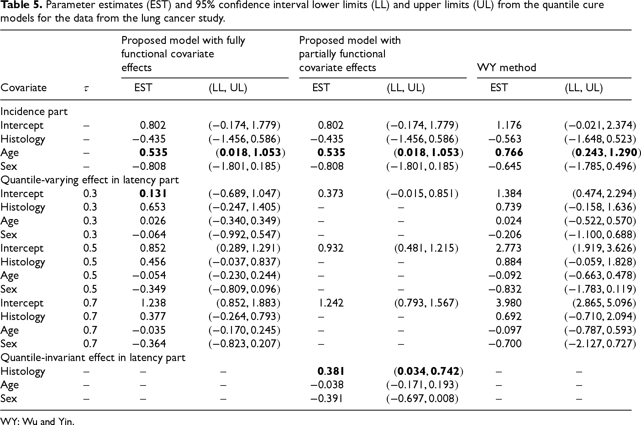
We are interested in examining the effects of histology, age, and sex using the quantile cure model and the estimation methods proposed in Sections 2 and 3. We first analyze the data by using the quantile cure model with fully functional covariate effects specified in (1) and (2) with the proposed estimation method, where includes histology, age, sex, and the intercept. We found no evidence to believe that the censoring time is associated with any of the covariates (see details in Section F in the Supplemental materials). Thus, in the proposed estimation method is estimated by the Kaplan–Meier estimator. The estimates and their 95% confidence intervals of the covariate effects in the logistic regression and the functional covariate effects at , 0.5, 0.7 are shown in the left columns of Table 5. The confidence intervals are obtained using weighted bootstrap samples. To make the comparison easier, we also show the results from the WY method in the right columns of Table 5. Age is the only variable reaching the 5% significance level in the incidence part from the proposed model, indicating that older patients have a lower chance of being cured than younger patients, which is consistent with the finding from the WY method, although the effect is smaller in the former than the latter.
Parameter estimates (EST) and 95% confidence interval lower limits (LL) and upper limits (UL) from the quantile cure models for the data from the lung cancer study.
Proposed model with fully functional covariate effects
Proposed model with partially functional covariate effects
WY method
Covariate
EST
(LL, UL)
EST
(LL, UL)
EST
(LL, UL)
Incidence part
Intercept
–
0.802
(−0.174, 1.779)
0.802
(−0.174, 1.779)
1.176
(−0.021, 2.374)
Histology
–
−0.435
(−1.456, 0.586)
−0.435
(−1.456, 0.586)
−0.563
(−1.648, 0.523)
Age
–
0.535
(0.018, 1.053)
0.535
(0.018, 1.053)
0.766
(0.243, 1.290)
Sex
–
−0.808
(−1.801, 0.185)
−0.808
(−1.801, 0.185)
−0.645
(−1.785, 0.496)
Quantile-varying effect in latency part
Intercept
0.3
0.131
(−0.689, 1.047)
0.373
(−0.015, 0.851)
1.384
(0.474, 2.294)
Histology
0.3
0.653
(−0.247, 1.405)
–
–
0.739
(−0.158, 1.636)
Age
0.3
0.026
(−0.340, 0.349)
–
–
0.024
(−0.522, 0.570)
Sex
0.3
−0.064
(−0.992, 0.547)
–
–
−0.206
(−1.100, 0.688)
Intercept
0.5
0.852
(0.289, 1.291)
0.932
(0.481, 1.215)
2.773
(1.919, 3.626)
Histology
0.5
0.456
(−0.037, 0.837)
–
–
0.884
(−0.059, 1.828)
Age
0.5
−0.054
(−0.230, 0.244)
–
–
−0.092
(−0.663, 0.478)
Sex
0.5
−0.349
(−0.809, 0.096)
–
–
−0.832
(−1.783, 0.119)
Intercept
0.7
1.238
(0.852, 1.883)
1.242
(0.793, 1.567)
3.980
(2.865, 5.096)
Histology
0.7
0.377
(−0.264, 0.793)
–
–
0.692
(−0.710, 2.094)
Age
0.7
−0.035
(−0.170, 0.245)
–
–
−0.097
(−0.787, 0.593)
Sex
0.7
−0.364
(−0.823, 0.207)
–
–
−0.700
(−2.127, 0.727)
Quantile-invariant effect in latency part
Histology
–
–
–
0.381
(0.034, 0.742)
–
–
Age
–
–
–
−0.038
(−0.171, 0.193)
–
–
Sex
–
–
–
−0.391
(−0.697, 0.008)
–
–
WY: Wu and Yin.
For the latency part, none of these three estimated quantile effects reaches the significant level from the fully functional covariate effect model by the proposed and the WY methods. To illustrate the functional effects of the covariates, we estimate the functional effects using the proposed method for with an equally spaced grid . Their estimates and the corresponding 95% confidence intervals are drawn in Figure 1. The results indicate that none of them reaches the significant level over the range, a similar conclusion as in the WY method. However, we can see that the estimated functional effects of histology, age, and sex over the quantile range appear to be constant, that is, homogeneous effects. As discussed in Section 3.3, an interesting question is whether or not these covariate effects are significantly quantile-varying on , and hence we apply the test in (12) to test the significance. The hypotheses and the test statistic for each of the three variables are given in (11). With , the -values of the test are 0.65, 0.75, and 0.68 for histology, age, and sex, respectively. Thus, we do not have strong evidence to reject the homogeneous quantile effects on . We also conducted the same testing with and obtained the same conclusion. Hence, it is interesting to consider the quantile regression (7) with partially functional covariate effects on , where only contains the intercept and contains histology, age, and sex. The estimates and their 95% confidence intervals from this model are shown in the middle columns of Table 5. The results demonstrate that histology has a significant effect on the distribution of , and uncured patients with adenocarcinoma have 46% () longer survival times than those uncured patients with squamous cell carcinoma. The results also demonstrate the efficiency gained by considering the partially functional covariate effects over the fully functional covariate effects when the former is adequate for the data. It is worth noting that the fitted model (7) with only an intercept in resembles the AFT mixture cure model,21,22 which was considered for this dataset by Wu and Yin3 (results are omitted here to save space). However, an important difference between the two models is that the quantile-invariant effects in the proposed model are for while the quantile-invariant effects in the AFT mixture cure model are for . Thus, it is not unexpected to find that, unlike the proposed model, the AFT mixture cure model does not show any significant effects in either of the two parts of the model.
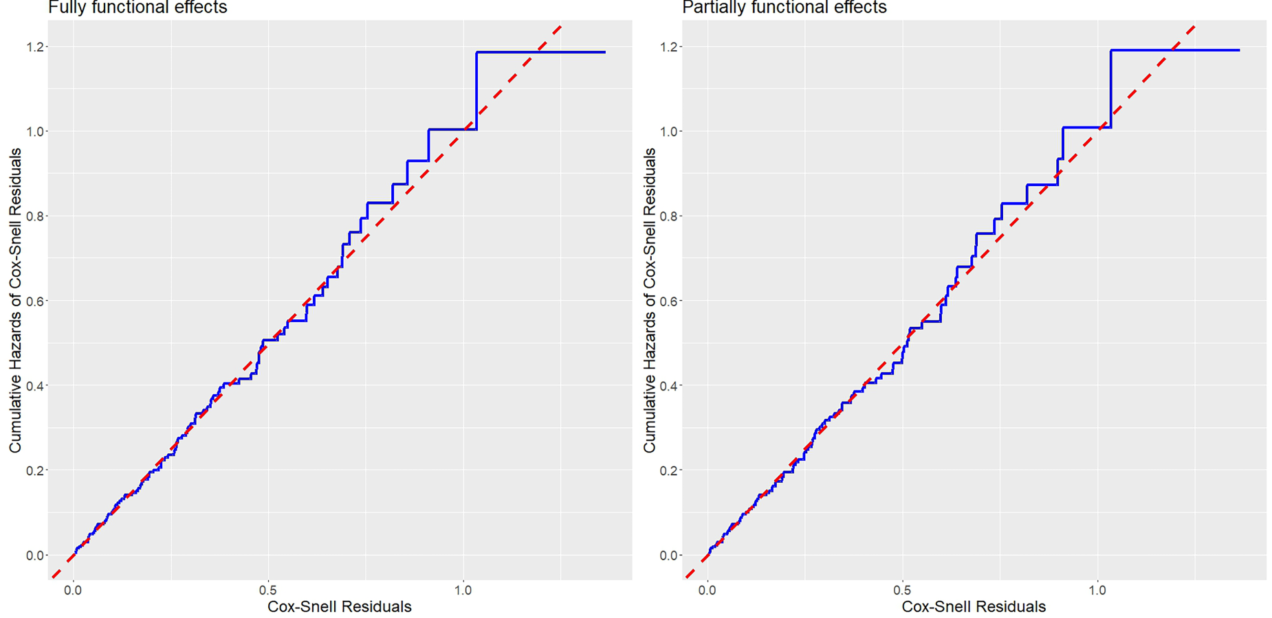
We also checked the fit of the proposed models using the proposed Cox–Snell residuals in Section 3. The Cox–Snell residual plots displayed in Figure 2 show that the proposed quantile mixture cure models with fully and partially functional covariate effects fit the data well, and there is no substantial departure from the line.
The Cox–Snell residual plots for the proposed cure models with fully (left) and partially (right) functional covariate effects on the quantiles of time to lung cancer death.
We also conducted a sensitivity analysis to investigate the robustness of the results to the choice of the interval . We considered intervals with 0.2, 0.25, and 0.3 as and 0.6, 0.65, 0.7, 0.75, and 0.8 as . We found that the results of the homogeneous test (12) of the three variables are robust to the changes in and . That is, the three variables do not show significant quantile-varying effects in any of the intervals considered. When the variables are included in the model with quantile-invariant effects in the intervals, the effects of the variables in the model also demonstrate considerable robustness to the changes in and . The insignificance of age and sex remains unchanged. The significance of the effect of histology may change sometimes with the lower bound of the 95% confidence interval slightly below zero. This is not unexpected given that the reported lower bound for histology in Table 5 is very close to 0.
Discussion
In this article, we considered a new mixture cure model, where a local quantile regression is used to model covariate effects at a specific quantile level or with partially functional covariate effects on a range of quantiles in the latency part of the cure model. The parameters in the incidence and latency parts are estimated separately, and thus, inference of each part is robust to the model misspecification of the other part. The large sample properties of the proposed estimators are established. The proposed approach is easy to implement and computationally more efficient than the existing methods. For the cure model with fully functional covariate effects, a test for the presence of quantile-invariant covariate effects is developed, which will facilitate investigators to select covariates for a parsimonious partially functional covariate effects model in the latency part when the fully functional covariate effects model is unnecessary.
The proposed quantile cure model with partially functional covariate effects is not limited to the same interval for all quantile-invariant effects. For example, consider the following quantile model in the latency part over : , where and , or the following model: , where , and are completely different from . Both models can be estimated straightforwardly using the proposed estimation method.
One crucial concern for the fully and partially functional covariate effects model in the latency part is the linearity assumption on a quantile range. A formal lack-of-fit test for assessing the linearity over the range needs to be established. Moreover, the range of quantiles also needs to be specified. Our additional simulation studies reveal that the inference can be improved by enlarging the subinterval . It is expected that the larger the subinterval , the more information that data can provide, and the higher efficiency and more accurate inference can be achieved in the estimation. In the current article, the subinterval is determined by a visual inspection of the fully functional covariate effect estimates like Figure 1.
For the quantile regression in the latency part, it is worth mentioning the differences between ours with other existing models/methods in the literature. The proposed cure model with partially functional covariate effects allows quantile-invariant effects for some covariates on a range of quantiles, while the AFT cure model assumes that all covariates have quantile-invariant effects for all in (0, 1). The partially functional covariate effects on the latency in the proposed method are also different from those of Qian and Peng9 in that the latter requires a strong global linearity assumption for all covariate effects at all quantile levels. Our model can be viewed as an extension of the model in Qian and Peng9 by relaxing the global linearity assumption. Furthermore, in contrast to the model of Chu and Sit10 that requires all covariate effects to be quantile invariant over the range of quantiles, our partially functional covariate effects model allows the effects of some covariates to be quantile-invariant while others to be quantile-varying.
A feature of the proposed method is that the estimating equations (6), (8), and (9) use the IPCW approach to estimate the parameters in the latency part based on uncensored subjects. The approach relies on a correctly specified model for the censoring time. Hence, it is important to conduct model diagnosis to ensure the appropriateness of the model. Gorfine et al.23 considered an augmented IPCW method to estimate a quantile regression model for right-censored data without a cured fraction. This method is doubly robust in the sense that it yields consistent estimates if either the censoring model or the model for the complete-data distribution is correctly specified. Extending the proposed method to a doubly robust estimation method to potentially achieve better efficiency is an important direction and warrants further investigation in future work.
Although we considered different link functions for the incidence part of the model, they may not be sufficient to capture the complex relationship between covariates and the cure probability. A further study is needed to relax the parametric assumptions in the proposed model. Machine learning methods have been considered recently in estimating cure models,24 such as the support vector machine,25 neural network,26 and gradient boosting decision trees.27 The machine learning methods can capture more complex covariate effects and tend to be more flexible than the model considered in this paper. Exploring machine learning methods for the proposed model is beyond the scope of this paper, and it will be investigated in future research.
Supplemental Material
sj-pdf-1-smm-10.1177_09622802261445414 - Supplemental material for A quantile cure model with partially functional covariate effects
Supplemental material, sj-pdf-1-smm-10.1177_09622802261445414 for A quantile cure model with partially functional covariate effects by Chyong-Mei Chen and Yingwei Peng in Statistical Methods in Medical Research
Supplemental Material
sj-zip-2-smm-10.1177_09622802261445414 - Supplemental material for A quantile cure model with partially functional covariate effects
Supplemental material, sj-zip-2-smm-10.1177_09622802261445414 for A quantile cure model with partially functional covariate effects by Chyong-Mei Chen and Yingwei Peng in Statistical Methods in Medical Research
Footnotes
ORCID iDs
Chyong-Mei Chen
Yingwei Peng
Funding
The authors disclosed receipt of the following financial support for the research, authorship, and/or publication of this article: The work of Yingwei Peng is partially supported by a research grant from the Natural Sciences and Engineering Research Council of Canada.
Declaration of conflicting interests
The authors declared no potential conflicts of interest with respect to the research, authorship, and/or publication of this article.
Supplemental material
Supplemental material for this article is available online.
References
1.
CoxDR. Regression models and life-tables. J R Stat Soc B1972; 34: 187–220.
2.
WeiLJ. The accelerated failure time model: a useful alternative to the Cox regression model in survival analysis. Stat Med1992; 11: 1871–1879.
3.
WuYYinG. Multiple imputation for cure rate quantile regression with censored data. Biometrics2017; 73: 94–103.
4.
PengLHuangY. Survival analysis with quantile regression models. J Am Stat Assoc2008; 103: 637–649.
5.
WuYYinG. Cure rate quantile regression for censored data with a survival fraction. J Am Stat Assoc2013; 108: 1517–1531.
6.
WangHJWangL. Locally weighted censored quantile regression. J Am Stat Assoc2009; 104: 1117–1128.
7.
NarisettyNKoenkerR. Censored quantile regression survival models with a cure proportion. J Econom2022; 226: 192–203.
8.
YangXNarisettyNNHeX. A new approach to censored quantile regression estimation. J Comput Graph Stat2018; 27: 417–425.
ChuCWSitT. Censored interquantile regression model with time-dependent covariates. J Am Stat Assoc2023; 119: 1592–1603.
11.
MiaoRSunLTianG-L. Transformed linear quantile regression with censored survival data. Stat Interface2016; 9: 131–139.
12.
ChenC-MShenP-SLinC-C, et al.Semiparametric mixture cure model analysis with competing risks data: application to vascular access thrombosis data. Stat Med2020; 39: 4086–4099.
13.
PengLFineJP. Competing risks quantile regression. J Am Stat Assoc2009; 104: 1440–1453.
14.
BeranR. Nonparametric regression with randomly censored survival data. Technical report. Berkeley, CA: University of California, 1981.
15.
MallerRAZhouX. Survival analysis with long-term survivors. New York, NY: John Wiley & Son Ltd, 1996.
ShaoJTuD. The jackknife and bootstrap. New York, NY: Springer Science & Business Media, 2012.
20.
PengYTaylorJMG. Residual-based model diagnosis methods for mixture cure models. Biometrics2017; 73: 495–505.
21.
ZhangJPengY. A new estimation method for the semiparametric accelerated failure time mixture cure model. Stat Med2007; 26: 3157–3171.
22.
LuW. Efficient estimation for an accelerated failure time model with a cure fraction. Stat Sin2010; 20: 661–674.
23.
GorfineMGoldbergYRitovY. A quantile regression model for failure-time data with time-dependent covariates. Biostatistics2017; 18: 132–146.
24.
EzquerroACancelaBLópez-ChedaA. On the reliability of machine learning models for survival analysis when cure is a possibility. Mathematics2023 Oct; 11: 4150.
25.
LiPPengYJiangP, et al.A support vector machine based semiparametric mixture cure model. Comput Stat2020; 35: 931–945.
26.
AselisewineWPalS. A neural network integrated accelerated failure time-based mixture cure model. Stat Comput2025; 35: 134.
27.
ZhengJLiPPengY. A gradient boosting decision tree based estimation method for the mixture cure model. J Appl Stat2026; 53: 484–509.
Supplementary Material
Please find the following supplemental material available below.
For Open Access articles published under a Creative Commons License, all supplemental material carries the same license as the article it is associated with.
For non-Open Access articles published, all supplemental material carries a non-exclusive license, and permission requests for re-use of supplemental material or any part of supplemental material shall be sent directly to the copyright owner as specified in the copyright notice associated with the article.