Comparison of partial least squares regression,least squares support vector machines,and Gaussian process regression for a near infrared calibration

Abstract

This paper investigates the use of least squares support vector machines and Gaussian process regression for multivariate spectroscopic calibration. The performances of these two non-linear regression models are assessed and compared to the traditional linear regression model, partial least squares regression on an agricultural example. The non linear models, least squares support vector machines, and Gaussian process regression, showed enhanced generalization ability, especially in maintaining homogeneous prediction accuracy over the range. The two non-linear models generally have similar prediction performance, but showed different features in some situations, especially when the size of the training set varies. This is due to fundamental differences in fitting criteria between these models.

Keywords

Near-infrared spectroscopy multivariate calibration partial least squares regression least squares support vector machines Gaussian process regression

Background

The problem of interest is the prediction of the concentration of a chemical constituent in a sample from its near-infrared (NIR) spectrum. A set of calibration samples is used to learn the quantitative relationship between the constituent concentration and NIR absorption spectrum. In general, spectral data sets are high-dimensional and require dimensional reduction. Traditional linear regression methods (including principal component regression (PCR) and partial least squares regression (PLSR)) first transfer raw spectral data into latent variables to reduce dimensionality of regressors, and then directly implement multiple linear regression on latent variables. These methods perform reasonably well in most practical applications. However, in some cases, e.g. when predictions are required over a large range so that nonlinearity occurs, linear models fail to keep their accuracy across the range. Non-linear regression models are then relevant. Popular non-linear models include support vector machines (SVMs), artificial neural networks (ANNs), and Gaussian process regression (GPR). Previous studies have shown that SVMs¹ and GPR² can be applied to multivariate spectroscopic calibration. Numerous feasibility studies have proven SVM is a very powerful tool on spectroscopic analysis, such as identification of teas,³ quantification of milk powder,⁴ classification of colonic tissues,⁵ and quantitative calibration on tobacco.⁶ GPR is a relatively new method for spectroscopic calibration, and previous studies have shown its superiority on modeling instrumental systematics,⁷ imaging spectroscopic analysis,⁸ and variable selection for calibration.⁹ A comparison research also indicated that SVMs outperformed PLS on some validation tests.¹⁰ In this article, least squares support vector machines (LS-SVMs) and GPR are further studied. Their performances on a NIR spectroscopic calibration are compared to the traditional linear regression method, PLSR, on several aspects, including global error, local prediction behavior, and learning efficiency.

Theory

All the models mentioned here are based on learning a prediction rule on an observed data set, which is also called calibration set. However, these models have different learning and prediction strategies. They can be divided into two categories according to the way they make predictions: one, called variable space-based prediction, calculates the correlation coefficients between each of the variables and the target analyte; the other, called sample space-based prediction, ignores individual variable but focuses on affinity and dissimilarity between the samples. PLSR is the first type and the non-linear methods investigated here, LS-SVMs and GPR, are the second type.

Partial least squares regression

PLSR is a predictive two-block regression method based on estimated latent variables, initially developed by Wold et al.¹¹ and first applied to NIR data by Martens and Jensen.¹² The purpose of PLSR is to predict the property of interest y from observed NIR spectra $x = (x_{k}, k = 1, 2 \dots K)$ . This is achieved by a linear predictor

\overset{\land}{y} = b_{0} + \sum_{k = 1}^{K} b_{k} x_{k}

(1)

where b₀ is the offset and b_k are regression coefficients calculated by the PLSR algorithm. Notice that for each observed spectrum

x

the dimensionality K can be very high (typically hundreds of wavelengths in NIR spectra), and a regression model on all variables will be extremely complicated and noisy, so raw spectral data sets usually need dimension reduction before being regressed. As a result, multiple linear regression is actually performed on a set of PLS factors. These factors are calculated and taken out from the data set sequentially.¹³ Considering a training data set with I observations

y = (y_{i}, i = 1, 2 \dots I) T

, the corresponding spectra

X = (x_{ik}, i = 1, 2 \dots I; k = 1, 2 \dots K)

are taken as sum of several orthogonalized PLS factors, indexed by

a = 1, 2 \dots A

X

and

y

are first mean centered, producing

X_{0}

and

y_{0}

X_{0} = X - 1 \bar{x} T

y_{0} = y - 1 \bar{y} T

(2)

The residual on $X$ and $y$ after elimination of the a^th factor are termed $X_{a}$ and $y_{a}$ . The loading weight vector for the $a th$ PLS factor $w_{a}$ can be calculated by making use of the variability in $y_{a - 1}$ , formulated as

X_{a - 1} = y_{a - 1} w_{a}^{T} + X_{a}

(3)

under the condition that

w_{a}^{T} w_{a} = 1

. Minimize

X_{a}

with respect to

w_{a}

, the solution is given by

{\overset{\land}{w}}_{a} = c X_{a - 1}^{T} y_{a - 1}

(4)

Correspondingly, the PLS score $t_{a}$ for the a^th factor can be determined as the projection of $X_{a - 1}$ on ${\overset{\land}{w}}_{a}$

{\overset{\land}{t}}_{a} = X_{a - 1} {\overset{\land}{w}}_{a}

(5)

Loading vectors $p_{a}$ and q_a can be estimated by regressing $X_{a - 1}$ and $y_{a - 1}$ on ${\overset{\land}{t}}_{a}$

X_{a - 1} = {\overset{\land}{t}}_{a} p_{a}^{T} + X_{a} y_{a - 1} = {\overset{\land}{t}}_{a} q_{a} + y_{a}

(6)

Finally, the regressors described in equation (1) can be defined by

\overset{\land}{b} = \overset{\land}{W} (\overset{\land}{P} T \overset{\land}{W}) - 1 \overset{\land}{q}

(7)

and the offset

{\overset{\land}{b}}_{0}

is given by

{\overset{\land}{b}}_{0} = \bar{y} - \bar{x} T \overset{\land}{b}

(8)

Least squares support vector machines

PLSR is normally considered as one of the most powerful high-dimensional linear regression methods. However, the performance of PLSR is sometimes limited due to a non-linear relationship between the input variables and the response. In order to extend the regression method to a non-linear framework, new variables representing non-linearity need to be introduced. This can be achieved by mapping the input data into a higher dimensional feature space through a transformation $φ (\cdot) : ℝ k \to ℝ k_{h}$ . This mapping process is done by a linear basis expansion in the input variables, including non-linear transformations and combinations of the basis variables. The introduced non-linear feature space potentially has infinite dimension. Function estimation $\overset{\land}{y} (x)$ on an observed sample $x$ is then performed as follows

\overset{\land}{y} (x) = w T φ (x) + b

(9)

where b is the offset term and

w

is a vector of regression coefficients in the non-linear feature space. Such a coefficient vector also has potentially infinite dimensions. Given a training set with known responses

y = (y_{i}, i = 1, 2 \dots I) T

and corresponding observations

X = (x_{ik}, i = 1, 2 \dots I; k = 1, 2 \dots K)

, one can easily construct a ridge regression cost function in feature space

L = \frac{1}{2} w T w + γ \frac{1}{2} \sum_{i = 1}^{I} (w T φ (x_{i}) + b - y_{i}) 2

(10)

where γ controls the regularization procedure, and is related to the signal to noise ratio in the measurements. The bigger the value of γ, the higher the signal to noise ratio, and the less the necessary shrinkage in the coefficients.

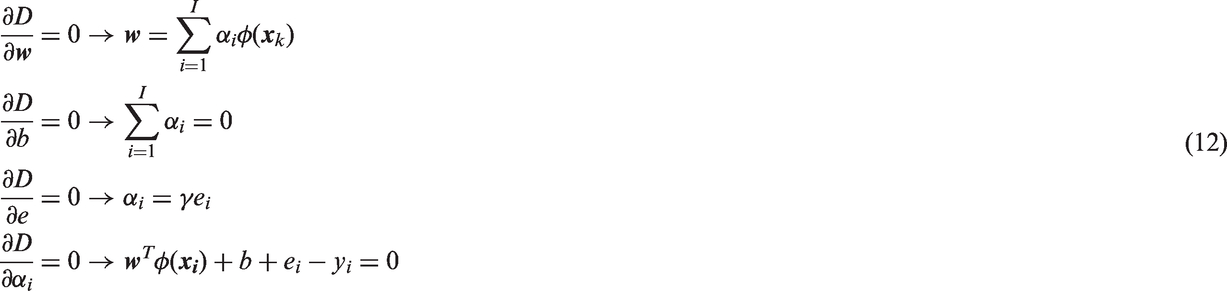
However, this problem is not solvable due to potentially infinite dimensionality. Instead we construct the Lagrange dual function¹⁴

D (w, b, e; α) = L - \sum_{i = 1}^{I} α_{i} w T φ (x i) + b + e_{i} - y_{i}

(11)

with Karush–Kuhn–Tucker conditions¹⁵

Substituting $w$ and e, the solution on $α$ and b can be expressed as

[0 1 T 1 Ω + I / I γ γ] b α = [0 y]

(13)

where

Ω

is the kernel function

Ω_{nm} = φ (x_{n}) T φ (x_{m}) = K (x_{n}, x_{m}) Ω = K (X, X) n, m = 1, 2 \dots I

(14)

In the following experiment only the radial basis function (RBF) kernel is considered, formulated as

K (x_{n}, x_{m}) = \exp (- \frac{∥ x_{n} - x_{m} ∥_{2}^{2}}{l 2})

(15)

The prediction for a new observation $x_{I + 1}$ can be expressed as

\overset{\land}{y} (x_{I + 1}) = \sum_{i = 1}^{I} α_{i} φ (x_{I + 1}) φ (x_{i}) + b = \sum_{i = 1}^{I} α_{i} K (x_{I + 1}, x_{i}) + b

(16)

Substituting $α$ with solution in equation (13), one can get following equation

\overset{\land}{y} (x_{I + 1}) = K (x_{I + 1}, X_{i}) [K (X, X) + I / I γ γ] - 1 [y - b \cdot 1] + b

(17)

Notice that only two free parameters $(γ, l)$ need to be tuned in the final target formulation. γ is influenced by the signal to noise ratio, and l, which is sometimes called length-scale in the input space, represents how sensitive $y$ is to changes in $X$ . When l is small, $y$ is very sensitive to variances in the input variables and thus can potentially produce precise predictions, but with a huge risk of over-fitting. When l is large, $y$ changes slowly, so predictions are less precise but more robust. These two free parameters can be tuned through cross-validation in training set to minimize the target loss function, for example, squared error loss as utilized here.

Gaussian process regression

A Gaussian process (GP) is a collection of random variables such that any finite subset exhibits a joint Gaussian distribution.¹⁶ First consider that an observation y_i in the calibration set $y = (y_{i}, i = 1, 2 \dots I) T$ consists of a true underlying function f_i, which is also called the latent function, and an additional Gaussian white noise $ε$

y_{i} = f_{i} + ε

(18)

Assume this Gaussian white noise has zero mean and precision of γ, then the probability distribution of the observations given the latent function can be described by a Gaussian likelihood function

P (y | f) = N (f, \frac{1}{γ} I)

(19)

There are many other possible likelihood functions for complicated relationship between latent function and observations, depending on the type of the noise, but in the following study only Gaussian likelihood is considered. The latent function described above is the target GP. Similar to mean and variance in a Gaussian distribution, a GP is fully defined by its mean function $M$ and covariance function $K_{GP}$ . Given a set of input variables $X = x_{1}, x_{2} \dots x_{I}$ , the latent function variable $f = f_{1}, f_{2} \dots f_{I}$ has a joint Gaussian distribution

P (f | X) = N (M, K_{GP} (X, X))

(20)

where

M

is the mean vector with the size of I and

K_{GP}

is a

I \times I

covariance matrix. Again, the RBF kernel function can be implemented here, as formulated in equation (15), but with an additional parameter

σ_{s}^{2}

to determine the signal level. The

(n, m)

^th element of

K_{GP} (X, X)

is formulated as

K_{GP} (x_{n}, x_{m}) = σ_{s}^{2} K (x_{n}, x_{m}) = σ_{s}^{2} \exp (- \frac{∥ x_{n} - x_{m} ∥_{2}^{2}}{l 2})

(21)

Normally, for notational and computational convenience, the mean function is set to $0$ , and this is appropriate if the response is mean centered. So equation (20) can be modified as

P (f | X) = N (0, K_{GP} (X, X))

(22)

Multiplying equation (22) with the likelihood function in equation (19), and integrating out $f$

P (y | X) = N (0, K_{GP} (X, X) + \frac{1}{γ} I)

(23)

Similarly to the other prediction models, the main interest is making predictions on new measurements based on the information from a training (calibration) data set $X = (x_{i}, i = 1, 2 \dots I)$ and $y = (y_{i}, i = 1, 2 \dots I) T$ . GPR assumes that the observation y has a joint Gaussian distribution with mean of 0 (after mean centered) and a covariance function given by $K_{GP} (X, X) + \frac{1}{γ} I$ . One can easily write down the marginal likelihood

P (y | 0, K_{GP} (X, X) + \frac{1}{γ} I) = (2 π) - \frac{I}{2} | K_{GP} (X, X) + \frac{1}{γ} I | - \frac{1}{2} \times exp (- \frac{1}{2} y T (K_{GP} (X, X) + \frac{1}{γ} I) - 1 y)

(24)

The three free parameters $γ, σ_{s}^{2}$ , and l in equation (23) can be tuned to maximize this marginal likelihood on the training set. This technique is sometimes called evidence maximization. Different from cross-validation in PLSR and LS-SVMs, evidence maximization uses the whole training set at one time, without dividing it into calibration and validation groups. More importantly, the optimization target is not to reduce the squared error loss function, which only depends on the point prediction. The likelihood is determined by both the mean and the covariance of posterior distribution. This also explains why an additional parameter $σ_{s}^{2}$ is needed in the GPR framework.

For prediction of a new observation $x_{I + 1}$ , we construct a set of $I + 1$ latent variables $f_{1}, f_{2} \dots f_{I}, f_{I + 1}$ with a joint zero mean Gaussian distribution and predefined covariance function

P (f_{1}, f_{2} \dots f_{I}, f_{I + 1}) = N (0, K_{GP} (X, X) K_{GP} (X, x_{I + 1}) K_{GP} (x_{I + 1}, X) σ_{s}^{2})

(25)

Taking into account the Gaussian noise $ε$ in $y$ , the joint Gaussian distribution of $y$ and $f_{I + 1}$ can be expressed as

P (f_{1}, f_{2} \dots f_{I}, f_{I + 1}) = N (0, K_{GP} (X, X) + \frac{1}{γ} I K_{GP} (X, x_{I + 1}) K_{GP} (x_{I + 1}, X) σ_{s}^{2})

(26)

The conditional probability $f_{I + 1} | X, y, x_{I + 1}$ has the expectation and variance of

mean ({\overset{\land}{f}}_{I + 1}) = K_{GP} (x_{I + 1}, X) [K_{GP} (X, X) + \frac{1}{γ} I] - 1 y var ({\overset{\land}{f}}_{I + 1}) = σ_{s}^{2} - K_{GP} (x_{I + 1}, X) [K_{GP} (X, X) + \frac{1}{γ} I] - 1 \times K_{GP} (X, x_{I + 1})

(27)

Compared with LS-SVMs, GPR not only gives a prediction mean for the new observation, but also provides a full probabilistic posterior distribution. This additional information is sometimes very useful, for example for outlier detection. However, since interpreting variance on predictions requires one more degree of freedom, it also increases the difficulty of tuning the hyper-parameters, especially when the training set is a small one.

Experiment

Three high-dimensional regression models (PLSR, LS-SVMs and GPR) were applied to the same NIR spectral data set. Their performances in prediction were presented and compared. All of the calculations were performed in Matlab R2014b (The MathWorks Inc, MA). PLSR was achieved with the Statistics and Machine Learning Toolbox; LS-SVM was realized with LS-SVMlab package;¹⁷ and GPR was calculated with GPML package.¹⁸

Sample composition

The data set consists of NIR spectra and corresponding target constituent concentration (nitrogen) from 1240 agricultural seeds. Images were recorded using a mercury–cadmium–telluride hyper-spectral camera and then post processing was used to average the spectral points over the seeds to produce a single spectrum per seed. For each spectrum there are 239 valid wavelengths in the NIR range, spanning from 993.0 nm to 2488.4 nm. The constituent content was then measured using a combustion-based chemical analysis.

Preprocessing

Several preprocessing methods were evaluated by cross-validation using the PLSR model. The combination of SNV + Savitzky-Golay derivative was implemented. Raw spectra were first preprocessed by standard normal variate (SNV), to remove constant offset and scatter effect by centering and rescaling individual spectrum, and then transformed with Savitzky-Golay 2 side points, second polynomial order fitting first derivative.

Randomization

The 1240 spectra were first randomly divided into two groups: group A (with 360 spectra) as calibration set and group B (with 880 spectra) as validation set. Figure 1 shows the density distribution, for nitrogen of one pair of randomized calibration and validation sets. All of the three regression methods were trained on the same calibration set first. Obtained models were then applied to predict nitrogen concentration in the validation set according to their spectra, and then compared to their true responses. This randomized test was performed five times in total. In each single test, the validation set was carefully kept away from optimizing the model, so error on the validation set can be seen as a good indicator of generalized prediction performance.

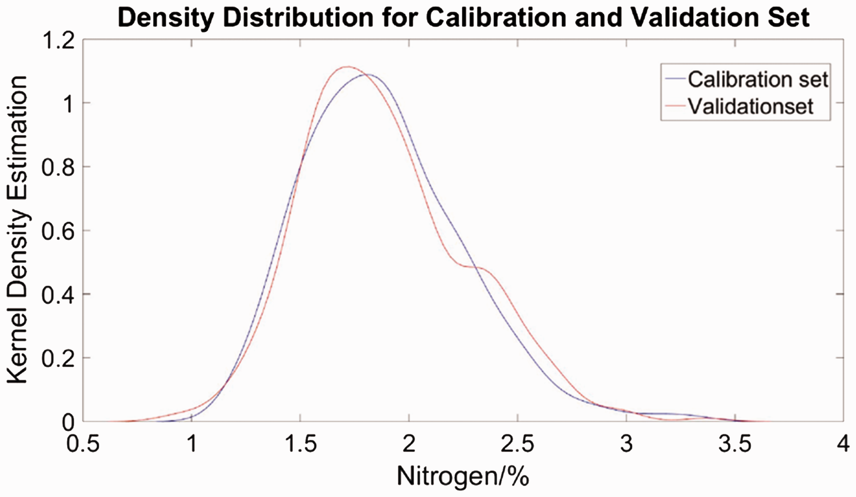
The three regression models were trained on calibration set as follows.

Partial least squares regression

As described in ‘Partial least squares regression’ section, there is only one free parameter in the PLSR model: the number of PLS factors used for prediction. Although higher order factors contain more detailed features from the variance of regressors, this is not necessarily correlated with the response (nitrogen concentration). Using higher order components will inevitably lead to a more complicated model, which may generalize less well. Cross-validation is very useful for choosing a reasonable highest order of PLS factor. An internal 10-fold cross-validation was performed on the PLSR model with different numbers of factors. Mean square error of cross-validation (MSECV) was taken as an indicator of the quality of the tested model.

Figure 2 shows RMSECV values for one randomized calibration set. This parameter selection process was separate from the test set, and was solely used for choosing the number of PLS factors. According to the result, cross-validation suggests using a PLSR model with 11 components. Notice in Figure 2 that 11 and 12 components had very close MSECV values (0.035% and 0.034% respectively) and 11 was adopted, because when two PLSR models have comparable performances, the simpler one is preferred.

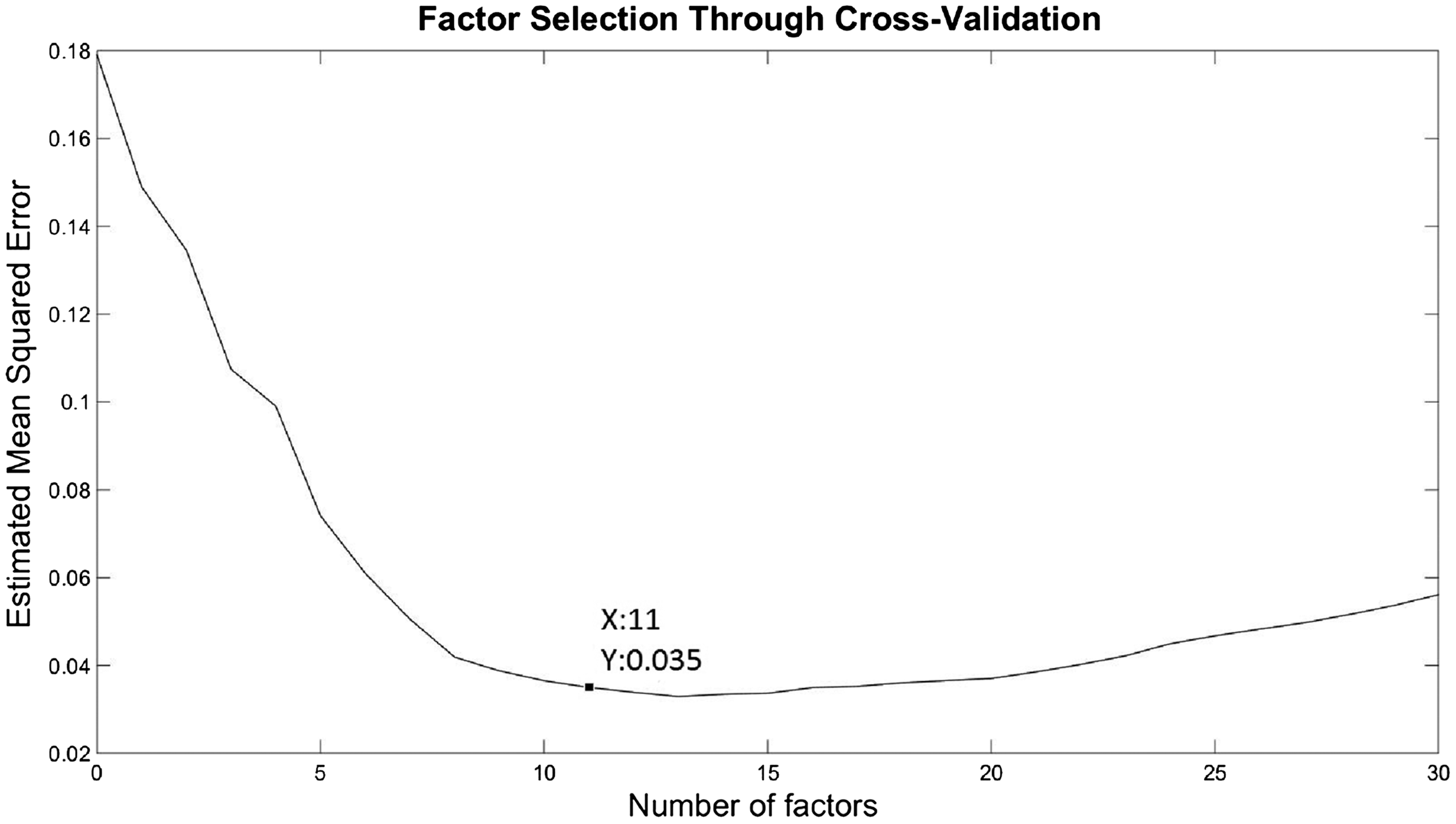
Least squares support vector machines

For the non-linear regression model LS-SVMs, there are two free hyper-parameters: γ, related to the strength of regularization term, and l, determining the length scale of the adopted RBF kernel. Both of these free parameters need to be tuned through the cross-validation process. Initial values of γ and l were decided by coupled-simulated annealing (CSA), a global optimization method composed of several distributed simulated annealing processes with coupled acceptance probability,¹⁹ to avoid very bad local minima. The two parameters were then tuned to minimize the squared error loss function $L_{γ, l} = \sum_{i = 1}^{I} ({\overset{\land}{y}}_{i} - y_{i}) 2$ with 10-fold cross-validation.

Gaussian process regression

A GP is fully defined by a mean function, covariance function and a likelihood function. The options for these three functions in the study are described as follows:

Mean function: In order to simplify the computational work, before GPR was carried out all the response was mean centered to 0 by taking out the offset. As a result, the mean function was set to $0$ .

Covariance function: RBF (with magnitude) was used as the covariance function in GPR, as described in equation (21). There are two hyper-parameters in this covariance function: isotropic length scale l and signal magnitude $σ_{s}^{2}$ .

Likelihood function: Assuming noise on observations has a Gaussian distribution, the Gaussian likelihood function was adopted here. Noise magnitude was specified by $1 / γ$ .

In total, there are three free parameters: $σ_{s}^{2}$ , l, and γ. All of them were optimized through evidence maximization using the training set, as described in ‘Gaussian process regression’ section. Notice that no initialization (like CSA in LS-SVMs) on the parameters was done before making inference on hyper-parameters, so potentially there was a very high risk of falling into multiple bad local optima. However, experimental results indicated that local optima were not a severe problem here, especially for large training set cases, because usually there is only one local optimum with a significantly higher marginal likelihood so it will be easy to reject all the other models.

Results

Comparing global RMSEV

As discussed in the previous section, the 1240 data points were randomly divided into two sets: calibration set with 360 samples and validation set with 880 samples. The calibration set and validation set were fully randomized and tested five times for each model. Since the predictions from all the models at each test were correlated because the validation set was a common one, errors in the laboratory measurements for the 880 samples contributed to all sets of prediction errors.²⁰ T test for paired samples can be utilized to calculate the true differences on biases and true ratio of root mean square error for validation (RMSEV).

Careful comparisons on biases and RMSEV between the three models were performed on five separate randomized tests. Results presented in Table 1 show RMSEV and biases for three models on each randomized validation set. Table 2 presents the 95% confidence intervals for the true difference in biases. Table 3 shows the 95% confidence intervals for the true ratio of RMSEV.

Table 1.

RMSEV and biases (%) for PLSR, LS-SVMs and GPR on each randomized validation set.

Index	PLS		LS-SVMs		GPR
Index	RMSEV	Bias	RMSEV	Bias	RMSEV	Bias
1	0.165	0.013	0.134	0.004	0.131	0.004
2	0.166	0.005	0.133	0.002	0.131	0.004
3	0.162	0.010	0.131	0.016	0.123	0.007
4	0.164	0.006	0.127	0.001	0.125	0.006
5	0.168	−0.010	0.126	−0.004	0.125	−0.002
Average	0.165	0.005	0.130	0.004	0.127	0.004

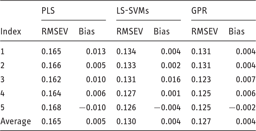
GPR: Gaussian process regression; LS-SVMs: least squares support vector machines; PLSR: partial least squares regression; RMSEV: root mean square error for validation.

Table 2.

The 95% confidence intervals for the true difference in biases (% nitrogen).

Index	PLS–LS-SVMs	PLS–GPR	LS-SVMs–GPR
1	(0.002,0.017)	(−0.002,0.036)	(−0.011,0.025)
2	(−0.003,0.024)	(−0.007,0.04)	(−0.013,0.024)
3	(−0.014,0.002)	(−0.014,0.036)	(0.006,0.040)
4	(−0.003,0.012)	(−0.007,0.03)	(0.006,0.040)
5	(−0.013,0.002)	(−0.031,0.008)	(−0.023,0.011)
Average	(−0.006,0.011)	(−0.012,0.030)	(−0.010,0.025)

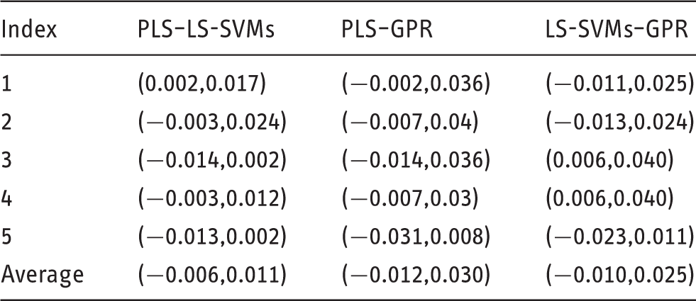
GPR: Gaussian process regression; LS-SVMs: least squares support vector machines; PLS: partial least square.

Table 3.

The 95% confidence intervals for the true ratio of RMSEV (% nitrogen).

Index	PLS / LS-SVMs	PLS / GPR	LS-SVMs / GPR
1	(1.171,1.283)	(1.198,1.311)	(0.994,1.045)
2	(1.176,1.302)	(1.202,1.324)	(0.996,1.045)
3	(1.190,1.308)	(1.266,1.380)	(1.021,1.089)
4	(1.236,1.352)	(1.253,1.374)	(0.990,1.039)
5	(1.274,1.392)	(1.294,1.404)	(0.991,1.033)
Average	(1.209,1.327)	(1.243,1.359)	(0.998,1.050)

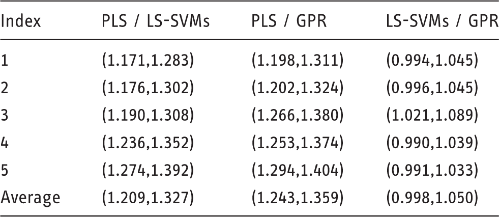
GPR: Gaussian process regression; LS-SVMs: least squares support vector machines; PLS: partial least square; RMSEV: root mean square error for validation.

Several important conclusions can be drawn from above results:

For all the randomization tests, there are steady and significant differences on the RMSEV between PLS/LS-SVMs and PLS/GPR. The LS-SVMs and GPR always out-performed PLSR in the sense of RMSEV. Averaged ratios of RMSEV were: PLSR/LS-SVMs = 1.270; PLSR/GPR = 1.300.

Randomized test 3 showed that the RMSEV and bias of LS-SVMs are significantly larger than GPR, but both the magnitudes of differences are very small. Other tests show no significant differences on RMSEV and bias. These results indicate that the two non-linear models are equivalent on predicting target response.

Most of the randomized tests showed no significant difference in biases between PLS, LS-SVMs and GPR; this is not a surprise since all the models were expected to be globally unbiased.

Local error behavior

The non-linear models performed better than the linear model in the sense of global error. In this section, predictive behaviors for the three models on each individual sample in the validation set are reported to help understand how linear and non-linear models differ over the whole range. One good way to visualize local error behavior is to plot predictions against their true observations on the whole validation set, as shown in Figure 3.

Predicted vs. observed for PLSR

Predicted vs. observed for LS-SVMs

Predicted vs. observed for GPR.

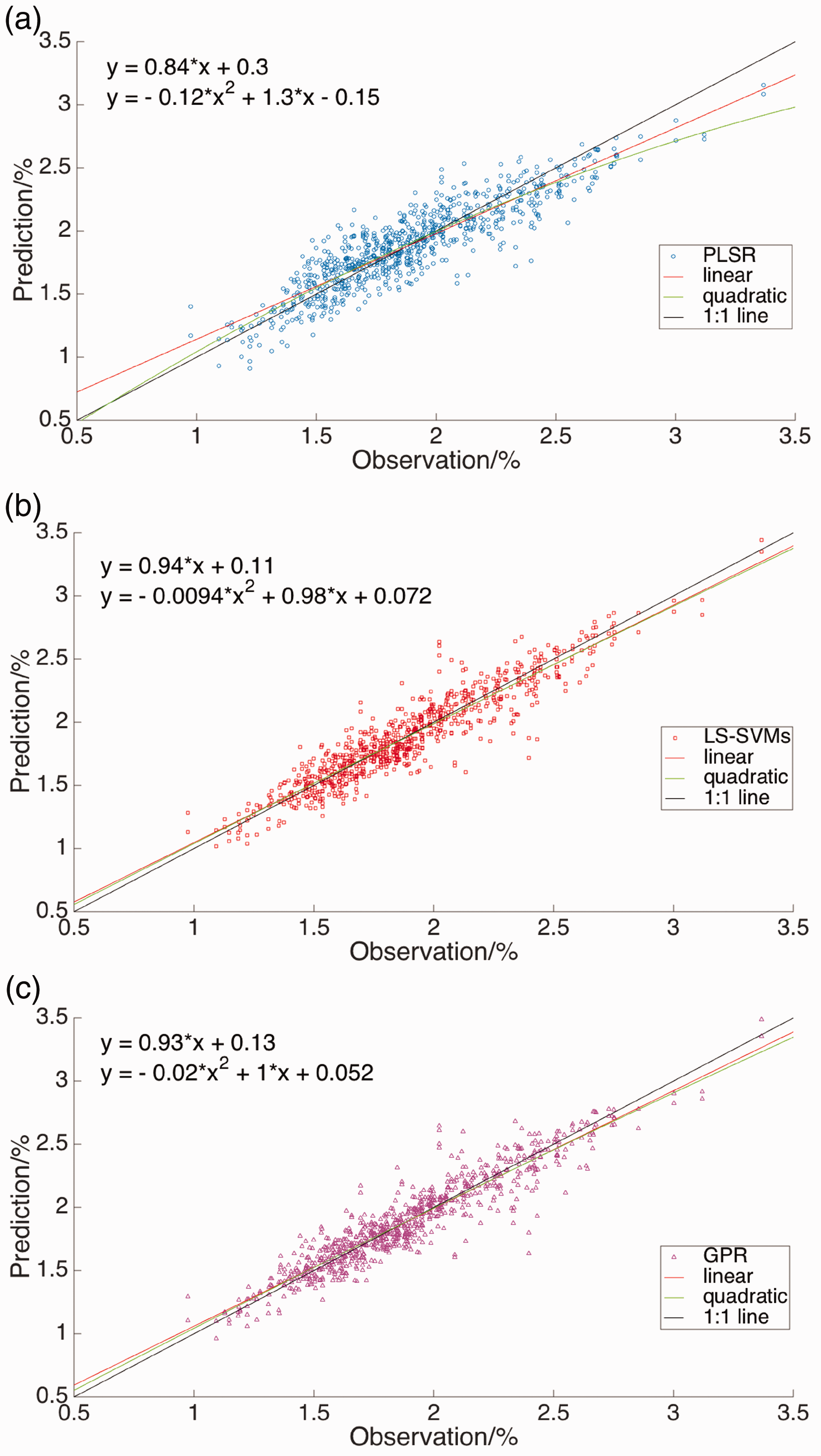
For PLSR, even though the performance was acceptable in the middle part of range (roughly 1.5–2.5%), predictions were heavily biased in the two tails from the regression line. There are two reasonable explanations:

The investigated constituent (nitrogen) concentration had an approximately linear impact on NIR spectra within a small range near the population mean, but non-linear effects become non-ignorable outside this linear range.

Prediction power for PLSR was limited. In order to minimize global error, PLSR will try to give best prediction in the center part, which accounts for the majority of the population. As a result, within this range linear correlation between observations and predictions was well maintained. The extreme samples are predicted less well, though this has a limited impact on the overall squared error cost function because there are far fewer of them (see Figure 1).

In contrast, the non-linear models (GPR for example here) had fairly consistent standard deviation from the regression line across the range. Non-linear biases at two tails were removed and predictions were then almost linearly related to the observations for all the samples in the validation set. The slope of regression line was also improved from 0.84 to 0.93 by using GPR. Considering any inverse calibration method implicitly uses population distribution in the training set as a prior, all the predictions are naturally shifted to the sample mean,²¹ in order to minimize global error. For non-linear models, since the fit was much better, this shrinkage to the mean was much less pronounced.

In order to quantitatively compare predictive performance of PLS, LS-SVMs, GPR on the low and high constituent ranges, predictions on the first 5% and the last 5% of the samples in the test set were calculated separately, ranked by their nitrogen concentration. Again, since all the comparisons were carried on a common validation set for each test, the same methods were used to see whether the differences on RMSEV and bias were significant, same as presented in ‘Comparing global RMSEV’ section. Detailed results on PLSR and GPR are shown in Table 4.

It can be seen, unsurprisingly, that GPR was significantly better than PLS everywhere across the range, in the sense of RMSEV. Especially, the ratio of RMSEV was further enlarged in the two tails.

There was no significant difference on the biases on the whole range, and both were very close to 0, because both the models are based on unbiased decision rules. However, there were significant differences on biases on low and high concentration range, and PLSR was, surprisingly, less biased on the first 5% of the samples. This is explained in Figure 4.

Table 4.

Comparison of PLSR and GPR on different % nitrogen ranges.^a

Model	Low (first 5%)		High (last 5%)		All
Model	RMSEV	Bias	RMSEV	Bias	RMSEV	Bias
PLSR	0.151	0.009	0.213	−0.156	0.160	0.013
GPR	0.108	0.020	0.160	−0.091	0.130	0.010
CI	(1.250,1.572)	(−0.037, −0.016)	(1.152,1.541)	(−0.094, −0.034)	(1.189,1.268)	(−0.004,0.011)

CI: confidence interval; GPR: Gaussian process regression; PLSR: partial least squares regression; RMSEV: root mean square error for validation.

Last row presents 95% confidence interval for the true difference of biases and true ratio of RMSEVs.

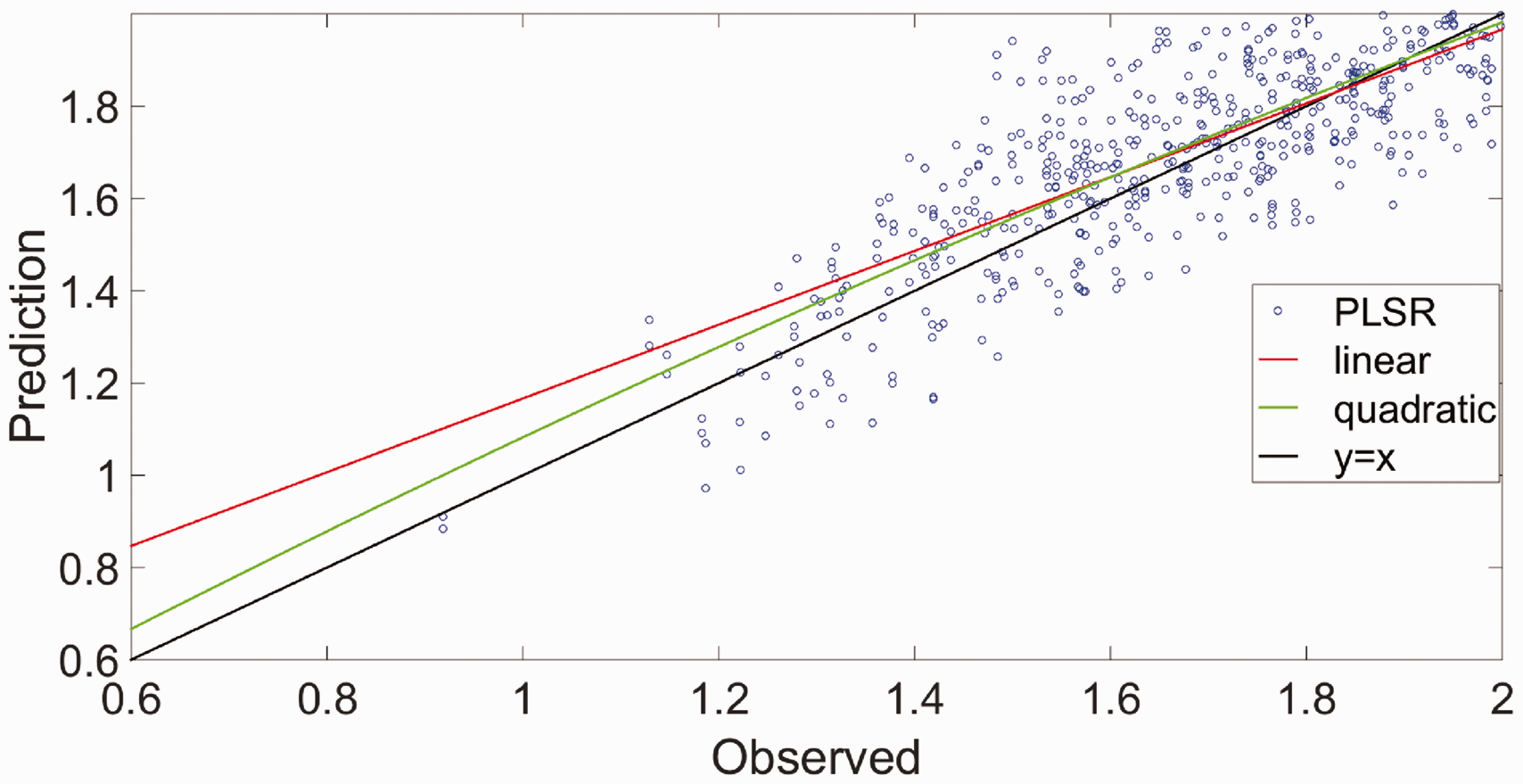
The red line is the regression line of prediction on observed data set. The y = x black line shows the shrinkage of the mean that occurs with PLSR. Because this shrinkage is in the same direction on the curvature of this end of the range, it actually reduces the bias of PLSR. In contrast, at the high end of the range, the shrinkage and curvature are in opposite directions, and PLSR has a very high bias compared to GPR.

Varying training set size

All the above analyses are conditional on a fixed size training set. A very important question is how fast each model learns with a growing training set. In practice, the reference measurement could be very expensive and time consuming. Sometimes there will not be sufficient training samples. Then it becomes desirable to understand how these different models perform with varying training set size. In Figure 5, global error on the validation set (RMSEV) is plotted against the number of samples in the training set. For each fixed size of training set, RMSEV is averaged over five randomized groupings of calibration and validation sets.

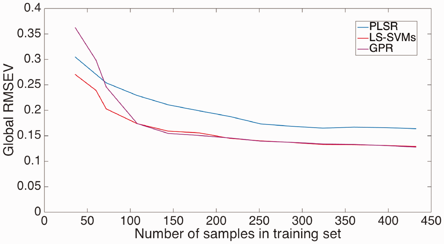
It can be observed that global errors for all the three models decreased when the training set size increased, and then gradually converged to their limits. However, they exhibited different learning speeds. LS-SVMs and PLSR had similar trends, except for a roughly constant offset on RMSEV between the two models. For GPR, when the training set size was small, the prediction power was extremely poor (a RMSEV of 0.38% is almost the width of population distribution in the validation set, so the GPR model gave almost homogeneous predictions despite the variation in the spectra), but the predicting power grew quickly with an increase in training set size, and soon became non-distinguishable from LS-SVMs.

This is the first time in this study when GPR and LS-SVMs exhibited significant difference in their predictive performance. Inevitably one wishes to ask a question: what are the differences between LS-SVMs and GPR? By comparing equation (17) and equation (27), it can be seen that predictions on a new measurement were effectively the same. The covariance function used in GPR was $K_{GP} = σ_{s}^{2} K$ , where $K$ is the kernel function used in LS-SVMs. If we scale $1 / 1 γ γ$ with the same multiplier $σ_{s}^{2}$ then this multiplier actually does not affect ${\bar{f}}_{I + 1}$ . By further setting the offset term b in LS-SVMs to 0, they had exactly the same form of prediction. This means, for an appropriate choice of hyper-parameters, the two models can produce identical predictions. However, they use different approaches to find optimal hyper-parameters.

In LS-SVMs, the goal is to minimize the squared error loss function, whereas GPR tries to maximize posterior probability. They are quite different optimization targets. Imagine that one set of hyper-parameters gives correct predictions everywhere in the validation set, but quite large variance on them, then it is a perfect predictor for LS-SVMs because it has 0 squared error loss, but a poor predictor for GPR because posterior probability is low. Posterior probability is not a direct indicator of generalization performance, especially when one only cares about predictive mean. In this sense posterior probability might not be suitable to monitor the quality of the model, especially when training set is a small one, because in this case, there is not enough information to estimate the full probability distribution. Squared error loss function depends only on the posterior mean, so it concentrates more on giving close predictions, which helps to generalize better when the available evidence is weak. However, if probabilistic information is wanted, then one needs a posterior probability, which is also one key advantage of GPR.

LS-SVMs use 10-fold cross-validation to tune the parameters, but GPR as implemented here uses evidence maximization (or marginal likelihood maximization). Notice that one can also easily set Leave one out cross validation (LOO-CV) as inference method in GPR, but these two methods as used here have fundamental differences, which make them distinguishable in the final result. Marginal likelihood involves the probability of the observations given the assumptions of the model, whereas LOO-CV assesses the point prediction only. As a result, LOO-CV is more robust against model misspecification.²² Experimental results also show that when using LOO-CV, GPR generalizes slightly better in investigated data set, see Table 5.

Table 5.

RMSEV of GPR with LOO-CV and evidence maximization for five different randomized tests.^a

Index	LOO-CV	Evidence maximization
1	0.287	0.356
2	0.246	0.337
3	0.241	0.304
4	0.248	0.269
5	0.264	0.311

GPR: Gaussian process regression; RMSEV: root mean square error for validation.

Training set size = 60.

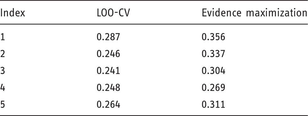
It seems that LOO-CV is strongly preferable when the training set is small. When data provided is insufficient, LOO-CV conditions more on the observation and hence uses less knowledge from the prior, which might be mis-specified. Notice that there is no guarantee that cross-validation is always better than evidence maximization in tuning the parameter: since cross-validation conditions too much on observations, there is a higher risk of over-fitting. Since GPR implemented here use both probabilistic loss function and evidence maximization as inference method, unsurprisingly it has relatively worse performance when the training set is a small one. On the other hand, there was no parameter initialization in GPR modeling (where in the LS-SVMs modeling CSA was employed to find suitable start values on hyper-parameters), which makes it more vulnerable to bad local minima for small training set cases. However, this could be an advantage when training set size is large, because it is more computationally efficient.

Conclusion

Three models, PLSR, LS-SVMs, and GPR, were introduced and studied on a large NIR spectroscopic data set. The averaged ratio of PLS/LS-SVMs and PLS/GPR on RMSEV were 1.270 and 1.300 correspondingly. The two non-linear models had similar performances and both improved significantly on PLSR. There was no strong evidence to indicate any significant differences in global bias between the three models. In PLSR, fitting power was not adequate to model the genuine non-linear relationship between NIR and target analyte, which led to a large bias and error when predicting samples with extremely high concentration. Non-linear models including LS-SVMs and GPR can effectively correct the non-linear deviation for extreme samples. Prediction accuracy for all of three models grows with an increasing training set. LS-SVM is strictly better than PLSR, independent of the size of calibration set. GPR has poor prediction performance when the training set is small, due to the characteristic of the evidence maximization process. However, the performance improves quickly when more samples are included in the calibration process, and soon becomes non-distinguishable from LS-SVMs.

Footnotes

Declaration of conflicting interests

The author(s) declared no potential conflicts of interest with respect to the research, authorship, and/or publication of this article.

Funding

The author(s) received no financial support for the research, authorship, and/or publication of this article.

References

Roggo

Chalus

Maurer

. A review of near infrared spectroscopy and chemometrics in pharmaceutical technologies. J Pharm Biomed Anal 2007; 44: 683–700.

Chen

Morris

Martin

. Gaussian process regression for multivariate spectroscopic calibration. Chemometrics Intell Lab Syst 2007; 87: 59–71.

Chen

Zhao

Fang

. Feasibility study on identification of green, black and oolong teas using near-infrared reflectance spectroscopy based on support vector machine (SVM). Spectrochim Acta A 2007; 66: 568–574.

Borin

Ferrao

Mello

. Least-squares support vector machines and near infrared spectroscopy for quantification of common adulterants in powdered milk. Anal Chim Acta 2006; 579: 25–32.

Widjaja

Zheng

Huang

. Classification of colonic tissues using near-infrared Raman spectroscopy and support vector machines. Int J Oncol 2008; 32: 653–662.

Zhang

Cong

Xie

. Quantitative analysis of routine chemical constituents in tobacco by near-infrared spectroscopy and support vector machine. Spectrochim Acta A 2008; 71: 1408–1413.

Gibson

Aigrain

Roberts

. A Gaussian process framework for modeling instrumental systematics: application to transmission spectroscopy. Monthly Notices R Astron Soc 2012; 419: 2683–2694.

Verrelst

Alonso

Caicedo

JPR

. Gaussian process retrieval of chlorophyll content from imaging spectroscopy data. IEEE J Select Top Appl Earth Observ Remote Sensing 2013; 6: 867–874.

Chen

Wang

. Bayesian variable selection for Gaussian process regression: application to chemometric calibration of spectrometers. Neurocomputing 2010; 73: 2718–2726.

10.

Thissen

Pepers

Üstün

. Comparing support vector machines to PLS for spectral regression applications. Chemometr Intell Lab Syst 2004; 73: 169–179.

11.

Wold S, Martens H and Wold H. The multivariate calibration problem in chemistry solved by PLS method. In: Proc. conf. matrix pencils (eds A Ruhe and B Kagstrom), Lecture notes in mathematics, piteå, Sweden, March 1982, Heidelberg: Springer-Verlag, pp.286–293.

12.

Martens H and Jensen SA. Partial least squares regression: a new two-stage NIR calibration method. In: Progress in cereal chemistry and technology, 1983, Amsterdam: Elsevier, Vol. 5a, pp.607–647.

13.

Martens H and Naes T. Multivariate calibration. New York: John Wiley & Sons, 1992.

14.

Suykens JA, Van Gestel T, De Brabanter J, et al. Least squares support vector machines. Vol. 4. Singapore: World Scientific, 2002.

15.

Kuhn HW and Tucker AW. Nonlinear programming. In: Proceedings of the second Berkeley symposium on mathematical statistics and probability, Berkeley, CA: University of California Press, August 1951, pp.481–492.

16.

Rasmussen CE. Gaussian process for machine learning. London: The MIT Press, 2006.

17.

Pelckmans K, Suykens JA, Van Gestel T, et al. Ls-svmlab: a matlab/c toolbox for least squares support vector machines. Tutorial. KULeuven-ESAT, Leuven, Belgium, 2002.

18.

Rasmussen

Nickisch

. Gaussian processes for machine learning (GPML) toolbox. J Machine Learn Res 2010; 11: 3011–3015.

19.

Xavier-de Souza

Suykens

Vandewalle

. Coupled simulated annealing. Syst Man Cybern B 2010; 40: 320–335.

20.

Fearn

. Comparing standard deviations. NIR News 1996; 7: 5–6.

21.

Fearn

Pérez-Marín

Garrido-Varo

. Inverse, classical, empirical and non-parametric calibrations in a Bayesian framework. J Near Infrared Spectrosc 2010; 18: 27.

22.

Wahba G. Spline models for observational data. Philadelphia: Siam, Vol. 59, 1990.