FII Profitability and Market Uncertainty: An Emerging Economy Context

Abstract

This study aims to uncover differences in profitability and market timing skills of Foreign Institutional Investors (FIIs) against benchmarks. Using a Markov Regime Switching Model, the article comments on the extent of information utilization by FIIs during periods of low and high economic uncertainty across global (NASDAQ-Composite 3000) and local markets (NIFTY-500 index). The results show significant over-performance (under-performance) in FIIs against benchmarks (NIFTY-50 and NIFTY-500 indices) during low (high) market uncertainty for local uncertainty. However, there is no significant difference in the overall profitability of FIIs during events of global economic uncertainty. The analysis utilizes precise estimates by taking all companies within the index individually and maintaining holdings for all. The article utilizes profitability measures of cash flows, Modified Internal Rate of Return and Buy-and-Hold-returns. The results of this study are relevant to institutional investors, policymakers and investors, especially during local and global uncertainty events.

Keywords

Accounting and finance business economics finance international relations

Introduction

The role and presence of Foreign Institutional Investors (FIIs) as active stakeholders in the Indian equity market have taken a position of incredible importance in recent times. India recorded its peak FII Inflow in the financial year 2021, a total of $37.6 billion, which is greater than the cumulative inflows over the last 6 years. This article attempts to answer the question of whether FIIs handle market uncertainty better than benchmarks. In other words, the study explores the ability of FIIs to handle information about volatility and comment on their profitability during times of global and local market uncertainty. Such information derives meaningful insight—if FIIs underperform against benchmarks in times of increased local uncertainty, it implies that FIIs are suffering from a local informational disadvantage on a corporation/market-specific level and is indicative of an increased level of information asymmetry within a particular market. Similarly, if FIIs overperform against benchmarks in times of increased global uncertainty, it indicates that FIIs have an information advantage with respect to global data.

To address this question, a Variance Regime Switching Markov Model is used to model market uncertainty for NIFTY-500 (local) and NASDAQ-Composite 3000 (global) indices. Within the achieved low and high-variance regimes for each, the Modified Internal Rate of Return (MIRR) is employed to define our profitability during the horizon. The results reflect that first, FIIs statistically underperform the benchmark (NIFTY-50 index) during periods of high local uncertainty and volatility. However, there is a statistically and practically significant edge that FIIs have over benchmarks during local low-variance regimes. It indicates that FIIs may indeed have the ability to leverage global information (in terms of exports, commodity prices, derivative markets and foreign exchange rates amongst others) to drive local returns while also being handicapped in their handling and leveraging of local information to perform at par with benchmarks during higher overall volatility. The results remain robust to using the NIFTY-500 index as the benchmark. Second, for uncertainty events within NASDAQ-Composite (global uncertainty), that there is no statistically significant difference between the performance of FIIs and benchmarks during events pertaining to global market uncertainty. This shows that FIIs that choose to invest in India, on average, do not enjoy an information advantage in the context of global variables and exposure to the same.

Although a few articles study FII transactions, the current study adds to the literature in many ways. First, the period of our study is bifurcated into bull and bear regimes, to identify the presence of a cyclical effect in over and underperformance of FIIs against benchmarks. This is perhaps the first article to incorporate varying market conditions. Second, unlike previous articles that use the net cash flow normalized for NIFTY-50 closing price, assuming that the entire cash flow goes into buying index units; the study takes all the 500 companies within the NIFTY-500 index individually and maintain holdings for all. This gives more precise estimates. Our results remain robust to using NIFTY-50 or NIFTY-500 indices as benchmarks for uncertainty. Third, although many articles study the difference in FII flows during major events, this article moves one step ahead and analyses profitability using cash flows and MIRR. The results of this study are relevant to institutional investors who may want to analyse the information scenario and allocate funds to passive or active fund managers. The findings of our study are also relevant to policymakers as the information environment affects the flow of funds and overall investment into the country’s assets. The market perceives that FIIs have the power to move the market. Assuming the perception to be true, this power can be used by them to do transactions to their benefit and at the cost of other investors. Thus, studying the profitability of FIIs has important policy implications. Analysing FIIs is also critical for retail investors. By learning about FII profitability, investors can identify potential investment opportunities and make informed investment decisions. Investors can identify opportunities to invest in different asset classes and sectors. Lastly, FII investments are often influenced by global economic trends and geopolitical events. By learning about FII profitability, investors can stay informed about global economic trends and events that may impact their FII investments. The results become more relevant as COVID-19 unfolds and this causes changes in the fund flow.

The flow of the article is as follows. The next section section reviews the relevant literature, while the subsequent two sections outline the data and methodology used, respectively. Results are discussed in the penultimate section. The last section concludes.

Literature Review

Many studies in different emerging markets analyse and discuss the strategies of FIIs and their overall profitability over different horizons. These studies have resulted in a mixed set of conclusions as these studies majorly consider two kinds of hypotheses—FII underperformance and FII overperformance.

According to several studies, FIIs’ ability to turn a profit is limited by their lack of access to information about the companies they might choose to invest in. By examining the impact of knowledge asymmetry on the company supporting the invested security, these studies evaluate this notion. According to Coval and Moskowitz (1999), geographic proximity has a significant impact on the choice of securities for domestic portfolios. In their analysis of the Jakarta stock exchange, Dvorak (2005) identified empirical evidence that foreign investors perform worse than domestic investors. However, Agarwal et al. (2009) found that overseas investors perform worse than their local counterparts when non-initiated buy-and-sell orders are taken into account. They also discovered that there was no substantial difference in performance in a causal relationship with proximity to financial centres or the corporate headquarters of the traded firm, which is evidence against information advantage. All of these instances show that FIIs underperform in comparison to domestic institutional investors (DIIs) and benchmarks, with the effect being stronger in businesses with larger levels of information asymmetry. The ideas that explain how DIIs have an advantage over FIIs in terms of the operational environment of the firms owing to the difference in geographic closeness support the hypotheses. Controlling for business variables, Bae et al. (2008) looked at the performance gaps between domestic and international analysts within a sample of 32 nations and found that these gaps were statistically and economically significant in favour of analysts living close to one another. When Hau (2001) examined international investors in the German equity market across eight European nations, she discovered that those who were based in non-German-speaking cities underperformed significantly.

Despite the wide set of reasons that give DIIs a considerable information edge in terms of qualitative and quantitative proximity, FIIs may have an information advantage in consideration of their access to global expertise, their exposure to global uncertainty and their handling of the same. FIIs have access to a much greater volume of information regarding the performance of assets in their portfolio diversified within a large array of different markets. Managers of such funds may have increased access to talent and may be able to handle global variables and their effect better within individual markets, thus complementing their information advantage. Oh et al. (2008) found foreign institutions to be the most profitable investors after local institutions and individual investors in the Korean market while Bae et al. (2011) found that foreign investors can distinguish superior opportunities in the Korean equity market in the short term. Similarly, Kim and Yi (2015) in their study of the Korean market, a market that has a high amount of exposure to global variables due to their dependence on foreign trade, found that despite the geographical and cultural constraints, FIIs have a relative information advantage. On the contrary, Choe et al. (2004) in their study of the Korean market, found that foreign investors underperform due to poor market timing skills in comparison to their domestic competitors.

Grinblatt et al. (2000) found in their study of the Finnish stock market an underlying level of sophistication and superior performance expressed through the trading strategies employed by FIIs against domestic institutions and individuals. Even after controlling for contrarian and momentum effects, they found significantly superior performance amongst FIIs. Similarly, Seasholes (2000) studied the same within the Taiwanese market and put forward the argument that access to better expertise provides for superior performance through empirical evidence that net foreign purchasing (selling) precedes positive (negative) earnings surprises. Bae et al. (2006) and Kamesaka et al. (2003) found that foreign investors come out on top in consideration of the Tokyo Stock Exchange due to their superior strategies and market timing skills. Shukla et al. (1995) found that UK funds underperform on their US investments in comparison to funds native to the United States. Froot and Ramadorai (2001) provided further evidence of the same through a cross-sectional study of 25 countries where they find that cross-border institutional investments are likely to be predictive of future returns locally. Iwatsubo et al. (2021), in a more recent context, found that due to the increasing importance put on globally available information over the recent decades, foreign investors trade at an information advantage.

In the context of the Indian market, Jain et al. (2016) showed that fund flows from FIIs (DIIs) significantly (do not) affect stock market returns. Using vector autoregression (VAR) methods, the article shows that FIIs buy more stocks when markets rise and sell more when markets are down. Arora (2016) provided evidence of a negative relation between FII investment and stock returns. Srinivas et al. (2015) demonstrated that Indian and United States equity markets affect FII inflows. Choudhary et al. (2022) exhibited a significant relationship between the herding behaviour of FIIs and stock market returns. Chauhan et al. (2020) found that FIIs engage in positive feedback trading whereas DII follow value investments in the Indian stock market. Badhani et al. (2020) found that foreign portfolios underperform domestic benchmark portfolios suggesting inferior market timing skills in the same market. Their methodology uses the net cash flow and divides it by the NIFTY-50 closing price to get daily holdings and assumes the entire cash flow goes into buying index units of the NIFTY-50. However, this study takes transactions specific to 500 companies and individually maintain holdings for all.

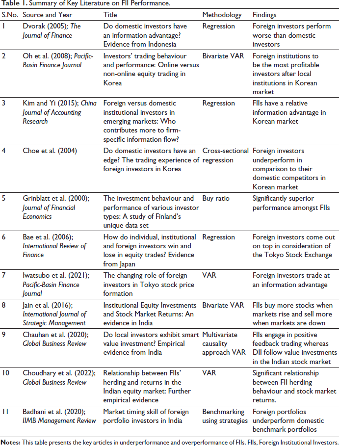
Considering the literature as it stands, studies have been conducted extensively to find the presence of over- or under-performance in FIIs in the context of local institutions and benchmarks (summarized in Table 1). These studies have the phenomenon of information asymmetry as a principal driver of performance variation. However, the study fills many research gaps in the literature. First, the variation in performance during varying conditions in the market is a phenomenon less studied. The period of our study is bifurcated into bull and bear regimes, to identify the presence of a cyclical effect in over and underperformance of FIIs against benchmarks. This is perhaps the first study that takes a cyclical approach to identify performance variation. Second, prior articles that use the net cash flow normalized for NIFTY-50 (benchmark) closing price assume that the entire cash flow goes into buying index units. The current study addresses the assumption and takes all the 500 companies within the NIFTY-500 index individually and maintain holdings for all. This gives more precise estimates. Third, although many articles study the difference in FII flows during major events, the article moves one step ahead and analyses profitability using cash flows and MIRR. Cash flows capture true value as opposed to accounting value, whereas MIRR encompasses time value of money effects. Hence, FII profitability is analysed against global and local uncertainty, in low and high variance regimes, making it one of the most comprehensive studies on FII performance.

Table 1.

Summary of Key Literature on FII Performanc

S.No.	Source and Year	Title	Methodology	Findings
1	Dvorak (2005) ; The Journal of Finance	Do domestic investors have an information advantage? Evidence from Indonesia	Regression	Foreign investors perform worse than domestic investors
2	Oh et al. (2008); Pacific-Basin Finance Journal	Investors’ trading behaviour and performance: Online versus non-online equity trading in Korea	Bivariate VAR	Foreign institutions to be the most profitable investors after local institutions in Korean market
3	Kim and Yi (2015); China Journal of Accounting Research	Foreign versus domestic institutional investors in emerging markets: Who contributes more to firm-specific information flow?	Regression	FIIs have a relative information advantage in Korean market
4	Choe et al. (2004)	Do domestic investors have an edge? The trading experience of foreign investors in Korea	Cross-sectional regression	Foreign investors underperform in comparison to their domestic competitors in Korean market
5	Grinblatt et al. (2000); Journal of Financial Economics	The investment behaviour and performance of various investor types: A study of Finland’s unique data set	Buy ratio	Significantly superior performance amongst FIIs
6	Bae et al. (2006); International Review of Finance	How do individual, institutional and foreign investors win and lose in equity trades? Evidence from Japan	Regression	Foreign investors come out on top in consideration of the Tokyo Stock Exchange
7	Iwatsubo et al. (2021); Pacific-Basin Finance Journal	The changing role of foreign investors in Tokyo stock price formation	VAR	Foreign investors trade at an information advantage
8	Jain et al. (2016); International Journal of Strategic Management	Institutional Equity Investments and Stock Market Returns: An evidence in India	Bivariate VAR	FIIs buy more stocks when markets rise and sell more when markets are down
9	Chauhan et al. (2020); Global Business Review	Do local investors exhibit smart value investment? Empirical evidence from India	Multivariate causality approach VAR	FIIs engage in positive feedback trading whereas DII follow value investments in the Indian stock market
10	Choudhary et al. (2022); Global Business Review	Relationship between FIIs’ herding and returns in the Indian equity market: Further empirical evidence	VAR	Significant relationship between FII herding behaviour and stock market returns.
11	Badhani et al. (2020); IIMB Management Review	Market timing skill of foreign portfolio investors in India	Benchmarking using strategies	Foreign portfolios underperform domestic benchmark portfolios

Notes: This table presents the key articles in underperformance and overperformance of FIIs. FIIs, Foreign Institutional Investors.

Methodology

Methodology Overview

Using the daily FII equity inflow and outflow data obtained from National Securities Depository Limited (NSDL) and closing prices from the CMIE ProwessIQ Database, the operational variable of Cash Flow and Holdings are generated which is the principal time series that the analysis is conducted over. Our measure of profitability is defined as the MIRR calculated on a range of cash flows that happen during a given time period. Once the cash flow time series and a measure of profitability are computed, a benchmark simulator, a Buy-and-Hold simulator, to measure FII performance against is identified and implemented.

In line with our intention to study the variance in over or underperformance during cyclical regimes in the market, a two-state switching Markov regression model is used to model the market into high and low-variance regimes. The stationarity of the NIFTY-500 series is verified using the Augmented Dickey-Fuller Unit Root test as is necessary for the extraction of the regimes.

Once the bull and bear regimes are generated, the MIRR of the FII cash flows and the benchmark during each regime are calculated. A dummy variable for whether the regime is a bull or bear regime is also defined. Subsequently, an ordinary least squares regression is run to regress the spread in the performance variables against the dummy variable to drive results.

Data

The daily FII inflow and outflow data for the equity time series have been obtained from NSDL. Under the 2014 SEBI Regulations, Foreign Portfolio Investors (FPI) as a term encompass institutional investors, sub-accounts and smaller accounts that were permitted to invest overseas, called qualified foreign investors. FPIs and FIIs are used interchangeably in literature and within our study as well. The data consists of trade-wise FII equity trade reports that record traded price, volume and nature of individual security transactions in the secondary market. The sample period spans from 31 December 2002 to 10 October 2020 (data availability at the time of commencement of the study). A large sample period captures the effects of high volatility events like the 2007 financial crisis as well as the recent COVID-19 pandemic. Only securities that are constituents of the Nifty-500 index (96.1% of the free-float market capitalization of all listed NSE stocks; Jain et al. (2019)) are considered. The closing prices for individual securities are obtained from the CMIE ProwessIQ Database. The NIFTY-50 and NIFTY-500 index values are obtained from NSE. Closing prices are converted into continuously compounded log returns for analysis.

Tools

Profitability Metrics

To analyse the profitability and market timing skills of FIIs against benchmark portfolios using passive investment strategies, the MIRR is used as the principal measure of profitability during a horizon. This measure is used across both FII Flows and passive Buy-and-Hold strategies.

The MIRR is calculated as follows. Given a certain set of cash flows, we treat the cash flows as a solitary investment with a subsequent booking of profits at the end of the horizon under consideration. Investments or buying of securities are treated as a negative cash flow while the action of squaring off and profit booking is treated as positive cash flow (booked profit). All the positive cash flows are compounded to the final day of the horizon, that is, Day N. Symmetrically, all the negative cash flows (investments) are discounted to Day 0, that is, the beginning of the horizon. The discount and compounding rate used is 8% annually (Badhani & Kumar, 2020). These are modelled as:

{PV}_{0} = \sum_{t = 0}^{t = n} {CF}_{t} * e^{- r t} for CF < 0

{FV}_{n} = \sum_{t = 0}^{t = n} {CF}_{t} * e^{r (n - t)} for CF > 0

M I R R = L n (1 + R) = \frac{L n ({FV}_{n}) - L n ({PV}_{0})}{n}

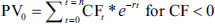
where PV denotes present value, FV denotes future value, r is the discounting/compounding rate, CFs denotes cash flows and n is the total number of days in the horizon.

Variance Regime Switching Model

This section analyses the ability of FIIs to maintain profitability during periods of high market uncertainty using previously constructed measures of profitability across FIIs and benchmarks. To model market uncertainty and extract high and low variance regimes, a 2-State Markov Variance Regime Switching model (MS-AR (2)) on NIFTY-500 is used. The stability of this model is also demonstrated by the high self-transition probabilities derived by the regression indicating two existing and stable regimes.

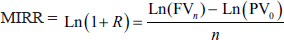
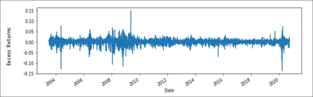
The analysis assumes that markets are divided into traditional cyclical regimes such as the bull-bear regime, justifying a two-state model (Mishra et al., 2020). The model tries to emulate a bull regime in the form of a low-variance stable regime with higher overall returns and a bear regime as a regime with a relatively higher level of uncertainty and lower returns. The NIFTY-500 stock returns are modelled as continuously compounded log returns. The stationarity of the time series is verified using the Augmented Dickey-Fuller Unit Root Test (Table 2). Stationarity is a necessary condition for the time series to be fed into a Markov Regressor. The time series is modelled using a Markov Regressor with variances switching over two regimes. Figure 1 plots the time series for the NIFTY-500 index for the entire sample period. It can be seen that the returns are heteroscedastic and variable variances justify modelling the series with a switching model. Figure 2 presents the smoothed probabilities of individual local variance regimes over the period of consideration..

Table 2.

Examining Stationarity on NIFTY 500 Time Series.

Time Series: NIFTY 500 Log Returns
Test-statistic	–13.91779
p Value	5.364e–26

Notes: This table presents the results of the Augmented Dickey-Fuller Unit Root Test on the time series of NIFTY-500 log returns over the sample period.

Figure 1.

Daily Continuously Compounded Log Excess Returns for NIFTY-500 Index over the Period 2003 to 2020. The Returns are Heteroscedastic Across the Sample Period.

Figure 2.

Smoothed Probabilities of Individual Local Variance Regimes.

Variables

FII Portfolio Simulator

Closely following Badhani and Kumar (2020), cash flows (CFs) are calculated using the daily flow data, and the subsequent value of holdings is recorded to find the initial and terminal value of the portfolio. The former is formally defined as

{Cash Flow}_{i} = \sum_{t = 1}^{t = (n - 1)} {CF}_{i, t}

(1)

where CF_i,t is the signed transaction value in INR of the trade t on Day i.

While recording the initial and terminal value of holdings, a long-only rule is followed, that is, companies are only allowed to sell securities that they previously own. This is done to ensure that at no point in time in the entire horizon, the value of the holdings goes to zero. Hence, the holdings are offset such that the absolute minimum value of holdings remains greater than or equal to zero. The total amount in holdings held across each company is

N_{t} = N_{0} + \sum_{i = 1}^{t} U_{t}

(2)

and,

N_{0 =} | \min (M) | if M < 0

N_{0} = 0 if M > 0

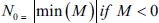
where N_t is the number of units held at time t, N₀ is the number of units held initially and U_t is the signed number of units held before the offset, obtained by the summation of all transactions occurring at time at any time t. M is defined as the minimum value of the raw holdings before the offset at time t.

To calculate the value of the initial and terminal number of units held for each company, the company-wise holdings data are utilized as follows:

[{Holdings Value}_{i, t}] = [{Holdings}_{i, t}] * [{Closing Price}_{i, t}]

(3)

Here i represents the security and t, is the day under consideration. If the terminal cash flows on Day 0 and Day n are required, the closing prices of each individual security are multiplied with its holdings and that becomes the net terminal cashflow for that day.

Benchmark Simulator

To quantify the relative performance of FIIs, a passive investment strategy is simulated using a Buy-and-Hold strategy (Badhani & Kumar, 2020). The simulated strategy assumes the investment (or negative flow) of one Rupee on Day 0 of the investment horizon, and the terminal cash flow is the price of the net holdings.

The amount in holdings on Day 0 is calculated using the closing price on the same day:

{Holdings}_{0} = \frac{1}{Index Close on Day 0}

(4)

The final cash flow is calculated:

{Cash Flow}_{n} = ({Holdings}_{0}) * (Index Close Day N)

(5)

The MIRR of such a portfolio is then computed as:

M I R R = \frac{L n (Index Close on Day N)}{No. of Days}

(6)

Performance Spread and Indicator Variable

To analyse the difference in profitability, the variable spread is defined as the difference between FII profitability and benchmark returns for the same period of time. This serves as the regression sample with Performance Spread (FII returns minus benchmark returns) as the dependent variable and Indicator as a dummy variable that takes a value of 1 for low-variance regimes and 0 for high-variance regimes.

Results

Summary Statistics

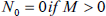
Panel A of Table 3 presents the summary statistics of the cash flow data set extracted from the sum value of transactions each day as well as of all transactions taken individually across all days within the horizon. It can be observed that on average, there are half a billion (INR) in cash inflows from FIIs. The skewness and median values of the cash flow data indicate a positively skewed distribution. Panel B presents the summary statistics of the NIFTY-50 closing price dataset used to model the benchmark simulators that are used to define the absolute spread. Panel C presents the summary statistics of the final regression sample used to drive inferences in Section 5.4.1.

Table 3.

Summary Statistics of FII Cash Flows and Benchmarks.

Panel A: Descriptive Statistics for FII Cash Flows and Transaction Values in INR
	Daily Net Cash Flows	Value of Each Transaction in INR	Transaction Rate	Transaction Volume
Minimum	–6.4E + 10	0	0	1
Maximum	1.76E + 11	4.65E + 10	81,193.06	1.65E + 08
Median	0	3,574,986	462.9288	7,738
Mean	5.19E + 08	19,298,812	1,040.614	53,910.88
Variance	4.86E + 19	6.48E + 15	7,165410	1.16E + 11
Skewness	5.338178	103.4072	13.04625	138.161
Panel B: NIFTY-50 Benchmark Closing Prices over the Entire Horizon
NIFTY-50 Closing Prices
Count 4,437	Mean 6,045.996	Standard deviation 3,112.511	Minimum 9,24.3	Maximum 12,362.3
Panel C: Descriptive Statistics for the Final Regression Samples
	Indicator	FII Returns	Benchmark Returns	Absolute Spread
Count	66	66	66	66
Mean	0.5	0.42	0.369525	0.053443
Standard deviation	0.503831	1.846477	1.554957	1.008205
Minimum	0	–4.11767	–2.53111	–3.46431
Maximum	1	8.837242	5.632162	4.41268

Notes: Panel A presents the summary statistics of the cash flow data set extracted from the sum value of transactions each day while also presenting the statistics of all transactions taken individually across all days within the horizon. Panel B presents the summary statistics of the NIFTY-50 Closing Price dataset used to model the benchmark simulators that are used to define the absolute spread. Panel C presents the summary statistics of the final regression sample used to drive inferences in Section 5.4.1. FII, Foreign Institutional Investor.

Results on FII and Benchmark Profitability

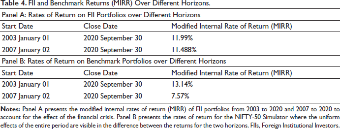
Panel A of Table 4 presents a comparison of the MIRR offered by a portfolio imitating the trading strategies employed by FII over the entire sample period and the MIRR accumulated annually from 2007 to the end of the sample period (financial crisis effect). It is observed that there is not much difference in the performance quantitatively, with a slightly higher rate during the full sample period. This may be because of the concentration of FII activity in the later periods of the horizon. This is one of the differentiating factors during the comparative study of FII performance against the study of benchmarks in the following section. Panel B presents the MIRRs of the benchmark index over the two time periods. Here a stark difference quantitatively can be seen between the two periods. It could be because there is a uniform depth of activity in terms of the benchmark portfolios in comparison to FIIs that are skewed towards periods much after the financial crisis. However, averaging over the entire horizon, benchmarks do slightly better than FIIs as their rate of return presents as 13.14% over the 12% offered by an FII portfolio.

Table 4.

FII and Benchmark Returns (MIRR) Over Different Horizons.

Panel A: Rates of Return on FII Portfolios over Different Horizons
Start Date	Close Date	Modified Internal Rate of Return (MIRR)
2003 January 01	2020 September 30	11.99%
2007 January 02	2020 September 30	11.488%
Panel B: Rates of Return on Benchmark Portfolios over Different Horizons
Start Date	Close Date	Modified Internal Rate of Return (MIRR)
2003 January 01	2020 September 30	13.14%
2007 January 02	2020 September 30	7.57%

Notes: Panel A presents the modified internal rates of return (MIRR) of FII portfolios from 2003 to 2020 and 2007 to 2020 to account for the effect of the financial crisis. Panel B presents the rates of return for the NIFTY-50 Simulator where the uniform effects of the entire period are visible in the difference between the returns for the two horizons. FIIs, Foreign Institutional Investors.

Variance Regime Switching Model

The results of the Variance Regime Switching Model regression are presented in Panel A of Table 5. We can assign low-variance states to traditional bull runs and high-variance states to bear runs due to the increased underlying market uncertainty. The variance parameter for the low variance regime is 7.689 × 10^–5 whereas the same parameter for the high variance regime is 6 × 10^–4. Both regression parameters are highly statistically significant. Panel B presents the transition probability matrix for the Markov Switching Process. The probability of the process staying in its previous state is high, indicating that the regression yields stable results.

Table 5.

Markov Variance Regime Switching Model Regression Summary Statistics.

Panel A: Regime Variance Parameters
Coefficient	Standard Error		p > \|Z\|		Z
Low-Variance Regime Parameters
Variance	7.689×10^-5		.000		24.313
High-Variance Regime Parameters
Variance	6 × 10^–4		.000		15.818
Panel B: Regime Transition Parameters
Transition States	Transition Probability	Standard Error	Z	p > \|Z\|	[0.025	0.975]
p[0 → 0]	.9885	0.003	392.941	.000	0.984	0.993
p[1 → 0]	.0368	0.008	4.704	.000	0.021	0.052

Notes: Panel A presents the results of the Markov Regression and presents the variance and stability parameters of State 0 (Low Variance) and State 1 (High Variance). Panel B presents the regime transition probabilities from to regime to another and from one regime to itself.

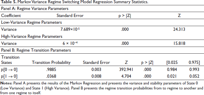
Figure 2 showcases the smoothed probabilities of the process being in a particular regime as a function of time. This helps us define bull and bear regimes over which to apply our profitability metrics and define the benchmark returns for the same. The expected duration of each regime in the process extracted from the regression parameters is 87 days for the low variance regime and about 27 days for the high variance alternative.

Effect of Local Variance Regimes on FII Profitability

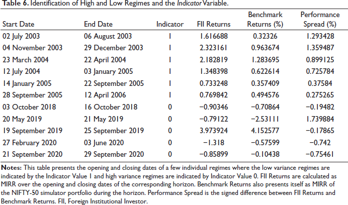
Once the various regimes are derived from the Markov Regression, the next step analyses the MIRR of the FII cashflows during that time and compares it using the Performance Spread variable. The regimes are indicated using the dummy variable Indicator. Here the low variance regimes are indicated by the Indicator Value 1 and high variance regimes are indicated by Indicator Value 0. To drive inferences, the model which regresses the Performance Spread against Indicator is run. Table 6 presents a subset of all the extracted regimes.

Table 6.

Identification of High and Low Regimes and the Indicator Variable.

Start Date	End Date	Indicator	FII Returns	Benchmark Returns (%)	Performance Spread (%)
02 July 2003	06 August 2003	1	1.616688	0.32326	1.293428
04 November 2003	29 December 2003	1	2.323161	0.963674	1.359487
23 March 2004	22 April 2004	1	2.182819	1.283695	0.899125
12 July 2004	03 January 2005	1	1.348398	0.622614	0.725784
14 January 2005	22 September 2005	1	0.733248	0.357409	0.37584
28 September 2005	12 April 2006	1	0.769842	0.494576	0.275265
03 October 2018	16 October 2018	0	–0.90346	–0.70864	–0.19482
20 May 2019	21 May 2019	0	–0.79122	–2.53111	1.739884
19 September 2019	25 September 2019	0	3.973924	4.152577	–0.17865
27 February 2020	03 June 2020	0	–1.318	–0.57599	–0.742
21 September 2020	29 September 2020	0	–0.85899	–0.10438	–0.75461

Notes: This table presents the opening and closing dates of a few individual regimes where the low variance regimes are indicated by the Indicator Value 1 and high variance regimes are indicated by Indicator Value 0. FII Returns are calculated as MIRR over the opening and closing dates of the corresponding horizon. Benchmark Returns also presents itself as MIRR of the NIFTY-50 simulator portfolio during the horizon. Performance Spread is the signed difference between FII Returns and Benchmark Returns. FII, Foreign Institutional Investor.

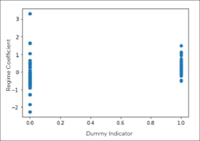
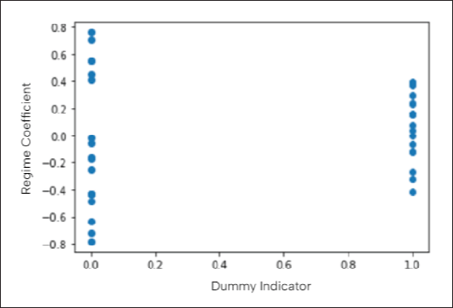
The scatter plot between Indicator and Performance Spread is shown in Figure 3. FII Spread is higher and more stable during low-variance bull regimes and FII returns tend to be lower and unstable during high-variance regimes.

Figure 3.

Scatter Plot of Local Performance Spread Against Dummy Indicator Regressor.

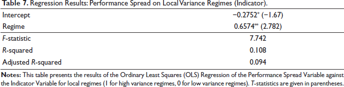
The above observation is corroborated statistically using a regression model. Table 7 shows that first, the value of the coefficient of the regime indicator is positive and significant at 1%, that is, during low variance regimes, the FII spread over the benchmark is positive and significant. This indicates that during regimes of low local uncertainty, FIIs are better at handling locally available information, have superior market timing skills, and have an overall higher degree of profitability. The underlying reasons that may allow FIIs to outperform benchmarks may involve access to a higher standard of talent and resources that are capable of establishing a higher degree of synergy with local information during low uncertainty. It could also indicate that the ability of FIIs to use global data to derive value out of global markets may be more pronounced during low variance periods. Second, the intercept is negative and significant. During periods of local uncertainty or high-variance regimes in the local market, FIIs underperform benchmarks. This could be due to their inability to handle or lack of access to local market information, especially during periods of higher uncertainty, an effect that presents itself as overall underperformance.

Table 7.

Regression Results: Performance Spread on Local Variance Regimes (Indicator).

Intercept	−0.2752^* (−1.67)
Regime	0.6574^** (2.782)
F-statistic	7.742
R-squared	0.108
Adjusted R-squared	0.094

Notes: This table presents the results of the Ordinary Least Squares (OLS) Regression of the Performance Spread Variable against the Indicator Variable for local regimes (1 for high variance regimes, 0 for low variance regimes). T-statistics are given in parentheses.

Effect of Global Variance Regimes on FII Profitability

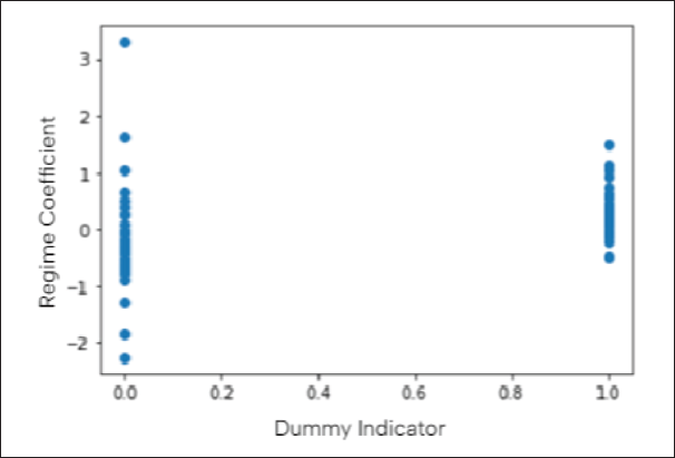
This section analyses FII performance for global uncertainty regimes as extracted from the NASDAQ-Composite 3000 index. The scatter plot for the dummy variable representing the profitability during particular regimes is presented in Figure 4. In comparison to Figure 3, it is observed that the dummy variables on regimes do not give a significant difference in the horizon profitability.

Figure 4.

Scatter Plot of Global Performance Spread Against Dummy Indicator Regressor.

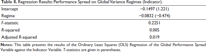
The inference from the figure is statistically corroborated in Table 8. There, the indicator regime variable is insignificant. Hence, there is no significant difference in the overall profitability of FIIs and benchmark during events of global economic uncertainty. FIIs do not seem to have any information advantage due to their access to global economic centres and the handling of global data is on par with or not significantly different from benchmarks.

Table 8.

Regression Results: Performance Spread on Global Variance Regimes (Indicator).

Intercept	−0.1497 (1.221)
Regime	−0.0832 (−0.474)
F-statistic	0.2251
R-squared	0.005
Adjusted R-squared	0.019

Notes: This table presents the results of the Ordinary Least Squares (OLS) Regression of the Global Performance Spread Variable against the Indicator Variable. T-statistics are given in parentheses.

Robustness Test with NIFTY-500 Benchmark

Previous sections analysed the performance of FIIs against NIFTY-50 benchmarks using individual fund flows for each company within the NIFTY-500. For robustness, the results from Effect of Local Variance Regimes on FII Profitability section are reproduced using NIFTY-500 for benchmarking.

Local Variance Regimes Against NIFTY-500 Benchmarks

This section analyses the performance of FII flows during low and high-variance periods derived from NIFTY-500 regimes and then compare their corresponding MIRR against that of the NIFTY-500 Buy-and-Hold Simulator. The scatter plot illustrating the effect of the dummy regime variable with regard to the NIFTY-500 FII Spread is presented in Figure 5.

Figure 5.

Scatter Plot of Local Performance Spread over NIFTY-500 Against Dummy Regressor.

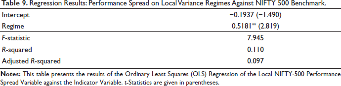
The figure shows that while the intercept variable is considerably dispersed, there is a statistically significant difference in the spread characteristics during low-variance regimes. The same theory is corroborated statistically by the regression values in Table 9. This shows that when a benchmark that follows the NIFTY-500 index is considered, FIIs have no edge during high-variance regimes, while they do considerably better during low-variance regimes, as earlier.

Table 9.

Regression Results: Performance Spread on Local Variance Regimes Against NIFTY 500 Benchmark.

Intercept	−0.1937 (−1.490)
Regime	0.5181** (2.819)
F-statistic	7.945
R-squared	0.110
Adjusted R-squared	0.097

Notes: This table presents the results of the Ordinary Least Squares (OLS) Regression of the Local NIFTY-500 Performance Spread Variable against the Indicator Variable. t-Statistics are given in parentheses.

Global Regimes Against NIFTY-500 Benchmarks

This section analyses the performance of FII flows during low and high-variance periods derived from NASDAQ-Composite regimes and then compare their corresponding MIRR against that of the NIFTY-500 Buy-and-Hold Simulator. Figure 6 illustrates the scatter plot of the effect of the dummy regime variable with regard to the NIFTY -500 FII Spread.

The results (Table 10) remain similar to the previous section. The intercept remains insignificant, while the regime variable is statistically significant and indicates an FII advantage during low variance regimes exclusively.

Table 10.

Regression Results: Performance Spread on Global Variance Regimes Against NIFTY 500 Benchmark.

Intercept	−0.1041 (−1.327)
Regime	0.1990^** (1.818)
F-statistic	3.304
R-squared	0.086
Adjusted R-squared	0.097

Notes: This table presents the results of the Ordinary Least Squares (OLS) Regression of the Local NIFTY-500 Performance Spread Variable against the Indicator Variable. T-statistics are given in parentheses.

Conclusion

Our study covers the effect of global and local market uncertainty on the profitability and market timing skills of FIIs. This study is based on the identification of variance in cyclical performance against benchmarks and this may be due to reasons such as information asymmetry in the context of geographical proximity to the firms. A Variance Regime Switching Markov Model is used to model market uncertainty for NIFTY-500 (local uncertainty) and NASDAQ-Composite 3000 (global uncertainty) indices. Within the achieved low and high variance regimes, the MIRR are used to define profitability during said horizon.

The results show that the FII spread over the benchmark (NIFTY-50, or NIFTY-500) is positive and significant during local low-variance regimes. This indicates that during regimes of low local uncertainty, FIIs are better at handling locally available information, have superior market timing skills, and have an overall higher degree of profitability. The underlying reasons may involve access to a higher standard of talent and resources that are capable of establishing a higher degree of synergy with local information during low uncertainty. During periods of high-variance regimes in the local market, FIIs underperform benchmarks. This could be due to their lack of access to local market information, especially during periods of higher uncertainty. We find that there are no significant differences in the spread between FII and benchmark performance during regimes extracted from NASDAQ-Composite 3000. FIIs do not seem to have any information advantage due to their access to global economic centres and the handling of global data is on par with or not significantly different from benchmarks.

Our article makes several implications. The study’s findings are pertinent to institutional investors who would want to evaluate the information circumstance and decide whether to fund active or passive fund managers. While the information environment influences the flow of money and overall investment into the nation’s assets, the results of our study are especially important for policymakers. The market believes that FIIs could influence market behaviour. If the perception is accurate, they may utilize this ability to carry out activities that would profit them at the expense of other investors. Therefore, researching FII profitability has significant policy ramifications. FII analysis is crucial for retail investors as well. Investors can find prospective investment opportunities and make wise investment selections by knowing about FII profitability. Investors can spot chances to invest in various asset classes and industries. Finally, geopolitical developments and global economic trends frequently have an impact on FII investments. Investors can stay informed about events and developments in the global economy that might affect their FII investments by studying FII profitability. As COVID-19 develops, the results become increasingly pertinent, changing the fund flow. As an extension the study, further research into the nature of the information environment of the underlying firms and the asymmetry in their access to the same may provide concrete determinants behind this spread in performance.

Footnotes

Acknowledgements

The authors are grateful to the journal’s anonymous referees for their extremely useful suggestions to improve the quality of the article. Usual disclaimers apply.

Declaration of Conflicting Interests

The authors declared no potential conflicts of interest with respect to the research, authorship and/or publication of this article.

Funding

The authors received no financial support for the research, authorship and/or publication of this article.

ORCID iD

Sonali Jain

References

Agarwal

, Faircloth

, Liu

, & Ghon Rhee

(2009). Why do foreign investors underperform domestic investors in trading activities? Evidence from Indonesia. Journal of Financial Markets , 12(1), 32–53. https://doi.org/10.1016/j.finmar.2008.04.001

Arora

R. K.

(2016). The relation between investment of domestic and foreign institutional investors and stock returns in India. Global Business Review , 17(3), 654–664. https://doi.org/10.1177/0972150916630830

Badhani

K. N.

, & Kumar

(2020). Market timing skill of foreign portfolio investors in India. IIMB Management Review , 32(1), 24–38. https://doi.org/10.1016/j.iimb.2019.07.012

Bae

K.-H.

, Stulz

R. M.

, & Tan

(2008). Do local analysts know more? A cross-country study of the performance of local analysts and foreign analysts. Journal of Financial Economics , 88(3), 581–606. https://doi.org/10.1016/j.jfineco.2007.02.004

Bae

K.-H.

, Yamada

, & Ito

(2006). How do individual, institutional, and foreign investors win and lose in equity trades? Evidence from Japan. International Review of Finance , 6(3–4),129–155. https://doi.org/10.2139/ssrn.500242

Bae

S. C.

, Min

J. H.

, & Jung

(2011). Trading behavior, performance, and stock preference of foreigners, local institutions, and individual investors: Evidence from the Korean stock market. Asia-Pacific Journal of Financial Studies , 40(2), 199–239. https://doi.org/10.1111/j.2041–6156.2011.01037.x

Chauhan

A. K.

, & Chaklader

(2020). Do local investors exhibit smart value investment? Empirical evidence from India. Global Business Review . https://doi.org/10.1177/0972150920915330

Choe

, Kho

B.-C.

, & Stulz

(2004). Do domestic investors have an edge? The trading experience of foreign investors in Korea (NBER Working Paper No. w10502). Available at SSRN. https://doi.org/10.3386/w10502

Choudhary

, Singh

, & Soni

(2022). Relationship between FIIs’ herding and returns in the indian equity market: Further empirical evidence. Global Business Review , 23(1), 137–155. https://doi.org/10.1177/0972150919845223

10.

Coval

J. D.

, & Moskowitz

T. J.

(1999). Home bias at home: Local equity preference in domestic portfolios. The Journal of Finance , 54(6), 2045–2073. http://www.jstor.org/stable/797987

11.

Dvořák

(2005). Do domestic investors have an information advantage? Evidence from Indonesia. The Journal of Finance , 60(2), 817–839. https://doi.org/10.1111/j.1540–6261.2005.00747.x

12.

Froot

, & Ramadorai

(2001). The information content of international portfolio flows (NBER Working Paper No. w8472). Available at SSRN. https://doi.org/10.3386/w8472

13.

Grinblatt

, & Keloharju

(2000). The investment behavior and performance of various investor types: A study of Finland’s unique data set. Journal of Financial Economics , 55(1), 43–67. https://doi.org/10.1016/S0304–405X(99)00044–6

14.

Hau

(2001). Location matters: An examination of trading profits. The Journal of Finance , 56(5), 1959–1983. https://doi.org/10.1111/0022–1082.00396

15.

Iwatsubo

, & Watkins

(2021). The changing role of foreign investors in Tokyo stock price formation. Pacific-Basin Finance Journal , 67, 101548. https://doi.org/10.1016/j.pacfin.2021.101548

16.

Jain

(2016). Institutional equity investments and stock market returns: An evidence in India. International Journal of Strategic Management , 16, 69–86. https://doi.org/10.18374/IJSM-16–1.6

17.

Jain

, Varma

J. R.

, & Agarwalla

S. K.

(2019). Indian equity options: Smile, risk premiums, and efficiency. Journal of Futures Markets , 39(2), 150–163. https://doi.org/10.1002/fut.21971

18.

Kamesaka

, Nofsinger

J. R.

, & Kawakita

(2003). Investment patterns and performance of investor groups in Japan. Pacific-Basin Finance Journal , 11(1), 1–22. https://doi.org/10.1016/S0927–538X(02)00095–1

19.

Kim

J.-B.

, & Yi

C. H.

(2015). Foreign versus domestic institutional investors in emerging markets: Who contributes more to firm-specific information flow? China Journal of Accounting Research , 8(1), 1–23. https://doi.org/10.1016/j.cjar.2015.01.001

20.

Mishra

A. K.

, Rath

B. N.

, & Dash

A. K.

(2020). Does the Indian Financial Market Nosedive because of the COVID-19 outbreak, in comparison to after demonetisation and the GST? Emerging Markets Finance and Trade , 56(10), 2162–2180. https://doi.org/10.1080/1540496X.2020.1785425

21.

N. Y.

, Parwada

J. T.

, & Walter

T. S.

(2008). Investors’ trading behavior and performance: Online versus non-online equity trading in Korea. Pacific-Basin Finance Journal , 16(1–2), 26–43. https://doi.org/10.1016/j.pacfin.2007.04.009

22.

Seasholes

(2000). Smart foreign traders in emerging markets (Working paper). Harvard Business School.

23.

Shukla

R. K.

, & van Inwegen

G. B.

(1995). Do locals perform better than foreigners? An analysis of UK and US mutual fund managers. Journal of Economics and Business , 47(3), 241–254. https://doi.org/10.1016/0148–6195(95)00009-G

24.

Srinivasan

, & Kalaivani

(2015). Determinants of foreign institutional investment in India: An empirical analysis. Global Business Review , 16(3), 364–376. https://doi.org/10.1177/0972150915569925