Histomorphometric,CT Arthrographic,and Biomechanical Mapping of the Human Ankle

Abstract

Background:

The specific morphological and biomechanical characteristics of the osteochondral unit of the ankle joint are not yet fully understood. This anatomical study aimed to map regional thickness of the articular hyaline uncalcified cartilage and its adjacent layers of mineralized cartilage and subchondral bone as well as to measure the regional indentation stiffness of human ankle joint cartilage.

Materials and Methods:

A total of 20 pairs of human cadaver ankle joints (median age: 78 years) were evaluated by histomorphometry and multidetector row double-contrast CT arthrography for cartilage thickness in 17 distinct anatomical regions. In addition, regional distribution of the subchondral bone plate and of the mineralized cartilage was scrutinized histologically. Cartilage indentation stiffness was measured using an arthroscopic handheld device (Artscan200), especially validated for use in thin cartilage. The correlation between the thickness of different components of the osteochondral unit and the cartilage indentation stiffness was evaluated.

Results:

The thinnest uncalcified cartilage was measured at the anterior talar dome and the distal fibula. The thickest uncalcified cartilage was found in the mid and posterior talar dome, as well as in the tibial plafond. Mineralized cartilage and subchondral bone showed highest values at the anteromedial talar dome. Cartilage indentation stiffness showed a bicentric distribution pattern in 14/20 ankle pairs and was highest in regions with thin cartilage. Positive correlation between the thickness of the mineralized cartilage and the subchondral bone plate was found. No correlation between the thickness of the uncalcified and the mineralized cartilage could be identified.

Conclusion:

This anatomical study provides a comprehensive mapping of the osteochondral unit of the human ankle joint in elderly people. Articular hyaline uncalcified cartilage and the subchondral bone plate showed clear regional differences and were reciprocally distributed. Cartilage indentation stiffness was inversely correlated to cartilage thickness in elderly people.

Clinical Relevance:

Thorough understanding of the osteochondral unit of the ankle joint could be helpful for clinicians and researchers in the development of improved operative repair techniques for osteochondral defects in the ankle joint, for example, in constructing specific tissue-engineered osteochondral plugs.

Keywords

ankle joint regional thickness hyaline uncalcified cartilage mineralized cartilage subchondral bone double-contrast CT arthrography cartilage indentation stiffness

Posttraumatic osteochondral defects are a major concern in orthopedic surgery,⁴³ whereas primary ankle joint osteoarthritis is a relatively rare event.^5,7,34 Although promising results in operative restoration of isolated cartilage defects have been reported,^12,13,31,37 important limitations in the treatment of osteochondral lesions of the ankle joint persist.^28,42 Comprehensive knowledge of joint specific anatomical design seems to be 1 of the key points for better understanding the biological demands on osteochondral regeneration. In contrast to other joints of the human body (ie, knee and hip joint), few studies in the past have focused on the specific anatomy and biomechanics of the osteochondral unit in the human ankle joint.^3,9,17,23,38

Therefore, this study was performed to provide insights into the regional histological configuration of the subchondral bone plate, its layer of mineralized cartilage, and the articular hyaline uncalcified cartilage in all areas of the human ankle joint. These histomorphometrical data were compared to each other and to double-contrast CT arthrography measurements of cartilage thickness to test the following hypotheses:

Hypothesis 1: The thickness of the subchondral bone plate, its layer of mineralized cartilage, and the articular hyaline uncalcified cartilage vary according to the localization within the human ankle joint.

Hypothesis 2: The thickness of the articular hyaline uncalcified cartilage at the talar shoulders is higher than the one at the center of the talus.

Hypothesis 3: The cartilage stiffness in the human ankle joint varies according to the localization and is inversely correlated to cartilage thickness.

Moreover, talus graphical analysis was performed to search for distinctive distribution patterns of cartilage and subchondral bone along with correlation analysis of regional subchondral bone plate, mineralized and articular hyaline uncalcified cartilage thickness with regional cartilage indentation stiffness.

The authors aimed to present histological and biomechanical mapping of the ankle joint osteochondral unit to improve understanding of the prerequisites for better surgical repair and promote the development of modern strategies like prefabricated tissue-engineered osteochondral plugs, specially designed for use in ankle joint defects.

Materials and Methods

Specimens

In all, 20 pairs of human cadaver ankle joints were obtained from donors of an affiliated pathologic institute. All specimens were acquired in accordance with state and federal laws. Local ethics committee approval was provided. The medical histories were reviewed for reports of prior ankle trauma and the presence of systemic musculoskeletal or rheumatoid diseases (exclusion criteria). The upper ankle joint was explored by a standard anterior approach and dissected from all adjacent soft tissues, except for the collateral ligaments. After sawing the distal tibia and fibula just above the anterior syndesmosis, the ankle joint was resected with the entire talus. Each specimen was visually examined for cartilage surface lesions according to the Outerbridge criteria.²⁹ None of the cadavers had to be excluded from the study and a total of 11 male and 9 female donors were available for CIS and histological analysis. For CT arthrography, 9 males and 9 females were available. Median age was 78 years (range, 34 to 89). Median time from donor’s death to CIS measurement was 20 hours (range, 11 to 24).

Double-contrast CT Arthrography

The samples were wrapped in polythene film and Iopamiro 300 radiopaque dye (Bracco Suisse SA, Mendrisio, Switzerland) diluted 1-to-1 in normal saline was injected into the ankle joint through the film. Double-contrast multidetector row CT arthrography was then performed with an ultrathin multislice technique (Siemens SOMATOM Sensation 16 scanner, Siemens, Erlangen, Germany; 16 × 0.75 mm collimation and convolution kernel B60s). For measurement purposes, 17 distinctive anatomic regions (1-17) on the talar dome, the tibial plafond and the distal fibula were defined for data analysis following the grid scheme of Elias et al (Figure 1).¹⁰ Median CT arthrography cartilage thickness (CT) was measured at 3 adjacent points at each of the 17 anatomic regions in the reconstructed sagittal plane by using radiological software (OsiriX, DICOM Viewer, 3.7.1, Pixmeo, Geneva, Switzerland). Additional CT measurements were performed in the coronal plane for the middle portion of the talar dome (corresponding to regions 4, 5, and 6).

Figure 1.

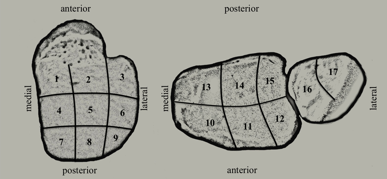
Grid scheme: On the left, view from above on the talar dome with regions 1 to 9; on the right, view from below on the tibial plafond with regions 10 to 15 and on the distal fibula with regions 16 and 17.

Cartilage Indentation Stiffness

Cartilage indentation stiffness measurement was performed using the Artscan200 arthroscopic handheld cartilage indentation stiffness tester (Artscan Oy, Helsinki, Finland) with the spherical-ended indenter (diameter 1 mm, height 0.3 mm) for thin cartilage. Five single measurements were repeated in the center of each of the 17 anatomic regions for calculation of the median cartilage indentation stiffness (CIS).

Histomorphometric Analysis

For histomorphometric analysis, the talus was separated from the tibio-fibular aspect of the ankle joint. Fixation and embedding of the samples in methylmethacrylate followed Erben’s protocol.¹¹ Anterior to posterior longitudinal sectioning in the sagittal plane was performed on the entire talus. Medial to lateral transverse sectioning in the coronal plane was performed on the distal tibia and fibula. Six slides with 10 µm thickness were obtained of each of the 17 anatomic regions. Trichrome Masson-Goldner (MG) staining was used for histology (Leica M205, Leica Microsystems, Nussloch, Germany). Digital photographs with different magnification were taken of each of the 17 anatomic regions for histomorphometric data analysis (Image Access Standard, Image Access, Wuppertal, Germany), according to the technique described by Pastoureau and Chomel for the tibial plateau.³⁰ Cartilage degeneration was documented histologically according to the OARSI grading system.³² For measurements of the histological thickness of the articular hyaline uncalcified cartilage (UC), of the mineralized cartilage (MC) and of the subchondral bone plate (SBP), digital photographs in 63-fold magnification were used and transferred to Image Access for further analysis. A 3000 μm line parallel to the tidemark was drawn in (defining the given length). The area above/below that line was traced for each of the anatomical structures (UC, MC, SBP). The sized area in μm² divided by the given length (3000 μm) provided the average height corresponding to the particular average thickness in the distinctive anatomic area.

Graphical Illustration and Statistical Analysis

Graphical illustration of regional UC and CIS distribution in color steps was carried out with Microsoft Office Excel (version 2003), following the technique of Milz.²⁴ Statistical analysis and the remaining graphical data display was performed by a statistician using Intercooled Stata Version 11.0 for Macintosh (StataCorp, College Station, Texas). Calculations of median CIS, UC, MC, SBP and CT, as well as of the interquartile ranges (IQRs) were performed on the particular average values of the 20 ankle pairs. These results were presented in box plots. The relationship of these different measurements was investigated by calculation of (nonparametric) Spearman’s rho correlation coefficients and presented in scatterplots with smoothed lowess curves. In consideration of the small sample size, we chose not to perform any significance tests to avoid type I errors. We decided to display the results graphically.

Definitions and Abbreviations

Table 1 gives an overview of the abbreviations used in this study.

Table 1.

List of the abbreviations frequently used in the text and figures.

UC	Thickness of the articular hyaline uncalcified cartilage measured by histology
MC	Thickness of the mineralized cartilage measured by histology
SBP	Thickness of the subchondral bone plate measured by histology
CT	Thickness of the articular cartilage measured by double-contrast CT arthrography
CIS	Cartilage indentation stiffness measured by the Artscan200 indenter

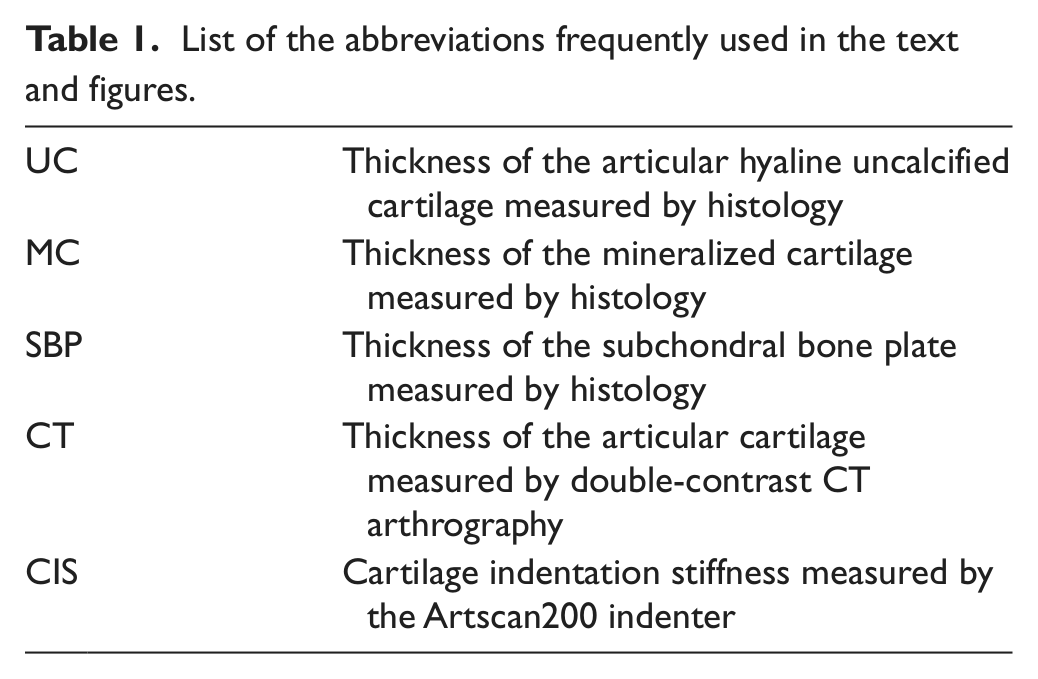
Duncan’s classification terminology for the SBP and the layers of mineralized and hyaline articular UC has been used in this study.⁸

Results

General Characteristics

In general, high symmetry was found between the left and right ankles regarding the single parameters UC, CT, SBP, MC, and CIS.

Cartilage Degeneration

Macroscopic and microscopic scoring of the articular cartilage in all 20 pairs of samples using the ICRS and OARSI grading system showed no or only minimal degenerative changes. Localized, more intense histological articular cartilage defects (OARSI > 1) appeared to be, in most cases, artifacts from the embedding and sectioning process and were not included in the histological measurements.

Histological Appearance of the Osteochondral Unit

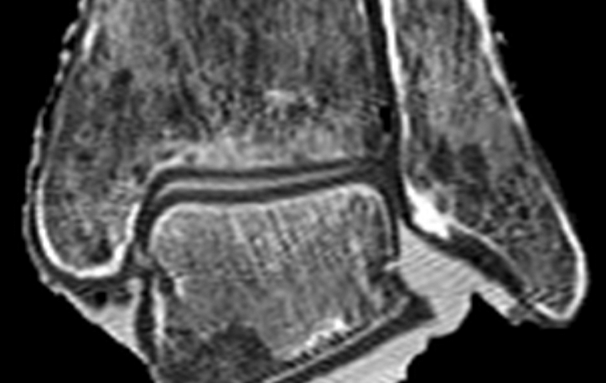
No cysts, microstructural fractures or inflammatory changes were found in the SBP or subarticular spongiosa of the talar dome, the tibial plafond and the distal fibula (Figure 2). The 3 layers (SBP, MC, articular hyaline UC) could be histologically well differentiated in all specimens. The zone of the articular hyaline UC showed the typical architecture of a superficial tangential layer, an adjacent transitional layer, and a radial layer at its base, followed by the layer of MC. These were separated by the wavy tidemark. The latter was easily distinguished in MG-staining by its pure purple-red dying. There were no replications of the tidemark noted in any of the specimens, indicating that no important osteoarthritic changes were present. Differentiation of the light green MC and the dark green lamellar subchondral bone was easily achieved in all of the specimens by identification of a jigsaw puzzle-like cement line.

Figure 2.

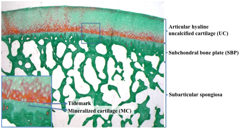
Example of a 25× magnification of a right mid talar dome, Trichrome Masson-Goldner staining. At the top, the layer of articular hyaline uncalcified cartilage (UC) with some orange-red dying of its radial layer, followed by the purple-red tidemark (see detail: short arrow). The SBP consists of the light green mineralized cartilage (MC; see detail: long arrow) and the dark green lamellar subchondral bone. Below, the subarticular spongiosa (cancellous bone, dark green).

Histological and CT Arthrography Cartilage Thickness

Overall, positive correlation (Spearman’s rho 0.61) was found between UC and CT for the talar dome and the tibial plafond, most distinctly in the range between 0.8 to 1.5 mm, where most of the data were located. Histological and CT arthrography median thickness of articular cartilage averaged over all 17 anatomic regions was 1.29 and 1.07 mm, respectively, and ranged from 0.96 to 1.68 mm and from 0.81 to 1.29 mm, respectively.

Talus

Graphical regional illustration of articular cartilage thickness distribution showed in 15 of 18 (CT) and in 17 of 20 (UC) ankle pairs a symmetrical monocentric pattern with highest UC and CT values posterior centrally and/or posterior medially (Figure 3). A bicentric pattern with UC peaks in regions 7 and 9 could only be clearly demonstrated in 2 ankle pairs. One ankle pair in each series (CT and UC) could not be strictly assigned to 1 of the 2 patterns. No ankle pair showed isolated peak cartilage thickness on the anterior aspect of the talar dome. Histological median UC and CT values in the 9 regions of the talar dome ranged from 1.08 to 1.50 mm and from 0.89 to 1.39 mm, respectively (Figure 4). UC was lowest in the anterior aspect (regions 1, 2, 3) and highest in the mid (regions 4, 5, 6) and posterior (regions 7, 8, 9) talar dome. In the mid talar dome, the highest UC values were found medially and centrally, whereas laterally, median UC was lower. Posteriorly, median UC was uniform within the 3 anatomic regions 7, 8, and 9. CT showed similar distribution patterns to UC, except for CT values consistently showing a decrease from the medial to the lateral talar dome in all anatomic regions. Moreover, CT ranged in all regions 0.1 to 0.35 mm below the UC values. In the posterior aspect of the talar dome, the differences were most distinct. In addition to the sagittal plane, talus cartilage was also evaluated in the coronal plane in regions 4, 5, and 6—the thickest cartilage was shown directly over the medial and lateral edges of the talar dome (Figure 5).

Figure 3.

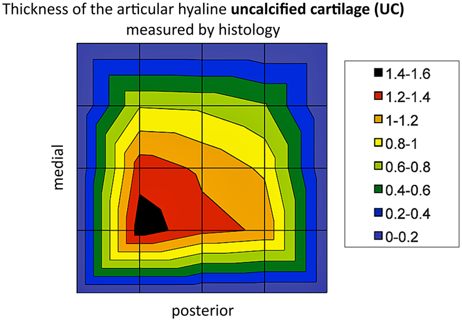
Example of a monocentric pattern of regional UC distribution in the talar dome represented in color steps of 0.2 mm, black 1.4 to 1.6 mm, dark green 0.4 to 0.6 mm.

Figure 4.

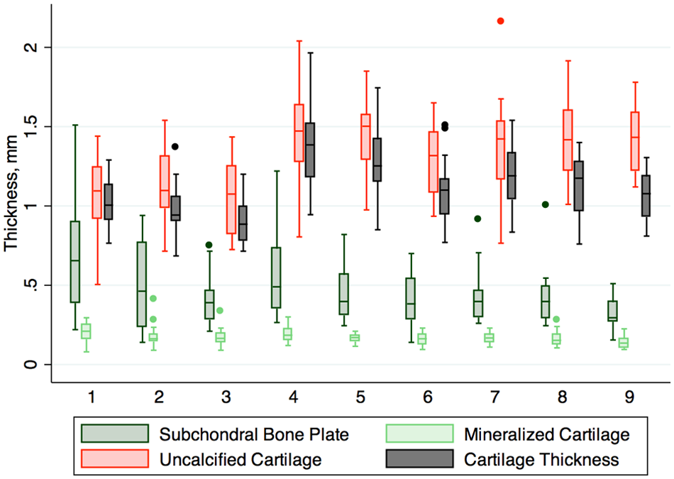
Box plot 1: Illustration of regional thickness distribution in mm of SBP (dark green), MC (light green), UC (red), and CT (black) in the box plot of the talar dome, regions 1 to 9, following the grid scheme.

Figure 5.

Double-contrast CT-Arthrography imaging of the mid talar dome (corresponding to regions 4, 5, 6) in a reformatted coronal plane. At the medial and lateral talar edges, cartilage thickness is higher than centrally.

Distal tibia and fibula

Histological median UC and CT values in the tibial plafond ranged from 1.24 to 1.46 mm and from 0.85 to 1.28 mm, respectively (Figure 6). CT was thickest close to the medial malleolus (regions 10 and 13) and showed a constant decrease toward the lateral aspect of the tibial plafond (regions 12 and 15). CT values in all regions ranged 0.08 to 0.39 mm below UC. At the fibular side, differences between CT and UC were likewise evident. CT values were 0.17 to 0.29 mm below UC. Median UC for the proximal fibular region was 0.87 mm, for the distal region 0.98 mm.

Figure 6.

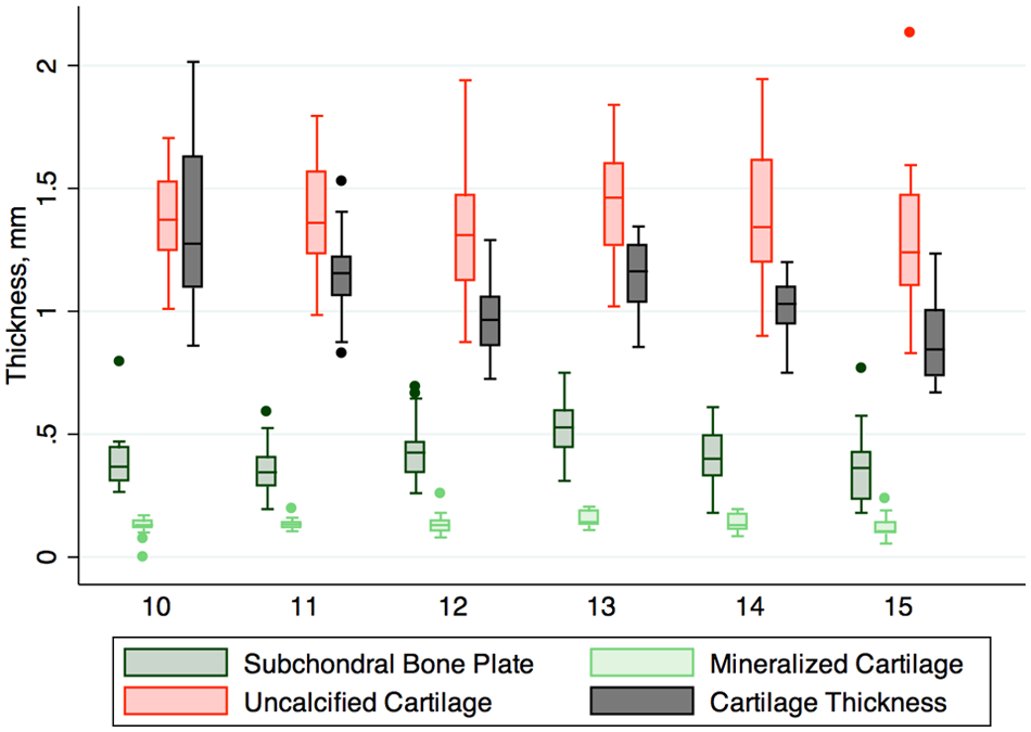
Box plot 2: Illustration of regional thickness distribution in mm of SBP (dark green), MC (light green), UC (red), and CT (black) in the box plot of the tibial plafond, regions 10 to 15, following the grid scheme.

Histological Evaluation of the Subchondral Bone Plate

Overall, positive correlation (Spearman’s rho 0.47) was found between SBP and MC for the talar dome, the tibial plafond and the distal fibula, most distinct in the range between 0.2 to 0.6 mm, where most of the data were located (Figure 7). No obvious correlation could be found between MC and UC in the talar dome, the tibial plafond, and the distal fibula (Figure 8). Positive correlation between SBP and UC could be established for the tibial plafond (Spearman’s rho 0.38), less in the talar dome (Spearman’s rho 0.23). Almost no correlation between SBP and UC for the distal fibula could be found (0.07). Histological median values of SBP and MC averaged over all 17 anatomic regions of the ankle joint ranged from 0.26 to 0.70 mm and from 0.11 to 0.19 mm, respectively.

Figure 7.

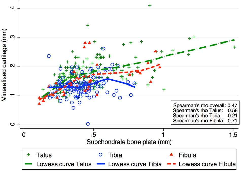
Scatterplot 1: Correlation between thickness of SBP and MC in the talar dome, the tibial plafond and the distal fibula, calculation of Spearman’s rho, and illustration by bone-specific lowess curves.

Figure 8.

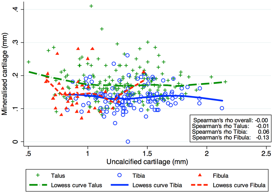
Scatterplot 2: Correlation between thickness of UC and MC in the talar dome, the tibial plafond and the distal fibula, calculation of Spearman’s rho, and illustration by bone-specific lowess curves.

Talus

Graphical regional distribution of SBP and MC showed in 13 of 20 (SBP) and in 7 of 20 (MC) ankle pairs, respectively, a symmetrical monocentric distribution pattern with highest SBP and MC values anteriorly or central medially. Only in 2 (SBP) and in 3 (MC) ankle pairs, respectively, a symmetrical bicentric distribution pattern was found with peaks of SBP and MC both medially and laterally, located in the anterior half of the talar dome (regions 1 and 4, as well as 3 and 6). Five (SBP) and 10 (MC) ankle pairs, respectively, could not be strictly assigned to 1 of the 2 patterns and showed 1 monocentric and 1 bicentric pattern per ankle. Histological median SBP and MC in the talar dome ranged from 0.30 to 0.66 mm and from 0.14 to 0.21 mm, respectively (Figure 4). Analogous to the findings in cartilage thickness measurements, a tendency of decreasing SBP values from medial to lateral could be identified.

Distal tibia and fibula

Histological median SBP and MC in the tibial plafond ranged from 0.35 to 0.53 mm and from 0.11 to 1.14 mm, respectively (Figure 6). Highest values were found in region 13 (posteromedially). In the distal fibula, MC and SBP values were in between the median range for the entire ankle joint. Median MC was 0.14 mm and 0.15 mm, respectively, and median SBP was 0.45 mm and 0.41 mm, respectively, in the proximal and distal fibular regions 16 and 17.

Cartilage indentation stiffness

Overall, inverse correlation was found between UC and CIS (Spearman’s rho overall −0.52) as well as between CT and CIS (Spearman’s rho overall −0.37) for the talar dome, the tibial plafond, and the distal fibula (Figure 9). This finding seemed to be even more evident in the range from 0.8 to 1.4 mm, where the majority of values were situated. Unequivocal correlation was identified neither between CIS and MC (Spearman’s rho overall 0.15) nor between CIS and SBP (Spearman’s rho overall −0.08). Median CIS value was 0.90N (range, 0.74 to 1.38) for the entire ankle joint.

Figure 9.

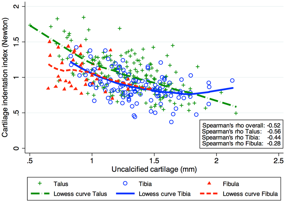
Scatterplot 3: Correlation between thickness of UC and cartilage indentation stiffness (CIS) in the talar dome, the tibial plafond and the distal fibula, calculation of Spearman’s rho, and illustration by bone-specific lowess curves.

Talus

CIS measurements showed in contrast to UC, CT, MC, and SBP in 14 of the 20 ankle pairs a bicentric distribution pattern with peak values concentrated at the anteromedial and anterolateral regions of the talar dome (Figure 10). Only in 3 ankle pairs was a symmetrical monocentric distribution pattern found, and 3 ankle pairs could not be strictly assigned to 1 of the 2 patterns. The values ranged from 0.84 to 1.28N (Figure 11).

Figure 10.

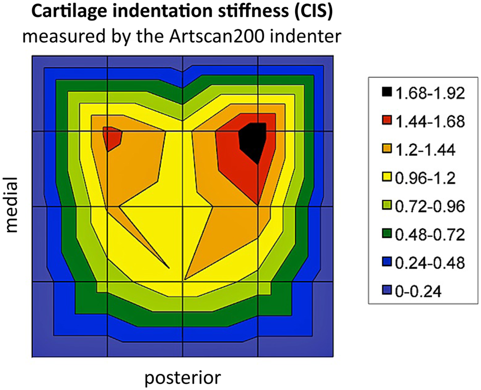
Example of a bicentric pattern of regional CIS distribution in the talar dome represented in color steps of 0.14 Newton (N), black 1.68 to 1.82N, dark green 0.48 to 0.72N.

Figure 11.

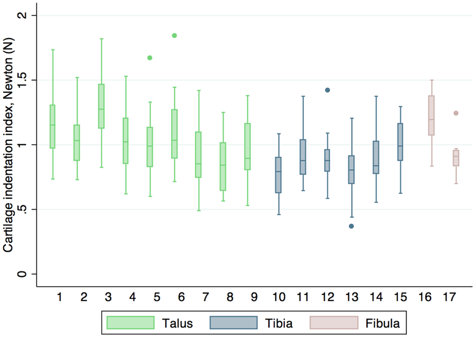
Box plot 3: Illustration of cartilage indentation stiffness distribution in Newton (N) for the talar dome in green (regions 1 to 9), the tibial plafond in blue (regions 10 to 15) and the distal fibula in red (regions 16 and 17), following the grid scheme.

Distal tibia and fibula

Median CIS values in the distal tibia ranged from 0.79 to 0.99N and were more uniformly distributed than those at the talar dome (Figure 11). There was a tendency that CIS was lower in the medial regions 10 and 13 than in the central and lateral regions 11 and 14, as well as 12 and 15. Broad differences were found in the fibula between the proximal (1.20N [IQR, 1.07-1.38]) and distal region (0.91N [IQR, 0.83-0.96]).

Discussion

This study provides a conclusive histological and biomechanical mapping of the regional morphometry of all 3 layers (UC, MC, SBP) that together form the osteochondral unit in the ankle joint. To our knowledge, there is no study available providing such insights and including a larger number of ankle pairs.

With regard to our first hypothesis, that the thickness of the SBP, its layer of MC, and the articular hyaline UC vary according to the localization within the human ankle joint, we found the histological articular hyaline UC thickness and SBP thickness showed clear regional differences. Cartilage thickness was highest at the mid and posterior talar dome, as well as at the tibial plafond. It was lowest in the anterior talus (regions 1-3) and the distal fibula. Interestingly, for both the talar dome and the tibial plafond, values at the regions close to the medial malleolus were higher than values at the lateral sides toward the fibula. These findings are mostly in accordance with results of previous studies on ankle joint cartilage thickness.^1,3,23,36,38 The little differences (on average +/− 0.2 mm) of the mean values in the abovementioned studies to the median values found in our study could be explained by technical details, that is, sample size, measurement techniques (ultrasound transducer,¹ sharp-needle transducer,^3,39 high-resonance x-ray,³⁸ high-resolution stereophophotography²³) and storage techniques of the specimens (fresh vs fresh frozen cadavers). Nevertheless, it has to be noted that differences in summary statistics (ie, calculations of mean and median values, respectively) can lead to substantial differences, especially in case of small sample sizes, making comparison difficult.

Histological thickness of the layer of MC and the SBP also varied strongly according to the localization within the human ankle joint. At the talus, MC and SBP were highest anteromedially and lowest posterolaterally. For the tibial plafond and the distal fibula, the values were more homogenously distributed. SBP was augmented only in the posteromedial region of the tibial plafond.

With regard to our second hypothesis, that the thickness of the articular hyaline UC at the talar shoulders is higher than the one at the talus center, we found the relevance of CT arthrography was its capacity for computerized reconstruction of reformatted planes, allowing visualization and measurement of the ankle specimens in the sagittal and coronal plane. It is noteworthy that in our study the anatomical finding of higher cartilage thickness at the talar shoulders^23,38 could be confirmed in the analysis of CT arthrography data.

In contrast to this finding, no second cartilage thickness peak over the lateral talar dome edge could be demonstrated by histomorphometry in our study. These differences were presumably due to technical particularities in our study, in fact, as a result of the placement of the histological sections directly in the center of each grid scheme region and not directly over the talar dome edges.

Sugimoto et al (high-resonance x-ray analysis on 29 ankles) focused on identifying cartilage thickness at the mid talar dome (corresponding to regions 4, 5, 6 in our study) in a coronal plane.³⁸ They found the thickest cartilage at both the medial and lateral talar dome edges, whereas—in conformity with our findings—values medially were higher than laterally. Millington et al performed high-resolution stereophotography before and after dissolving the articular cartilage in a sodium hypochlorite solution and was able to generate a 3-D geometric model of the ankle joint.²³ In his small series (12 ankle specimens), the highest cartilage thickness values were found anterolaterally and posteromedially over the talar dome edges. The value of multidetector row double-contrast CT arthrography in measurement of ankle cartilage thickness in comparison to MRI was evaluated by El-Khoury and Saltzman.⁹ They compared accuracy of both imaging techniques with histological measurement in 5 cadaveric ankles. Performance of double-contrast CT arthrography was considerably better.

Differences in overall cartilage thickness measured by CT arthrography and histomorphometry seem to derive from technical aspects of cartilage imaging. Exact differentiation of the borders to the joint space, filled by radiopaque dye on 1 hand, and the layer of subchondral bone on the other hand is difficult, due to limitations of resolution capacity. This apparently led to underestimation of articular cartilage thickness by CT arthrography. Interestingly, there was also a tendency in the study of El-Khoury and Saltzman toward underestimation of physical cartilage thickness by CT arthrography.⁹

With regard to our third hypothesis, that the cartilage stiffness in the human ankle joint varies according to the localization and is inversely correlated to cartilage thickness, we found that in the ankle joint cartilage stiffness was clearly inversely correlated to cartilage thickness.

Ankle cartilage is stiffer than cartilage at the knee or hip joint.^15,35,40 This is probably due to its special micro-molecular composition, with higher sulfated glycosaminoglycan content and lower water content.⁴¹ Indentation stiffness measurements showed inverse correlation with UC and CT arthrography cartilage thickness, meaning that CIS was higher in regions of thin hyaline UC. This finding confirms results in the literature published by Shepherd and others.^3,36,41 In the ankle joint, thin cartilage was mainly located at the anterior talar dome, exactly the region with the highest intrinsic joint stability when loaded in dorsiflexion. This finding fits the theory that soft cartilage is mainly found in low congruent joints with high peak stress loading, as present in the tibial plateaus or the patella surface, whereas rigid cartilage is seen in more congruent joints.^20,36,41

For the actual study, the optimized spherical-ended indenter for thin cartilage (< 2 mm) was used, to exclude bias due to interactions by small cartilage thickness.^14,21,22 The accuracy and reliability of handheld dynamic indentation probes in comparison with conventional indentation stiffness measurement apparatus have been confirmed by many authors.^2,18-20

With indentation stiffness measurement using the handheld Artscan200, we aimed to provide researchers and clinicians average values of intact ankle cartilage stiffness, as found in our series of 20 pairs of ankle joints. Comparison with arthroscopic cartilage stiffness of damaged ankle cartilage could be worthy of further investigation, making the Artscan a valuable diagnostic tool in ankle arthroscopy.

Interestingly, the majority of the specimens showed a bicentric distribution pattern regarding CIS, whereas for the SBP only a few of the specimens showed a bicentric distribution. Cartilage thickness was mainly monocentrically distributed. These results are partially in accordance with earlier findings, where the existence of a monocentric and a bicentric distribution type was demonstrated in a CT osteoabsorptionmetry study on the mineralization of the SBP of 34 ankle specimens.⁴⁵

Correlation analysis between the SBP, the MC and the articular UC showed that measurements of MC in the present study interestingly showed no correlation with the thickness of the hyaline UC. Such correlation has been suggested in former studies by our group,^26,27 in which it could be shown on different joints of the lower limb that, in areas of thick articular cartilage, the layer of the MC was also thickened. This could be seen in contradiction to our findings, at least regarding the human ankle. But it also could be taken as further evidence of specific anatomical and biomechanical requirements in the ankle as a primarily rolling joint with congruent surfaces, making different regional adaptations of UC, MC and SBP to loading necessary. The fact that the SBP in arthritic ankles does not show any increase in density, as found in other joints, may help in confirming this hypothesis.²⁵ However, strong positive correlation of MC to SBP thickness could be demonstrated for the talus, signaling coherent adaptations to regional loading. It is noteworthy that the median values of all 17 regions for the layer of MC ranged between 0.11 and 0.21 mm in our study and were surprisingly close to the values found by Wang et al for the femoral condyles of 40 human specimens (mean 0.104 mm).⁴⁴

A methodological shortcoming of this study could be seen in the relatively high median age of 78 years of the specimens. This is due to the fact that all cadaveric ankle joints were freshly obtained from donors of the affiliated pathologic institute of our university hospital. The specimens were stored in normal Saline at 4°C until fixation for histology. Time from harvest to fixation was not longer than 26 hours in any of the specimens in our series. The authors wanted to avoid the use of deep frozen cadaveric specimens that were thawed before the measurements. Obtaining fresh specimens of a younger cohort of donors—representing the typical age when osteochondral lesions occur—would not have been practical in our study setting. Theoretically, it cannot be categorically excluded that swelling or shrinking of the specimens by deep freezing and thawing could be a possible explanation for the differences seen in the different studies on ankle cartilage thickness cited above,^1,23,36,38 even though literature is available confirming that temporary freezing of specimens does not influence shape, size and content of the bone-cartilage units.²⁴

Although no or only minimal cartilage degeneration (according to ICRS and OARSI criteria) was found in our series, age-related differences between an older population (like ours) and a younger population as seen in a typical orthopedic practice cannot be excluded. Adam’s and Shepherd’s studies showed no significant negative correlation between age and thickness of articular hyaline cartilage.^1,36 Bae et al demonstrated early changes in indentation stiffness of early cartilage degeneration in the femoral condyle, whereas for macroscopically normal samples indentation stiffness scores did not depend on age of the donors.⁴ In a study on 1033 knee and ankle joints, 80% of the tali appeared grossly normal in a Collins scale and in the majority of cases normal ankle joints could be found even in advanced age.¹⁶ Ankle cartilage is less susceptible to osteoarthritic changes as seen in other joints and seems to stay in a relatively healthy condition also in elderly people⁶ due to a plethora of different degeneration protective factors.¹⁷ Replication of the tidemark and increase of SBP density, for example, is a well-known phenomenon with increasing age in knee and hip joints,^25,33,44 but was not detected in our series on ankle joints. Anyway, there are too little specific data available in the literature on early cartilage and subchondral bone alterations in the ankle joint of young patients. Our series did not allow age related subgroup analysis. Therefore, the median values for CIS and for the different components of the osteochondral unit in the ankle joint should only be transferred with precaution to a clinical setting where osteochondral lesions are surgically treated on teenagers. Noteworthy is that the correlation of thickness of the articular cartilage to body height and body weight could be found, potentially explaining gender differences.^1,3,36

Conclusion

In conclusion, the authors believe that this study contributes to knowledge of the specific properties of ankle joint osteochondral anatomy. These findings may improve understanding of the specific demands on operative restoration of ankle joint osteochondral lesions. Depending on their localization in the ankle joint, osteochondral plugs with an accurately fitting composition of cartilage thickness and stiffness, as well as of the SBP, may need to be transplanted to fulfill the specific histoanatomical and biomechanical regional requirements. Hence, a possible outcome of this study lies in the acknowledgment of important biomechanical limitations of transplanting osteochondral grafts from other joints. The information from this study might also promote research for optimized tissue-engineered osteochondral grafts, specially designed to replace focal osteochondral defects of the ankle.

Footnotes

Declaration of Conflicting Interests

The author(s) declared no potential conflicts of interest with respect to the research, authorship, and/or publication of this article.

Funding

The author(s) disclosed receipt of the following financial support for the research, authorship, and/or publication of this article: Supported by a grant from the American Orthopedic Foot & Ankle Society with funding from the Orthopedic Foot & Ankle Outreach & Education Fund (OEF) and the Orthopedic Research and Education Foundation (OREF).

References

Adam

Eckstein

Milz

. The distribution of cartilage thickness within the joints of the lower limb of elderly individuals. J Anat. 1998;193(pt 2):203-214.

Appleyard

Swain

Khanna

. The accuracy and reliability of a novel handheld dynamic indentation probe for analysing articular cartilage. Phys Med Biol. 2001;46:541-550.

Athanasiou

Niederauer

Schenck

Jr.

Biomechanical topography of human ankle cartilage. Ann Biomed Eng. 1995;23:697-704.

Bae

Temple

Amiel

. Indentation testing of human cartilage: sensitivity to articular surface degeneration. Arthritis Rheum. 2003;48:3382-3394.

Canale

Belding

. Osteochondral lesions of the talus. J Bone Joint Surg Am. 1980;62:97-102.

Cole

Margulis

Kuettner

. Distinguishing ankle and knee articular cartilage. Foot Ankle Clin. 2003;8:305-316.

Demetriades

Strauss

Gallina

. Osteoarthritis of the ankle. Clin Orthop Relat Res. 1998;349:28-42.

Duncan

Jundt

Riddle

. The tibial subchondral plate: a scanning electron microscopic study. J Bone Joint Surg Am. 1987;69:1212-1220.

El-Khoury

Alliman

Lundberg

. Cartilage thickness in cadaveric ankles: measurement with double-contrast multi-detector row CT arthrography versus MR imaging. Radiology. 2004;233:768-773.

10.

Elias

Zoga

Morrison

. Osteochondral lesions of the talus: localization and morphologic data from 424 patients using a novel anatomical grid scheme. Foot Ankle Int. 2007;28:154-161.

11.

Erben

. Embedding of bone samples in methylmethacrylate: an improved method suitable for bone histomorphometry, histochemistry, and immunohistochemistry. J Histochem Cytochem. 1997;45:307-313.

12.

Gobbi

Nunag

Malinowski

. Treatment of full thickness chondral lesions of the knee with microfracture in a group of athletes. Knee Surg Sports Traumatol Arthrosc. 2005;13:213-221.

13.

Hangody

Feczko

Bartha

. Mosaicplasty for the treatment of articular defects of the knee and ankle. Clin Orthop Relat Res. 2001;391:S328-S336.

14.

Hayes

Keer

Herrmann

. A mathematical analysis for indentation tests of articular cartilage. J Biomech. 1972;5:541-551.

15.

Kempson

. Age-related changes in the tensile properties of human articular cartilage: a comparative study between the femoral head of the hip joint and the talus of the ankle joint. Biochim Biophys Acta. 1991;1075:223-230.

16.

Koepp

Eger

Muehleman

. Prevalence of articular cartilage degeneration in the ankle and knee joints of human organ donors. J Orthop Sci. 1999;4:407-412.

17.

Kuettner

Cole

. Cartilage degeneration in different human joints. Osteoarthritis Cartilage. 2005;13:93-103.

18.

Laasanen

Toyras

Hirvonen

. Novel mechano-acoustic technique and instrument for diagnosis of cartilage degeneration. Physiol Meas. 2002;23:491-503.

19.

Lyyra

Jurvelin

Pitkanen

. Indentation instrument for the measurement of cartilage stiffness under arthroscopic control. Med Eng Phys. 1995;17:395-399.

20.

Lyyra

Kiviranta

Vaatainen

. In vivo characterization of indentation stiffness of articular cartilage in the normal human knee. J Biomed Mater Res. 1999;48:482-487.

21.

Lyyra-Laitinen

Niinimaki

Toyras

. Optimization of the arthroscopic indentation instrument for the measurement of thin cartilage stiffness. Phys Med Biol. 1999;44:2511-2524.

22.

Mak

Lai

Mow

. Biphasic indentation of articular cartilage—I. Theoretical analysis. J Biomech. 1987;20:703-714.

23.

Millington

Grabner

Wozelka

. Quantification of ankle articular cartilage topography and thickness using a high resolution stereophotography system. Osteoarthritis Cartilage. 2007;15:205-211.

24.

Milz

Putz

. Quantitative morphology of the subchondral plate of the tibial plateau. J Anat. 1994;185(pt 1):103-110.

25.

Muehleman

Berzins

Koepp

. Bone density of the human talus does not increase with the cartilage degeneration score. Anat Rec. 2002;266:81-86.

26.

Muller-Gerbl

Schulte

Putz

. The thickness of the calcified layer in different joints of a single individual. Acta Morphol Neerl Scand. 1987;25:41-49.

27.

Muller-Gerbl

Schulte

Putz

. The thickness of the calcified layer of articular cartilage: a function of the load supported? J Anat. 1987;154:103-111.

28.

O’Loughlin

Heyworth

Kennedy

. Current concepts in the diagnosis and treatment of osteochondral lesions of the ankle. Am J Sports Med. 2010;38:392-404.

29.

Outerbridge RE: The etiology of chondromalacia patellae. J Bone Joint Surg Br. 1961;43B:752-757.

30.

Pastoureau

Chomel

. Methods for cartilage and subchondral bone histomorphometry. Methods Mol Med. 2004;101:79-91.

31.

Peterson

Minas

Brittberg

. Two- to 9-year outcome after autologous chondrocyte transplantation of the knee. Clin Orthop Relat Res. 2000;374:212-234.

32.

Pritzker

Gay

Jimenez

. Osteoarthritis cartilage histopathology: grading and staging. Osteoarthritis Cartilage. 2006;14:13-29.

33.

Revell

Pirie

Amir

. Metabolic activity in the calcified zone of cartilage: observations on tetracycline labelled articular cartilage in human osteoarthritic hips. Rheumatol Int. 1990;10:143-147.

34.

Saltzman

Salamon

Blanchard

. Epidemiology of ankle arthritis: report of a consecutive series of 639 patients from a tertiary orthopaedic center. Iowa Orthop J. 2005;25:44-46.

35.

Shepherd

Seedhom

. The “instantaneous” compressive modulus of human articular cartilage in joints of the lower limb. Rheumatology (Oxford). 1999;38:124-132.

36.

Shepherd

Seedhom

. Thickness of human articular cartilage in joints of the lower limb. Ann Rheum Dis. 1999;58:27-34.

37.

Steadman

Rodkey

Rodrigo

. Microfracture: surgical technique and rehabilitation to treat chondral defects. Clin Orthop Relat Res. 2001;391:S362-S369.

38.

Sugimoto

Takakura

Tohno

. Cartilage thickness of the talar dome. Arthroscopy. 2005;21:401-404.

39.

Swann

Seedhom

. Improved techniques for measuring the indentation and thickness of articular cartilage. Proc Inst Mech Eng H. 1989;203:143-150.

40.

Swann

Seedhom

. The stiffness of normal articular cartilage and the predominant acting stress levels: implications for the aetiology of osteoarthrosis. Br J Rheumatol. 1993;32:16-25.

41.

Treppo

Koepp

Quan

. Comparison of biomechanical and biochemical properties of cartilage from human knee and ankle pairs. J Orthop Res. 2000;18:739-748.

42.

Valderrabano

Leumann

Rasch

. Knee-to-ankle mosaicplasty for the treatment of osteochondral lesions of the ankle joint. Am J Sports Med. 2009;37(suppl 1):105S-111S.

43.

van Dijk

Reilingh

Zengerink

. Osteochondral defects in the ankle: why painful? Knee Surg Sports Traumatol Arthrosc. 2010;18:570-580.

44.

Wang

Ying

Duan

. Histomorphometric analysis of adult articular calcified cartilage zone. J Struct Biol. 2009;168:359-365.

45.

Weileder

. Die “Physiologische Inkongruenz” des oberen Sprunggelenkes—ein optimiertes biologisches Bauprinzip auch in nicht-sphärischen Gelenken? Anatomische Anstalt Lehrstuhl I Munich, Ludwigs-Maximilians-Universität München, 67.