A fractional-order tempered-stable continuity model to capture surface water runoff

Abstract

The dynamics of surface runoff exhibits scale-dependent anomalous behavior due to heterogeneity present within natural systems, including spatial variations in surface topography and soil hydraulic properties which may not be efficiently captured by traditional modeling approaches. This study proposes a fractional-order continuity equation to quantify the scale-dependent anomalous behavior of overland flow, where the influence of sub-scale heterogeneity on flow dynamics can be characterized using spatiotemporally nonlocal terms built upon fractional derivatives. Both Eulerian and Lagrangian solvers are developed and cross-verified to approximate the proposed physical model. Numerical experiments further show that, on one hand, the space-fractional diffusive term in the flow model does not lead to apparent early arrivals in the steep rising limb of a hydrograph. This is likely caused by the combined effects of uniformly distributed precipitation over the entire hillslope and the immediate arrival of surface runoff at the downslope portion of the hillslope, both of which can overshadow the leading front of superdiffusion. The time-fractional term in the model, on the other hand, can 1) distinguish mobile and immobile water packets, 2) account for the strong time-nonlocal influence of net recharge on the receding limb of a hydrograph, and 3) efficiently characterize a wide range of late-time behavior of flow according to the tempered stable law. The applicability of the physical model is tested using two local-scale surface runoff data sets. The fractional-order tempered-stable flow model therefore may capture the complex hydrological response to precipitation in the real-world land surface.

Keywords

Fractional model tempered stable surface runoff anomalous diffusion

1. Introduction

Surface runoff (sometimes also called the overland flow) is a fundamental hydrological process that can affect other processes in morphology, biology, and ecology. Surface runoff, caused by infiltration or saturation excess overland flow, can lead to environmental (i.e. nonpoint source pollution and water sustainability) (Sedlak et al., 1997; Carpenter et al., 1998), agricultural (i.e. reduction of crop productivity due to soil conservation) (Kateb et al., 2013), and natural hazard issues (i.e. urban flooding) (Schmitt et al., 2004; Kabiri et al., 2013). For example, once surface runoff occurs, it can initiate other hydrological and ecological consequences. Torrential floods are the result of significant surface runoff generation. Surface runoff is also the main driving force for soil erosion, and may trigger debris flow hazards. It also redistributes water resources that may affect habitats and ecosystem in watersheds, and rapidly transports nutrients or contaminants within landscapes which affects multiple biological and ecological processes. Understanding the dynamics of surface runoff is therefore practically important and advances in understanding the dynamics of surface runoff provide benefits to numerous natural science disciplines.

Accurate quantification of surface runoff has remained a challenge in hydrology for many decades, as reviewed by Beven (2001). Many factors can affect the dynamics of surface runoff in natural systems, including topography, soil hydraulic properties, rainfall, and land cover, which may contain multi-scale intrinsic heterogeneity in both space and time (Chen et al., 2013). Surface runoff can therefore be viewed as a random process whose characteristics tend to evolve across scales. For example overland flow consists of both channeling, fast flow and separated, delayed water packets at the local scale, resulting in complex hydrographs (Mueller et al., 2007; Gomi et al., 2008). Most conventional hydrologic transport models, such as the popular ones solving the simplified Saint Venant equations of continuity and momentum, are either deterministic or physically based models that have well-known limitations in capturing the nuance of the runoff process across scales, including the apparent early arrivals and the delayed response in the hydrograph (see for example Rinaldo and Rodriguez-Iturbe, 1996).

The fractional engine has been found to be efficient in quantifying anomalous transport in heterogeneous systems that exhibit scale-dependency in medium properties (Metzler and Klafter, 2000), including natural soils (Zhang et al., 2009). This finding motivated us to develop fractional-derivative models to capture the anomalous flow of water, which is conceptualized in this study as the motion of water ‘packets’ along the land surface. In Section 2, we analyze the random nature of the surface runoff process, briefly review standard modeling approaches, and then propose a novel physical model and develop numerical solvers. The fractional-order flow model is applied to explore the response to various rainfall events in Section 3, and one real case is shown in Section 4. Late-time behavior of hydrographs is also analyzed for details. Possible future extensions of the physical model are then discussed in Section 5. Conclusions are provided in Section 6.

2. Methodology development

The first step of the current study is to define and analyze the hydrologic factors dominating surface runoff. This enables us to form a conceptual framework to develop the nonlocal, fractional-order model of overland flow proposed in this section.

2.1. Randomness in the surface runoff process

Topography may be one of the most important factors controlling surface runoff. At landscape scales, the overland flow surface varies with the undulating topography. Surface runoff tends to concentrate into preferential flow paths consisting of rills, gullies, and/or channels. At smaller scales, surface runoff is affected by micro-topography such as local depressions or mounds, gravel and cobble, and rills and micro-channels. Therefore, surface topography at multiple scales can either decelerate the flow (by storing water in surface depressions, increasing flow roughness, or altering flow routing paths) or accelerate the flow (in naturally concentrated flow paths), which might be captured by adding the time or space fractional-derivative term in the flow equation (that will be shown below).

The intrinsic heterogeneity of soil properties is another major factor affecting surface runoff. Soils have spatially varying hydraulic properties that cause the infiltration process, and in turn, the runoff generation process, to be strongly nonuniform in space (Maxwell and Kollet, 2008).

Some other factors may engender additional randomness in the dynamics of surface runoff. For example, hillslope subsurface stormflow can play a key role in runoff generation (Wilcox et al., 2008), where the heterogeneous distribution of hydraulic properties leads to the development of low-conductivity zones and/or preferential flow channels. Vegetation coverage can also affect runoff, by for example intercepting the rain water and changing soil properties and surface roughness (e.g. Dunne et al., 1991; Descroix et al., 2001).

The observed runoff also exhibits discontinuities across the surface (Gomi et al., 2008). Such discontinuities have been observed not only laterally, but also along the direction of flow. Discontinuous flow patterns, combined with the strong influence of heterogeneity in topography and soil properties, generate complex dynamics of surface runoff that may not be captured efficiently by the conventional models discussed below.

To draw an intermediate conclusion, the random nature of surface runoff may be simplified as a random walk process, where the jump size and waiting time of water packets can exhibit various distributions corresponding to the complex heterogeneity of topography and soil properties. It is also noteworthy that high-resolution digital elevation models and remote sensing of soil properties are available at present for the development of process-based hydrologic models, but such information cannot lead directly to the statistics of moving water packets along the regional land surface. Parsimonious models such as the fractional-derivative ones proposed by this study with pre-assumed statistics for water particle dynamics may therefore be highly relevant for practical applications.

2.2. The standard flow model

Existing theories for surface runoff dynamics mainly include full dynamic wave, diffusion wave, and kinematic wave equations (KWEs) (Singh, 1996). Currently both one-dimensional (1D) and two-dimensional (2D) models have been applied to watershed modeling practices. The 1D equations are briefly summarized here to provide a comparison baseline with our proposed models in the next section.

The following 1D KWE is a transient flow continuity model describing the mass balance of overland flow with recharge (Deng et al., 2006):

\partial h \partial t + \partial (uh) \partial x = p - i

(1)

where h [L] denotes the water thickness, u [LT⁻¹] is the water flux (depending on h:

u (x) = 1 n h (x) 2 / 3 (S_{0}) 1 / 2

, where n is Manning's coefficient and S₀ denotes the topographic slope), p [LT⁻¹] is the rainfall rate, and i [LT⁻¹] is the infiltration rate. Equation (1) is a nonlinear PDE, which can be simplified to a linear PDE under specific assumptions (such as runoff over a sufficiently steep rectangular hillslope; see Beven, 1981). The standard KWE (1) is a commonly accepted approximation of the Saint Venant equation.

The above 1D model however has intrinsic limitations in capturing scale-dependent surface runoff. First, it lacks the inclusion of sub-scale heterogeneity (such as the micro-topography and variations in soil hydraulic properties) that can significantly affect the overall flow pattern, such as heavy-tailed hydrographs with a long stretched recession limb (Harman et al., 2010). Second, lateral flow patterns are ignored. When the 1D approach is used, the watershed is segmented into sub-basins connected by a channel network. Each sub-basin can be further divided into several planes contributing to a certain reach of a channel (e.g. KINEROS2 model). Conventional 1D numerical procedures are then applied to each plane or the whole sub-basin to simulate surface runoff routing. It therefore captures the longitudinal variability of the topography and the soil to a certain degree, but it cannot represent the lateral heterogeneity, that is, variation within a cross-section. Lateral variability, especially caused by the topography, is a major feature of surface runoff.

2.3. The fractional-derivative model

Using the operator decomposition approach (Meerschaert et al., 2008), we propose the following fractional-derivative flow model:

\partial h_{t} \partial t + β \partial γ, λ_{t} h_{t} \partial t γ, λ_{t} = - V \partial h_{t} \partial x + D \partial α, λ_{x} h_{t} \partial x α, λ_{x} + β \int_{0}^{t} e - λ_{t} τ γ τ - γ - 1 Γ (1 - γ) f (x, τ) d τ

(2)

where β [T^γ−1] is the fractional capacity coefficient, γ [dimensionless] is the time index (0 < γ < 1), λ_t [T⁻¹] is the truncation parameter in time, V is the average flow velocity, D [LT⁻²] is the effective dispersion coefficient (due to mechanical dispersion only), α [dimensionless] is the space index (1 < α < 2), λ_x [L⁻¹] is the truncation parameter in space, Γ() [dimensionless] is the Gamma function, and f(x,t) = p − i [LT⁻¹] denotes the net recharge rate. The second term on the left-hand side of 2 denotes the tempered-stable operator in time (Meerschaert et al., 2008)

\partial γ, λ_{t} F \partial t γ, λ_{t} = e - λ_{t} t \partial γ (e λ_{t} t F) \partial t γ - (λ_{t}) γ F

(3)

and the second term on the right-hand side of 2 denotes the tempered-stable operator in space

\partial α, λ_{x} F \partial x α, λ_{x} = [e - λ_{x} x \partial α (e λ_{x} x) \partial x α - α (λ_{x}) α - 1 \partial \partial x - (λ_{x}) α] F

(4)

where the Riemann–Liouville fractional derivative is used in both space and time.

Here h_t denotes the thickness of water packets at the total (i.e. mobile plus immobile) phase. For the mobile phase with the thickness h_m, the governing equation is

\partial h_{m} \partial t + β \partial γ, λ_{t} h_{m} \partial t γ, λ_{t} = - V \partial h_{m} \partial x + D \partial α, λ_{x} h_{m} \partial x α, λ_{x}

(5)

where the last term in 2 (representing the source located in the total phase) disappears.

The space fractional-derivative term in 2 and 5 captures the superdiffusive movement of water packets along preferential flow paths, while the time fractional-derivative term in these models describes delays in the motion of water packets arising from soil heterogeneity and local topography. The combination of the two processes may generate a broad range of dynamics evolving in scales, which will be checked in Section 3.

To explain the physical process underlying the above models, here we simplify model (2) for the case of λ_t → 0 and λ_x → 0:

\partial h_{t} \partial t + β \partial γ h_{t} \partial t γ = - V \partial h_{t} \partial x + D \partial α h_{t} \partial x α + β t - γ Γ (1 - γ) h_{0} (x)

(6)

where h₀(x) represents the initial condition. If the water thickness h_t is replaced by the chemical concentration, equation (6) becomes the standard fractional advection–dispersion equation (fADE) reviewed extensively by Zhang et al. (2009). The fADE models and/or their continuous-time random walk (CTRW) analogues have been widely used to quantify anomalous super-/sub-diffusive transport in heterogeneous, saturated media at all scales (see for example Benson et al., 2001; Scher et al., 2002; Berkowitz et al., 2006; among many others). Recently, Schumer et al. (2009) presented a phenomenological discussion of how the fADE may model anomalous transport at the Earth's surface. We expect that the extended model (2) may also be applicable for describing overland flow across a continuum of length scales.

The CTRW corresponding to 6 has a heavy-tailed waiting time distribution with long time asymptotic decline as w(t) ∼ t^1 − γ, where the exponent γ is also the order of the time fractional-derivative in model (6) (Metzler and Klafter, 2000), and the corresponding late-time transport (such as the receding limb of the hydrography or tracer breakthrough curve) exhibits a similar power-law decline rate. The physical interpretation of the heavy-tailed waiting time distribution is the multiple-rate mass exchange between the mobile phase (i.e. the moving water) and multiple, parallel immobile phases (such as the low-permeability zones with various sizes and effective hydraulic conductivities) in the natural land surface with intrinsic, multi-scale heterogeneity (Haggerty et al., 2000). For relatively ‘homogeneous’ media, the probability density function (PDF) of waiting times cannot be as heavy as power law. Therefore we introduced the temporal truncation parameter λ_t to model (2), to capture a wide spectrum of waiting time PDFs transferring gradually from power law to exponential. The influence of λ_t on runoff will be discussed further in Section 3.2.

The CTRW corresponding to 6 also exhibits a heavy-tailed jump size PDF P(x) ∼ x^− α for large jumps (where x > 0 represents downstream movement), where α is the same as the order of the space fractional-derivative. Hence the fast displacement of water packets, such as those along preferential flow paths, has a heavy-tailed distribution. To account for the finite dimension of a typical preferential flow path, we added the spatial truncation parameter λ_x, so that model (2) can capture a wide spectrum of displacement PDFs.

2.4. Numerical approximations

The fractional-derivative models (2) and (5) can be approximated using both Lagrangian and Eulerian approaches. The Lagrangian solver contains two major steps: one for motion in space, and the other for motion in time, which can be expressed by the following discrete Langevin equations:

x_{n} = x_{n - 1} + V d t + [- D d t \cos (π α 2)] 1 / α d S_{α, λ_{x}}

(7a)

t_{n} = t_{n - 1} + d t + [β d t \cos (π γ 2)] 1 / γ d S_{γ, λ_{t}}

(7b)

Here x_n is the position of a randomly selected water packet after n steps, and t_n is the time at which the water packet reaches x_n. The parameter dt is the pre-assigned time step, the tempered-stable random variable

{dS}_{α, λ_{x}}

denotes the nth dispersive displacement (which can be generated using the exponential rejection approach; Baeumer and Meerschaert, 2010), and the tempered-stable random variable

{dS}_{γ, λ_{t}}

is the immobile time prior to the nth jump. The space process (7a) accounts for the mean displacement due to both advection and the potential superdiffusion deviating from the mean (for example due to preferential flow paths) for water packets, while the time process (7b) records motion time dt and the time between transport events, presuming that transport is episodic as a result of both flow variations and local water storage. In addition, the source term in (2) can be approximated conveniently by injecting and tracking the recharging water packets. For the development of (7), we refer to the fractional-order adjoint method proposed in Zhang et al. (2006) and the time-Langevin approach in Zhang et al. (2008) for interested readers.

One example of particle trajectories generated by (7) is shown in Figure 1. For a small time step dt, the discrete jump at each individual step (see Figure 1(a)) looks more continuous (Figure 1(b)), and the resultant number density for particles exiting the downslope boundary can be converted to the volume of flow leaving the model domain per unit of time (i.e. the discharge). For demonstration purposes, Figure 1(a) and Figure 1(b) assume that the jump occurs instantaneously between two waiting events.

Figure 1.

(a) Discrete-time random walk for one particle representing one individual water packet flowing along land surface. (b) Continuous-time random walk and its evolution in time for 20 walkers. (c) The simulated cumulative mass using both the Lagrangian solver (symbols) and the Eulerian solver (line) for water packets exiting the downslope boundary. The model parameters (assumed to be dimensionless for simplicity) are as follows: α = 1.70, λ_x = 1 × 10⁻⁵, γ = 0.50, β = 0.1, λ_t = 1 × 10⁻⁵, V = 2, D = 0.2, and the travel distance L = 20.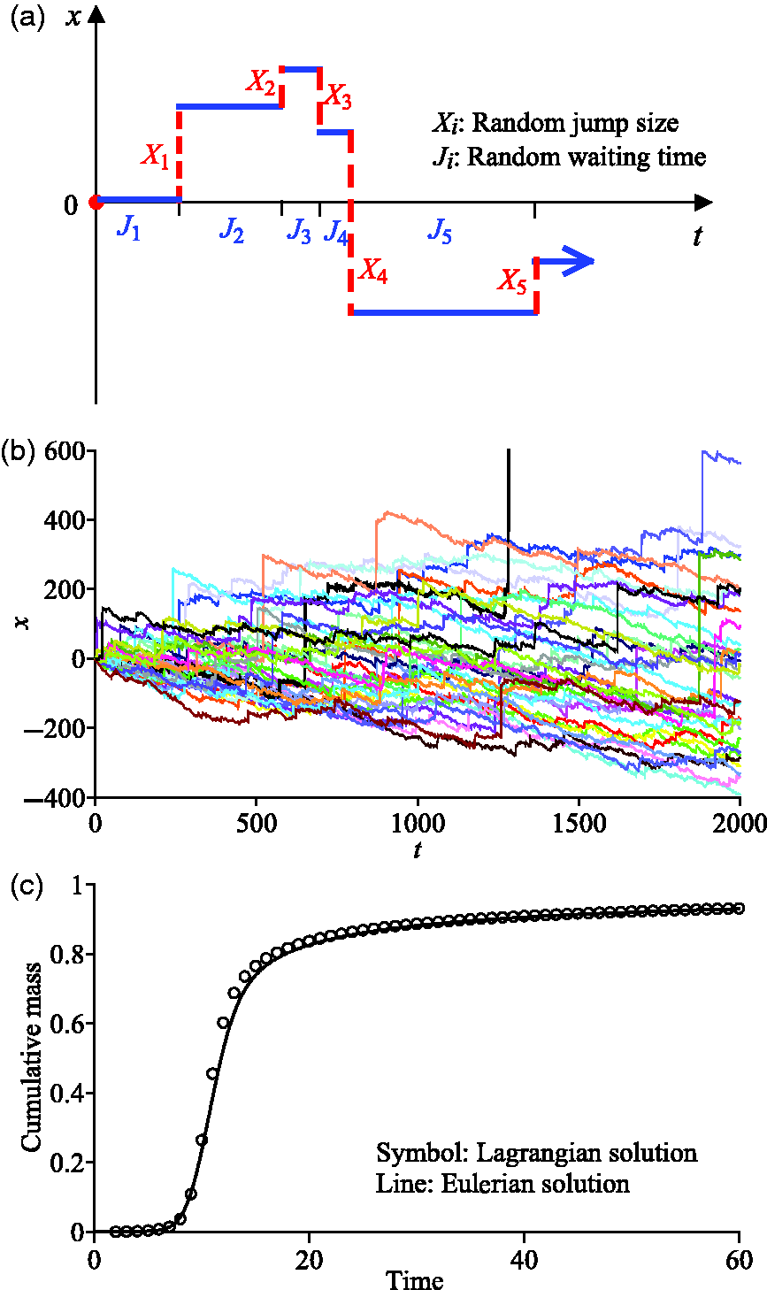

For the purpose of cross-verification, we also solve (2) using the Eulerian method. Equation 2 can be discretized using the implicit finite difference scheme (where the subscript ‘t’ of the water thickness h is ignored for description simplicity):

h_{i}^{n + 1} - h_{i}^{n} Δ t + β e - λ_{t} t_{n + 1} (Δ t) γ \sum_{k = 0}^{n + 1} [g_{k} e λ_{t} t_{n - (k - 1)} h_{i}^{n - (k - 1)}] - β (λ_{t}) γ h_{i}^{n + 1} = - V h_{i + 1}^{n + 1} - h_{i}^{n + 1} Δ x + D {e - λ_{x} x_{i} (Δ x) α \sum_{j = 0}^{i + 1} w_{j} e λ_{x} x_{i - (j - 1)} h_{i - (j - 1)}^{n + 1} - (λ_{x}) α h_{i}^{n + 1} - (λ_{x}) α - 1 α h_{i + 1}^{n + 1} - h_{i}^{n + 1} Δ x} + β \sum_{l = 1}^{n + 1} e - λ_{t} t_{l} f (x_{i}, t_{l}) Δ t (t_{l}) - γ Γ (1 - γ)

(8)

where g_k and w_j denote the Grünwald weight for the γ-order and α-order fractional derivative, respectively; and Δt and Δx are the step sizes in time and space, respectively.

Repeating 8 for each node, one can get the final equations

[A] h n + 1 = h n + Δ t S n + 1

(9)

where [A] is a (K + 1) × (K + 1) coefficient matrix; hⁿ⁺¹, hⁿ, and Sⁿ⁺¹ are (K + 1) vectors; and K + 1 denotes the total number of nodes in space.

The entry in [A] is

{AS}_{i, j} = {0 - \frac{Δ t}{(Δ x) α} D w_{0} e λ_{x} Δ x, 1 + \frac{β g_{0}}{(Δ t) γ - 1} - Δ t β (λ_{t}) γ + V η - B, - V η - η D [\frac{w_{2} e - λ_{x} Δ x}{(Δ x) α - 1} + α (λ_{x}) α - 1], - \frac{Δ t}{(Δ x) α} D w_{i - (j - 1)} e - λ_{x} (i - j) Δ x, j > i + 1 j = i + 1 j = i j = i - 1 j < i - 1

where η = Δt/Δx, B = ΔtD[w₁/(Δx)^α − (λ_x)^α − α (λ_x)^α−1/Δx]; A_0,0 = 1; A_0,j = 0 for j = 1, … , K; A_K,K = 1; A_K,K−1 = − 1; and A_K,j = 0 for j = 0, … , K − 2.

The Greschgorin theorem (Isaacson and Keller, 1966) is used to explore the stability of the above finite difference scheme. Results show that the Eulerian scheme is conditionally stable with the stability criterion of Δt < 1/λ_t. A similar discretization scheme and stability analysis can be conducted for equation 5.

Numerical tests show that the Eulerian solution generally matches the Lagrangian solution, with one example shown in Figure 1(c). This example contains an instantaneous source close to the upslope boundary. Water packets then begin to move downslope. The spatial distribution of the mobile phase thickness has a heavier leading front and a faster moving peak than the immobile phase (not shown here), as expected.

The above two solvers are quite different and have intrinsic advantages and disadvantages. The Lagrangian solver is grid-free and therefore can be computationally efficient (especially for small values of γ where water packets remain stagnant during most of the travel history), while the Eulerian solver compensates for the limitations of the Lagrangian solver in capturing the extremely low density at the tail of the hydrograph. Therefore no solver is apparently superior to the other for the flow models developed in this study, and both solvers are used in the generation of figures shown in the following section.

3. Numerical investigation of the surface runoff process

Here we analyze numerically the contribution of various terms in the flow model (2) to surface runoff. Such contributions may be related to hydrologic mechanisms, which will also be discussed below.

3.1. Impact of the nonlocal recharge term on surface runoff

The last term in 8 implies that rainfall should be a time-nonlocal term in the fractional-order flow model (2). In other words, the time variation of the water thickness (or actually the mass) at present is related to the historical load of net recharge at the same position. Not all of the precipitation reaching the ground can instantaneously exit the downgradient boundary. Due to the complex flow pattern, some water packets may extend laterally and/or be trapped by depressions before moving longitudinally. Such a time-nonlocal process significantly affects the tailing behavior of the hydrograph.

To reveal the impact of the source term on surface runoff dynamics, we first calculate the hydrograph by considering the ‘nonlocality of the recharge’. One example is shown in Figure 2 (the dashed line), where the hydrograph exhibits apparent late-time tailing due to the contribution from the previous recharge. We then re-calculate the flow process with ‘time-local recharge’, where the last term in 8 reduces to $β e - λ_{t} t_{n + 1} f (x_{i}, t_{n + 1}) Δ t (t_{n + 1}) - γ / Γ (1 - γ)$ . In this case, only the current rainfall can affect the current variation of water mass (i.e. memoryless). The resultant hydrograph contains a recession limb with a much greater rate of decline (see the black line in Figure 2). When the time index γ approaches 1 and the contribution of the initial source to runoff is simplified as a time-local term (which may represent a homogeneous system), the water discharge at the later time declines as fast as exponential (shown by the gray line in Figure 2), approaching its asymptote described by the standard KWE model.

Figure 2.

Computed water discharge using the fractional-order flow model, where the recharge has either the time-nonlocal effect or time-local effect. Two uniform rainfall events (denoted as f₁ and f₂, respectively) at times 2 ≤ t ≤ 3 and 30 ≤ t ≤ 32 (units: hours) are considered.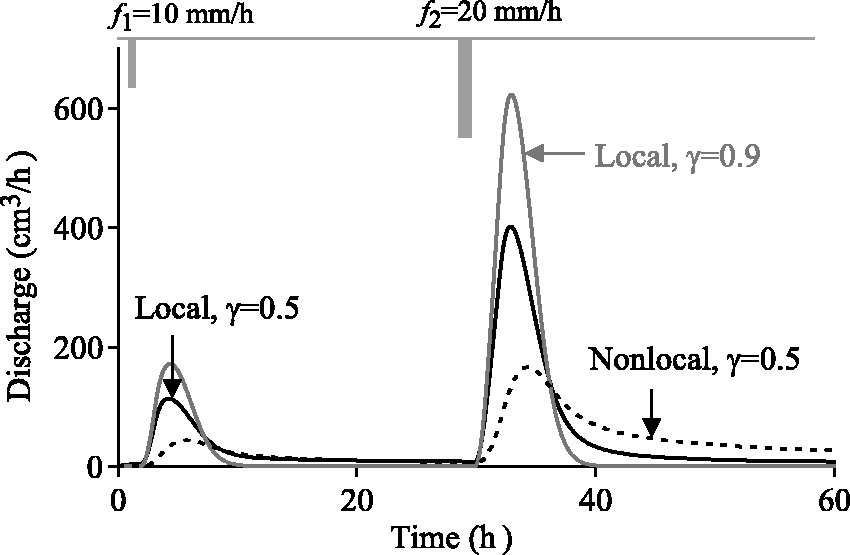

Many transport processes involve a source/sink term. Whether the source/sink term should remain a local term or be treated as a nonlocal term therefore is an important question when the time fractional-derivative replaces its integer-order counterpart; see for example, the various possible forms of the coupled reaction–subdiffusion model proposed in Henry et al. (2006). The above numerical tests reveal that the nonlocal source term elongates the late-time tail and decreases the peak discharge of the hydrograph. Thus, hydrograph characteristics of natural systems can likely be used to distinguish the locality of source/sink terms in (2).

3.2. Influence of the time fractional-derivative term

The time fractional-derivative term on the left-hand side of 2 controls the memory of flow response to recharge events. Numerical experiments show that the recession limb of the hydrograph is enhanced with the decrease of the time index γ (Figure 3(a)), an increase of the capacity coefficient β (Figure 3(b)), and/or the decrease of the truncation parameter λ_t (Figure 3(c)). This is expected, because a smaller γ defines a higher probability for long residence times, a larger β assigns a larger portion of immobile water packets, and a smaller λ_t leads to a later transition from power law to exponential decline of the waiting time PDF.

Figure 3.

Subdiffusion affected by the (a) scale index γ, (b) capacity coefficient β, and (c) truncation parameter λ_t: computed water discharge using the Eulerian solver. A single uniform rainfall event occurs at time 3 ≤ t ≤ 6 h.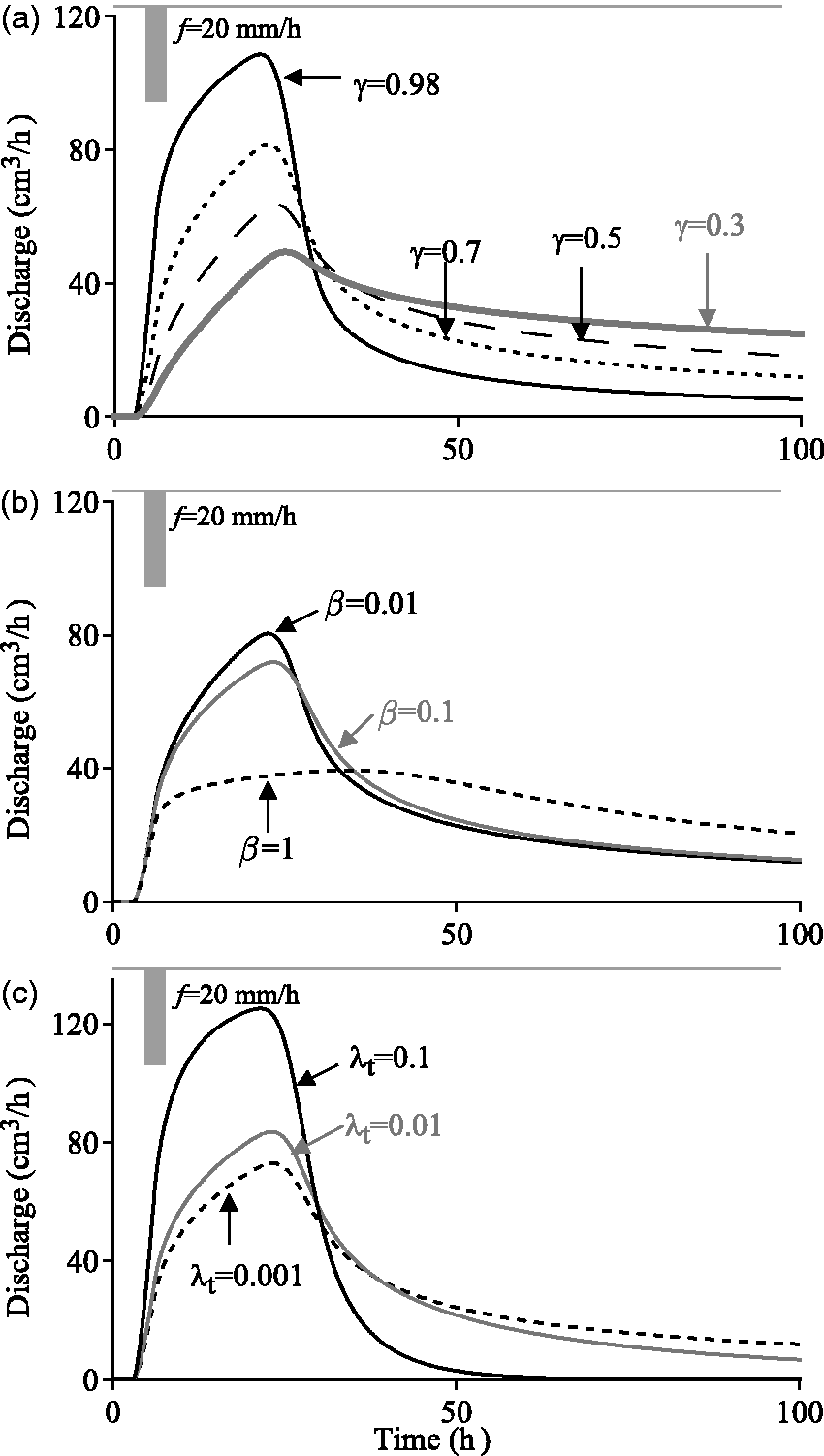

It is also noteworthy that, in an open system like the Earth's surface, a transport process can also exchange mass with surrounding media. At a very long time after the rainfall, water trapped by depressions may not contribute to the hydrograph, but rather infiltrate downward at a small rate or even evaporate back to the atmosphere. In other words, the recession limb may transition from a purely power-law tail to a faster decline rate in a typical real-world hydrograph. This can be inferred from the observed hydrograph shown in Rinaldo and Rodriguez-Iturbe (1996). A tempered stable model therefore may be practically more attractive than the standard stable model in quantifying the late-time dynamics of surface runoff.

3.3. The space nonlocality versus the time nonlocality

Although the competition between the space and time nonlocal processes can cause the complex scaling behavior for transport (Zhang et al., 2012), the superdiffusive movement does not alter the late-time decline of the hydrograph. As shown by Figure 4(a), the late-time tail of the calculated hydrograph decays as ∼t^−1−γ, for a small truncation parameter λ_t (representing the persistent power-law decline of long waiting times).

Figure 4.

(a) Subdiffusion affected by the scale index γ, with continuous and time-varying recharge f(t) on the whole slope (computed using the Lagrangian solver); α = 1.6 for all cases, and a small λ_t (=1 × 10⁻⁶ h⁻¹) is used. (b) Superdiffusion affected by the scale index α, with continuous and time-varying recharge f(t) on the whole slope; γ = 0.5 for all cases. (c) Computed water discharge using the Eulerian solver. One rainfall event occurs at time 3 ≤ t ≤ 6 h and recharges the upslope, and the time index γ = 0.9.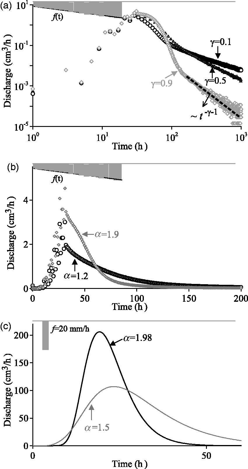

Superdiffusive motion of water packets captured by the space fractional-derivative term in 2 affects the rising limb of the hydrograph. For the case of a short recharge injected around the upslope boundary, the resultant hydrograph exhibits a heavier early tail for a smaller index α (Figure 4(c)), as expected. When the continuous rainfall uniformly covers the whole ground surface, however, there are no apparent early arrivals in the steep rising limb of the hydrograph (Figure 4(b)), probably due to the water packets exiting the downslope boundary immediately (which overshadows the leading front of superdiffusion).

The superdiffusive transport of water packets may also be interrupted by the discontinuous flow patterns discussed above. The length of natural preferential flow paths in soils should be much less than hundreds of meters (Beven and Germann, 2013), providing a natural cutoff for large displacement for water packets during one single jump. This is also the reason that the tempered stable model is selected to control particle jumps in this study.

4. A preliminary application of the physical model

Here we check the applicability of the above physical model against two local-scale experiments of surface runoff conducted by Deng et al. (2006) using a soil flume (where the flume bed had a slope of 10%) and a rainfall simulator. In their experiments, relatively uniform soils were used and the resultant soil surface was smooth (without rough elements such as micro-topographic protuberances). The length of water application to the soil surface along the slope was 5.3 m, and therefore this is a local scale process.

Applications show that the model (2) can match trends from the first experiment, hydrograph 1 (see the black line in Figure 5(a) and (b)). The normalized discharge is used, considering the unknown infiltration and evaporation. The best-fit model parameters are as follows: α = 2, γ = 0.775, β = 0.225 s^γ−1, and λ_t = 0.02 s⁻¹. On one hand, the space index α (where α = 2) implies Fickian diffusion for the fast moving water packets. This is expected, since 1) the flat soil surface cannot maintain interconnected preferential flow paths, and 2) the measured hydrograph does display a steep rising limb (note that the initial rainstorm did not cover the whole slope uniformly). On the other hand, the long-tailed distribution of the hydrograph can be efficiently captured by the parameters γ, β, and λ_t that define the trapping process. Even under the simplified conditions (i.e. relatively uniform soils and smooth surface) in this experiment, the flow velocity can vary along the soil surface (Deng et al., 2006) where the delayed flow forms the late-time tailing. It is also noteworthy that we observed similar late-time tailing behavior in tracer transport through relatively uniform and saturated soils repacked in sand columns (Zhang et al., 2014). To further check the sensitivity of the tailing behavior to model parameters, we add two more model results with γ = 0.80 and β = 0.30 s^γ−1 for model (1), and γ = 0.75 and β = 0.15 s^γ−1 for model (2) (see the gray and dashed lines in Figure 5(a) and (b)). Model (1) overestimates the hydrograph tail (since it assumes a larger capacity coefficient), while model (2) underestimates the tail (due to the smaller capacity coefficient). Therefore the nuance of the late-time tail of hydrographs can be captured by the time index and capacity coefficient.

Figure 5.

Applications of model (2): experimental data (symbols; from Deng et al., 2006) versus the model simulations (lines) for hydrograph 1 (a) and 2 (c). (b) and (d) are the log–log plots of (a) and (c), respectively, to show the tailing behavior.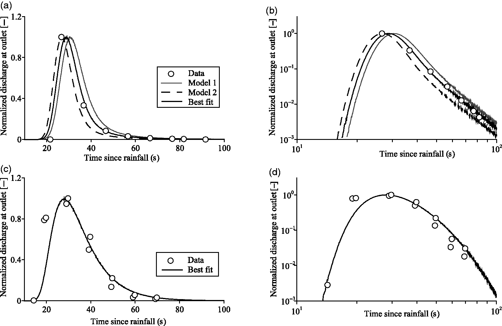

We then fit the second experimental data, where the rainfall moved along the slope in a different mode (Deng et al., 2006). Compared to the measurement in the first experiment, the second hydrograph contains a shorter late-time tail, but the overall rising and receding limbs have a wider expansion (see symbols in Figure 5(c) and (d)). Such a discrepancy can be characterized by model (2) using a relatively larger β (=1.025 s^γ−1) and λ_t (0.09 s⁻¹) and a relatively smaller γ (0.475).

The above preliminary application shows that the fractional-derivative model (2) may quantify the hillslope-scale runoff process. Whether it can capture a larger scale (such as the basin scale) process remains to be shown. Previous applications by hydrogeologists show that the fADE model is especially applicable for large aquifer/aquitard systems (Zhang et al., 2009), because the complex heterogeneity tends to favor the assumption of heavy-tailed waiting time and jump size PDFs. We will test the applicable scale for model (2) in a future study.

5. Discussion: future extensions of the physical model

The above tests show the fractional-derivative model (2) can describe key characteristics of surface runoff dynamics. Further possible extensions are needed to quantify additional complicated behaviors of real-world surface runoff.

First, before the runoff response becomes stable, the water flux can vary with water thickness and the travel time, as implied by u(h) in the KWE 1. The new flow model (2) assumes a mean velocity (since the fractional-derivative terms can capture the deviation from the mean advection in either space or time), which may miss the transient variation, especially in the rising limb of the hydrograph. To address this question, we will incorporate the above Lagrangian scheme in the widely used particle-tracking-based software RWHet (LaBolle, 2006) in a future study, where the velocity and dispersion coefficients are space- and time-dependent.

Second, water can also be removed at late times (due to infiltration/evaparation) during the surface runoff process, an impact that cannot be simulated directly by model (2). In this study, the source term f denotes the net recharge to surface runoff. The mobile/immobile separation however cannot explain any permanent mass loss during runoff, since the immobile particle will become mobile when exceeding the waiting time. To efficiently account for the possible mass loss, one may assign a decay rate for each immobile particle. When the particle becomes mobile again, part of the mass is lost due to ‘decay’. We will test this hypothesis in a future study.

Third, this study assumes that the land surface remains stationary, so that a constant dispersion coefficient D can be used. However, the diffusivity for some disordered systems, such as the heterogeneous porous media, can increase with the travel distance even when a fractional engine is used (Zhang et al., 2007). The disordered system may show weak ergodicity breaking, where the ensemble and time averaged quantities (such as the mean squared displacement of water packets) behave differently (Cherstvy et al., 2013; Massignan et al., 2014). Recently, Cherstvy et al. (2014) found that a Markovian stochastic process with a radially varying D efficiently describes nonergodic, anomalous diffusion. Massignan et al. (2014) found that random patch models provide an alternative for describing nonergodic diffusion in biological systems. To capture the potentially nonergodic anomalous surface runoff, the above approaches may be applied. In addition, one may also update D in model (2) with a space-variable D(x) (Zhang et al., 2007), or apply a mathematical tool called ‘subordination’ (Baeumer et al., 2001; Harman et al., 2010) where the displacement of water packets deviating from the mean velocity can be described by the random and space-dependent movement along streamlines. We will explore the above extensions in a future study.

6. Conclusion

The complex process of water flowing across a heterogeneous land surface can be simplified as a random walk process with independent particles representing water packets. The preferential flow paths that facilitate the rapid movement of water packets can be discontinuous and vary with scale, while depressional storage and complex horizontal flow patterns delay the longitudinal displacement of water. Such a stochastic process motivates the application of the fractional engine.

This study develops a new theoretical framework based on stable laws and builds nonlocal transport models for surface runoff to account for the impact of system heterogeneity (such as topography and soil properties) and scaling. Numerical methods are then developed to generate solutions to the governing equations and investigate the performance of the proposed model.

Numerical experiments show that the fractional-order tempered-stable flow model can capture several properties of surface runoff that may not be quantified efficiently by traditional models, including 1) the separation of mobile and immobile water packets, 2) the strong time-nonlocal influence of net recharge on the recession limb of the hydrograph, and 3) the various late-time tails (from power law to exponential distributions) of the hydrograph.

Footnotes

Funding

The authors are thankful for the financial support of the National Science Foundation (grant numbers DMS-1025417 and DMS-1460319) and the United States Geological Survey, State Water Research Institute Program (grant number 2013NV196B). This paper does not necessarily reflect the view of the funding agencies.

References

Baeumer

Meerschaert

(2010) Tempered stable Levy motion and transient super-diffusion. Journal of Computational and Applied Mathematics 233: 2438–2448.

Baeumer

Meerschaert

Benson

(2001) Subordinated advection-dispersion equation for contaminant transport. Water Resources Research 37: 1543–1550.

Benson

Schumer

Meerschaert

(2001) Fractional dispersion, Lévy motion, and the MADE tracer tests. Transport in Porous Media 42(1/2): 211–240.

Berkowitz

Cortis

Dentz

(2006) Modeling non-Fickian transport on geological formations as a continuous time random walk. Review of Geophysics 44(2): RG2003.

Beven

(1981) Kinematic subsurface stormflow. Water Resources Research 17(5): 1419–1424.

Beven

(2001) Rainfall-Runoff Modelling: The Primer, Chichester, UK: Wiley.

Beven

Germann

(2013) Macropores and water flow in soils revisited. Water Resources Research 49: 3071–3092.

Carpenter

Caraco

Correll

(1998) Nonpoint pollution of surface waters with phosphorus and nitrogen. Ecological Applications 8: 559–568.

Chen

Sela

Svoray

(2013) The role of soil-surface sealing, microtopography, and vegetation patches in rainfall-runoff processes in semiarid areas. Water Resources Research 49(9): 5585–5599.

10.

Cherstvy

Chechkin

Metzler

(2013) Anomalous diffusion and ergodicity breaking in heterogeneous diffusion processes. New Journal of Physics 15: 083039.

11.

Cherstvy

Chechkin

Metzler

(2014) Particle invasion, survival, and non-ergodicity in 2D diffusion processes with space-dependent diffusivity. Soft Matter 10: 1591–1601.

12.

Deng

de Lima

JLMP

de Lima

MIP

(2006) A fractional dispersion model for overland solute transport. Water Resources Research 42: W03416.

13.

Descroix

Viramontes

Vauclin

(2001) Influence of soil surface features and vegetation on runoff and erosion in the Western Sierra Madre (Durango, Northwest Mexico). Catena 43: 115–135.

14.

Dunne

Zhang

Aubry

(1991) Effects of rainfall, vegetation, and microtopography on infiltration and runoff. Water Resources Research 27(9): 2271–2285.

15.

Gomi

Sidle

Miyata

(2008) Dynamic runoff connectivity of overland flow on steep forested hillslopes: Scale effects and runoff transfer. Water Resources Research 44: W08411.

16.

Haggerty

McKenna

Meigs

(2000) On the late-time behavior of tracer test breakthrough curves. Water Resources Research 36: 3467–3479.

17.

Harman

Reeves

Baeumer

(2010) A subordinated kinematic wave equation for heavy-tailed flow responses from heterogeneous hillslopes. Journal of Geophysical Research 115: F00A08.

18.

Henry

Langlands

TAM

Wearne

(2006) Anomalous diffusion with linear reaction dynamics: From continuous time random walks to fractional reaction-diffusion equations. Physical Review E 74(3): 031116.

19.

Isaacson

Keller

(1966) Analysis of Numerical Methods, New York, NY: Wiley.

20.

Kabiri

Chen

Bai

(2013) Comparison of SCS and Green-Ampt methods in surface runoff-flooding simulation for Klang Watershed in Malaysia. Open Journal of Modern Hydrology 3(3): 102–114.

21.

Kateb

Zhang

(2013) Soil erosion and surface runoff on different vegetation covers and slope gradients: A field experiment in Southern Shanxi Province, China. Catena 105: 1–10.

22.

LaBolle

(2006) RWHet: Random walk particle model for simulating transport in heterogeneous permeable media, CA: User manual and program documentation, University of California.

23.

Massignan

Manzo

Torreno-Pina

(2014) Nonergodic subdiffusion from Brownian motion in an inhomogeneous medium. Physical Review Letters 112: 150603.

24.

Maxwell

Kollet

(2008) Quantifying the effects of three-dimensional subsurface heterogeneity on Hortonian runoff processes using a coupled numerical, stochastic approach. Advances in Water Resources 31(5): 807–817.

25.

Meerschaert

Zhang

Baeumer

(2008) Tempered anomalous diffusion in heterogeneous systems. Geophysical Research Letters 35: L17403.

26.

Metzler

Klafter

(2000) The random walk's guide to anomalous diffusion: A fractional dynamic approach. Physics Reports 339: 1–77.

27.

Mueller

Wainwright

Parsons

(2007) Impact of connectivity on the modeling of overland flow within semiarid shrubland environments. Water Resources Research 43: W09412.

28.

Rinaldo

Rodriguez-Iturbe

(1996) Geomorphological theory of the hydrological response. Hydrological Processes 10: 803–829.

29.

Scher

Margolin

Metzler

(2002) The dynamical foundation of fractal stream chemistry: The origin of extremely long retention times. Geophysical Research Letters 29(5): 1061.

30.

Schmitt

Thomas

Ettrich

(2004) Analysis and modeling of flooding in urban drainage systems. Journal of Hydrology 299(3–4): 300–311.

31.

Schumer

Meerschaert

Baeumer

(2009) Fractional advection-dispersion equations for modeling transport at the Earth surface. Journal of Geophysical Research 114: F00A07.

32.

Sedlak

Phinney

Bedsworth

(1997) Strongly complexed Cu and Ni in wastewater effluents and surface runoff. Environmental Science and Technology 31(10): 3010–3016.

33.

Singh

(1996) Kinematic Wave Modeling in Water Resources: Surface Water Hydrology, New York, NY: Wiley.

34.

Wilcox

Taucer

Munster

(2008) Subsurface stormflow is important in semiarid karst shrublands. Geophysical Research Letters 35(10): L10403.

35.

Zhang

Benson

Meerschaert

(2007) Space-fractional advection-dispersion equations with variable parameters: Diverse formulas, numerical solutions, and application to the Macrodispersion Experiment site data. Water Resources Research 43: W05439.

36.

Zhang

Benson

Meerschaert

(2006) On using random walks to solve the space-fractional advection-dispersion equations. Journal of Statistical Physics 123(1): 89–110.

37.

Zhang

Meerschaert

Baeumer

(2008) Particle tracking for time-fractional diffusion. Physical Review E 78: 036705.

38.

Zhang

Benson

Reeves

(2009) Time and space nonlocalities underlying fractional-derivative models: Distinction and literature review of field applications. Advances in Water Resources 32: 561–581.

39.

Zhang

Meerschaert

Packman

(2012) Linking fluvial bed sediment transport across scales. Geophysical Research Letters 39: L20404doi:10.1029/2012GL053476.

40.

Zhang

Qian

Papelis

(2014) Improved understanding of bimolecular reactions in deceptively simple homogeneous media: From laboratory experiments to Lagrangian quantification. Water Resources Research 50: 1704–1715.