Force identification under unknown initial conditions by using concomitant mapping matrix and sparse regularization

Abstract

Unknown initial conditions can affect the identified accuracy of dynamic forces. Direct measurement of initial conditions is relatively difficult. This study proposes a sparse regularization–based method for identifying forces considering influences of unknown initial conditions. The initial conditions are embedded in a classical governing equation of force identification. The key idea is to introduce a concept of concomitant mapping matrix for reasonably expressing the initial conditions. First, a dictionary is introduced for expanding the dynamic forces. Then, the concomitant mapping matrix is formulated by using free vibrating responses, which correspond to structural responses happening after the structure is subjected to each atom of the force dictionary. A sparse regularization strategy is applied for solving the ill-conditioned equation. After that, the problem of force identification is converted into an optimization problem, and it can be solved by using a one-step strategy. Numerical simulations are carried out for verifying the feasibility and effectiveness of the proposed method. Illustrated results clearly show the applicability and robustness of the proposed method for dealing with force reconstruction and moving force identification.

Keywords

Force identification sparse regularization concomitant mapping matrix unknown initial condition inverse problem

1. Introduction

Civil structures are one of the best carriers of socioeconomic development. The safety of civil structures has been widely concerned. The civil structures are often subjected to some dynamic forces during their lifetime. Collecting exact information of dynamic forces and structural parameters plays a positive role for ensuring the safety of civil structures (Jayalakshmi and Rao, 2017). Direct measurement and indirect identification are two common methods for measuring the dynamic forces. Herein, the indirect method means that the forces are reconstructed from some structural responses (Wang et al., 2019).

The force identification belongs to a classical inverse problem in the field of structural dynamics, and it has been widely studied for a long time. (Li et al., 2018; Prawin and Rama Mohan Rao, 2018; Sanchez and Benaroya, 2014; Zheng et al., 2019). According to whether structural nonlinear behavior is considered or not, existing force identification methods can fall into linear method or nonlinear method. For example, the compressed sensing-based method for moving force identification proposed by Liu et al. (2020) belongs to linear methods. Contrarily, the unscented Kalman filter–based method proposed by Guo et al. (2018) belongs to nonlinear methods because the structure considered in this work is nonlinear. Generally, researches and applications of linear methods are more common than the ones of nonlinear methods. The reason is obvious because a real structure is often designed to work within an elastic range during its normal service period. Furthermore, according to properties of the considered variables, linear force identification methods can be subdivided into two categories such as probabilistic/statistical method and deterministic approach. The probabilistic/statistical method means that one or more physical parameters are considered as random variables (Meggitt et al., 2019). It can give a more comprehensive understanding of the force identification; however, more measured data are also needed. (Sanchez and Benaroya, 2017).

In contrast to the probabilistic/statistical method, the uncertainty of physical parameters such as forces and structural responses is usually weakened in the deterministic approach. The relationship between forces and structural responses often can be formulated as an equation $Af = b$ , where A contains the dynamic properties of the structure, f and b are used for representing the information of the forces and the responses, respectively. The above governing equation can be obtained in time domain (Law et al., 1997), frequency domain (Rezayat et al., 2016), or time–frequency domain (Yu and Chan, 2003). The direct solution and the least square method are applied for solving the identified equation in the abovementioned researches. However, their results generally are much sensitive to the measured noises. This phenomenon can be intuitively seen from the results shown in an influential article done by Law et al. (1997). The regularization-based method is one the most important strategies that can be applied for reducing the negative effect of the measured noises. It still retains its researchable charm in the field of force identification (Jayalakshmi et al., 2018; Li and Lu, 2018; Wang et al., 2018a). Many regularization techniques have been introduced for solving the problem of force identification, for example, Tikhonov method (He et al., 2019; Wang et al., 2018b), truncated singular value decomposition (Chen et al., 2019), multiplicative regularization (Aucejo and De Smet, 2018), sparse regularization (Qiao et al., 2019), and so on. Among these methods, the sparse regularization method is a comparatively new technology. Recently, some published articles have indicated that the sparse regularization method can obtain a good identified result (Pan et al., 2018; Qiao et al., 2019).

As an early research work, the author has introduced a basic idea of sparse regularization for solving the problem of force identification under unknown initial conditions (Pan and Yu, 2019). This previous work is meaningful because nonzero initial conditions can influence the identified accuracy, and they are often hard to be measured directly. In that work, the dynamic forces are expressed by using some basic functions and the initial conditions are expressed in a structural modal space. Then, the calculated responses corresponding to each basic function and each component of initial conditions are considered together as some basic vectors, which are applied for the expression of structural responses. Herein, it is beneficial to note that such consideration of the initial conditions is different in some existing effective methods, for example, an effective strategy introduced by Amiri and Bucher (2018). Based on the above process, the previous work has found that there may be a large numerical difference between the basic response components corresponding to the forces and the ones corresponding to the initial conditions. That is why a two-step strategy, such as response decomposition and force reconstruction, has been utilized, but not a one-step strategy. Naturally, a question arises to us, that is, can the problem of force identification under unknown initial conditions be solved by using a sparse regularization–based method with one-step strategy?

To answer the above question, this study proposes a novel method for identifying forces considering the influences of initial conditions. The proposed method focuses on reducing the possibly large numerical difference between the basic response components corresponding to the forces and the ones corresponding to the initial conditions so that the forces can be identified by using a one-step strategy. Overall, the main innovative point of this study is that the concept of concomitant mapping matrix is introduced for reasonably expressing the unknown initial conditions. As a result, the initial conditions will no longer be expressed in the modal space but by using the concomitant mapping matrix. The rest of this study is mainly based on the authors’ previous work (Pan and Yu, 2019).

2. Theoretical backgrounds

2.1. Definition of concomitant mapping matrix

As shown in Figure 1, the external force considered in this study is assumed as a concentrated load. Our purpose is to reconstruct the time history of the force happening in a time range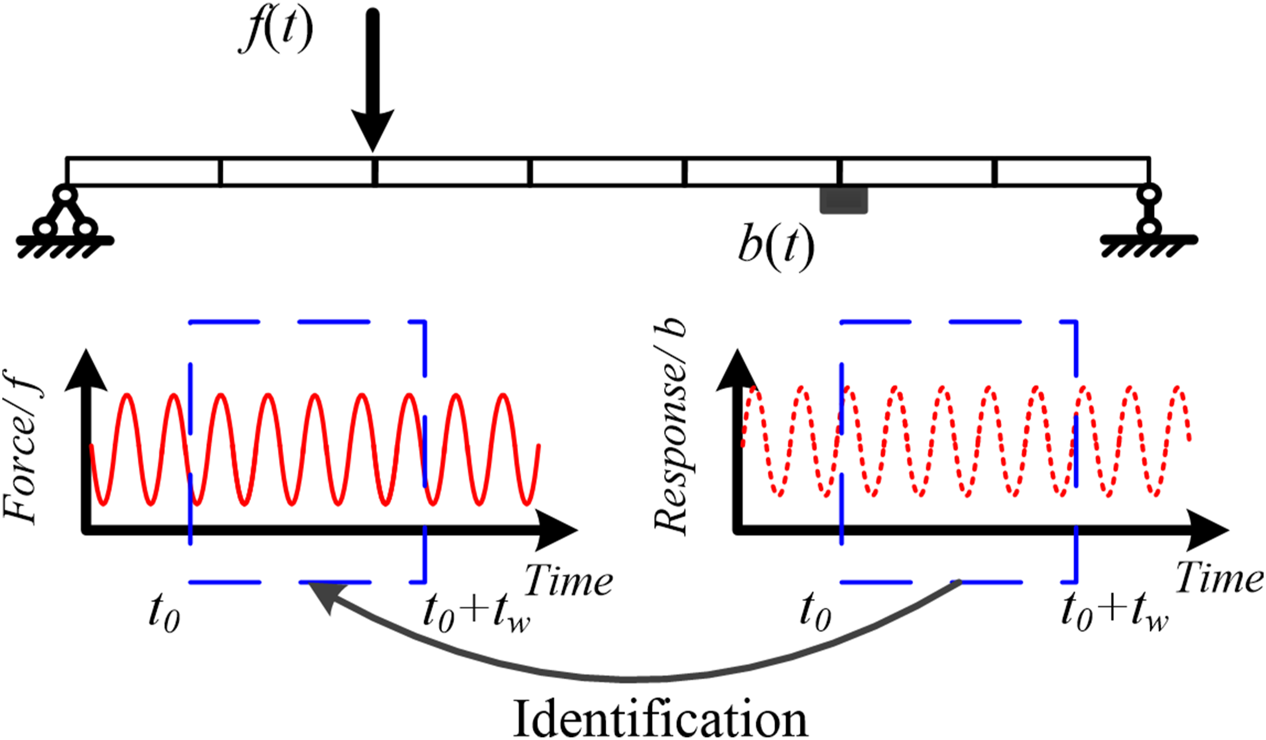 $(t_{0}, t_{0} + t_{w}]$ by using structural responses measured from the same time range. Without loss of generality, the time instant t₀ can be set as 0 s. The acting position of the force is assumed to be known. Hence, the dynamic force can be simplified to a function of time, and it can be expressed in a discrete form such as $f = {[f (Δ t), f (2 Δ t), \dots, f (k Δ t)]}^{T} (f \in R^{k * 1})$ . Herein, Δt is a discrete time interval, and we have $k Δ t = t_{w}$ . A dictionary is introduced for expanding the force as in (Qiao et al., 2016)

f = [d_{1}, d_{2}, \dots, d_{n}] [\begin{matrix} α_{1} \\ α_{2} \\ ⋮ \\ α_{n} \end{matrix}] = Dα

(1)

where

D \in R^{k * n}

means a force dictionary, and it is defined as

D = [d_{1}, d_{2}, \dots, d_{n}]

d_{i} \in R^{k * 1}

is the i-th atom, and

α \in R^{n * 1}

is applied for storing the coefficients. To derive a definition of the concomitant mapping matrix, we extend the length of the analysis time as double the length of t_w. Correspondingly, the force can be extended as

\bar{f} = {[f (Δt), f (2 Δt), \dots, f (kΔt), 0,0, \dots, 0]}^{T} 1,2, \dots, k

(2)

where

\bar{f} \in R^{2 k * 1}

is an extended force. From equation (2), it is found that the first half of

\bar{f}

means the real dynamic force that is considered in this section. Based on this idea, equation (1) also can be extended as

\bar{f} = [\begin{matrix} d_{1} & d_{2} & \dots & d_{n} \\ 0 & 0 & \dots & 0 \end{matrix}] α = \bar{D} α

(3)

where

\bar{D} \in R^{2 k * n}

is an extended dictionary. Assuming that the structure is subjected to the extended force and the length of the analysis time range is considered as 2t_w, structural responses which occurred at one of the measuring points can be expressed as

\bar{b} = [{\bar{h}}_{1}, {\bar{h}}_{2}, \dots, {\bar{h}}_{n}] α = \bar{H} α

(4)

where

\bar{b} \in R^{2 k * 1}

represents the extended structural responses, and it is defined as

\bar{b} = {[b (Δ t), b (2 Δ t), \dots, b (kΔ t), b ((k+ 1) Δ t), b ((k+ 2) Δ t), \dots, b (2 kΔ t)]}^{T}

\bar{H} \in R^{2 k * n}

is a system mapping matrix, in which

{\bar{h}}_{i} \in R^{2 k * 1}

means the i-th response component that is induced by the i-th atom of the dictionary

\bar{D}

Similar to the definition of the extended force, the system mapping matrix shown in equation (4) can be rewritten as

\bar{H} = [\begin{matrix} H_{f} \\ H_{Y} \end{matrix}]

(5)

where

H_{f} \in R^{k * n}

has the same size as

H_{Y} \in R^{k * n}

. In this study, these two matrices are defined as:

H_f, a force-induced mapping matrix.

H_Y, a concomitant mapping matrix corresponding to the force-induced mapping matrix H_f.

2.2. Linear relationship between excitation sources and structural responses

Now, let us come back to the original topic that means the problem of force identification is considered from 0 s to t_w. The structural initial conditions, that is, vibration state at time instant 0 s, are considered. In view of this, the structural responses are contributed from both the force and the initial conditions. According to the physical meaning of H_f and equation (1), the force-induced responses can be expressed as

b_{f} = H_{f} α

(6)

where

b_{f} = {[b (Δ t), b (2 Δ t), \dots, b (kΔ t)]}^{T} (b_{f} \in R^{k * 1})

represent the force-induced responses. Let us assume that the initial condition–caused responses can be expressed as a linear combination of columns of H_Y. This assumption is based on a fact that all columns of H_Y belong to the responses caused by free vibration. However, it should note that the space spanned by the columns of H_Y is not necessarily complete for expressing the responses induced by the real initial conditions. It is because that a space used for completely expressing all the possible responses caused by the real initial conditions should be infinite-dimensional because the real structure belongs to an infinite-degree-of-freedom system. According to the above assumption, the initial condition–caused responses can be expressed as

b_{Y} = H_{Y} Y

(7)

where

b_{Y} = {[b (Δ t), b (2 Δ t), \dots, b (kΔ t)]}^{T} (b_{Y} \in R^{k * 1})

represent the initial condition–caused responses.

Y \in R^{n * 1}

is applied for storing the coefficients corresponding to H_Y.

According to equations (6) and (7), the structural responses $b \in R^{k * 1}$ caused by both the dynamic force and the initial conditions can be expressed as

b = b_{f} + b_{Y} = [H_{f}, H_{Y}] [\begin{array}{l} α \\ Y \end{array}]

(8)

Herein, it should be noted that the structural response vector b is not an instance of the extended structural response vector $\bar{b}$ . In an ideal case, that is, when measurement noises are not considered, the structural response vector b represents the measured structural responses. However, the extended structural response vector $\bar{b}$ is only applied for theoretical analysis in this study. The above equation shows a linear relationship between one force and one measuring point. For a multi-input and multi-output system, equation (8) can be further expanded as a weighted equation as in (Pan et al., 2018; Sun and Büyüköztürk, 2015)

[\begin{matrix} \frac{b_{1}}{{‖ b_{1} ‖}_{2}} \\ \frac{b_{2}}{{‖ b_{2} ‖}_{2}} \\ ⋮ \\ \frac{b_{n_{s}}}{{‖ b_{n_{s}} ‖}_{2}} \end{matrix}] = [\begin{matrix} \frac{H_{f, 11}}{{‖ b_{1} ‖}_{2}} & \frac{H_{f, 12}}{{‖ b_{1} ‖}_{2}} & \dots & \frac{H_{f, 1 n_{f}}}{{‖ b_{1} ‖}_{2}} & \frac{H_{Y, 11}}{{‖ b_{1} ‖}_{2}} & \frac{H_{Y, 12}}{{‖ b_{1} ‖}_{2}} & \dots & \frac{H_{Y, 1 n_{f}}}{{‖ b_{1} ‖}_{2}} \\ \frac{H_{f, 21}}{{‖ b_{2} ‖}_{2}} & \frac{H_{f, 22}}{{‖ b_{2} ‖}_{2}} & \dots & \frac{H_{f, 2 n_{f}}}{{‖ b_{2} ‖}_{2}} & \frac{H_{Y, 21}}{{‖ b_{2} ‖}_{2}} & \frac{H_{Y, 22}}{{‖ b_{2} ‖}_{2}} & \dots & \frac{H_{Y, 2 n_{f}}}{{‖ b_{2} ‖}_{2}} \\ ⋮ & ⋮ & ⋱ & ⋮ & ⋮ & ⋮ & ⋱ & ⋮ \\ \frac{H_{f, n_{s} 1}}{{‖ b_{n_{s}} ‖}_{2}} & \frac{H_{f, n_{s} 2}}{{‖ b_{n_{s}} ‖}_{2}} & \dots & \frac{H_{f, n_{s} n_{f}}}{{‖ b_{n_{s}} ‖}_{2}} & \frac{H_{Y, n_{s} 1}}{{‖ b_{n_{s}} ‖}_{2}} & \frac{H_{Y, n_{s} 2}}{{‖ b_{n_{s}} ‖}_{2}} & \dots & \frac{H_{Y, n_{s} n_{f}}}{{‖ b_{n_{s}} ‖}_{2}} \end{matrix}] [\begin{matrix} α_{1} \\ α_{2} \\ ⋮ \\ α_{n_{f}} \\ Y_{1} \\ Y_{2} \\ ⋮ \\ Y_{n_{f}} \end{matrix}]

(9)

where

b_{i} \in R^{k * 1}

are the structural responses measured from the i-th sensor.

H_{f, i j} \in R^{k * n}

is a force-induced mapping matrix corresponding to the j-th force and the i-th sensor.

H_{Y, i j} \in R^{k * n}

is an concomitant mapping matrix corresponding to the force-induced mapping matrix H_f,ij.

α_{i} \in R^{n * 1}

contains the information of the i-th force.

Y_{i} \in R^{n * 1}

is used for storing the coefficients corresponding to the concomitant mapping matrix H_Y,ij. From equation (9), it can find that the initial conditions are expressed by using the concomitant mapping matrices that are first defined in this study.

Going back to the beginning, the reason why we use the concomitant mapping matrices for expressing the initial conditions is that this strategy can ensure that each basic component of the excitation sources has the same signal energy. For the component of force, this point of view is easy to be understood because the 2-norm value of each atom in the force dictionary is the same. For the component of initial conditions, the concept of energy input to the structure actually has been transformed to the corresponding atom in the force dictionary when the concomitant mapping matrix is applied. To make it intuitive, Figure 2 is introduced for explaining a physical process behind the concept of concomitant mapping matrix. Herein, the analysis time range is assumed as $(- t_{w}, t_{w}]$ . Assuming that the structure is static at the time instant $- t_{w}$ and the loading position analyzed in time range $(- t_{w}, 0]$ is the same as the ones considered in time range $(0, t_{w}]$ , then similar to the expression of equation (1), a same dictionary D can be applied for expressing the force happening in time range $(- t_{w}, 0]$ . In this way, it is found that the structural responses calculated from each atom of the force dictionary D corresponding to time range $(- t_{w}, 0]$ are similar to the ones defined in the concomitant mapping matrix.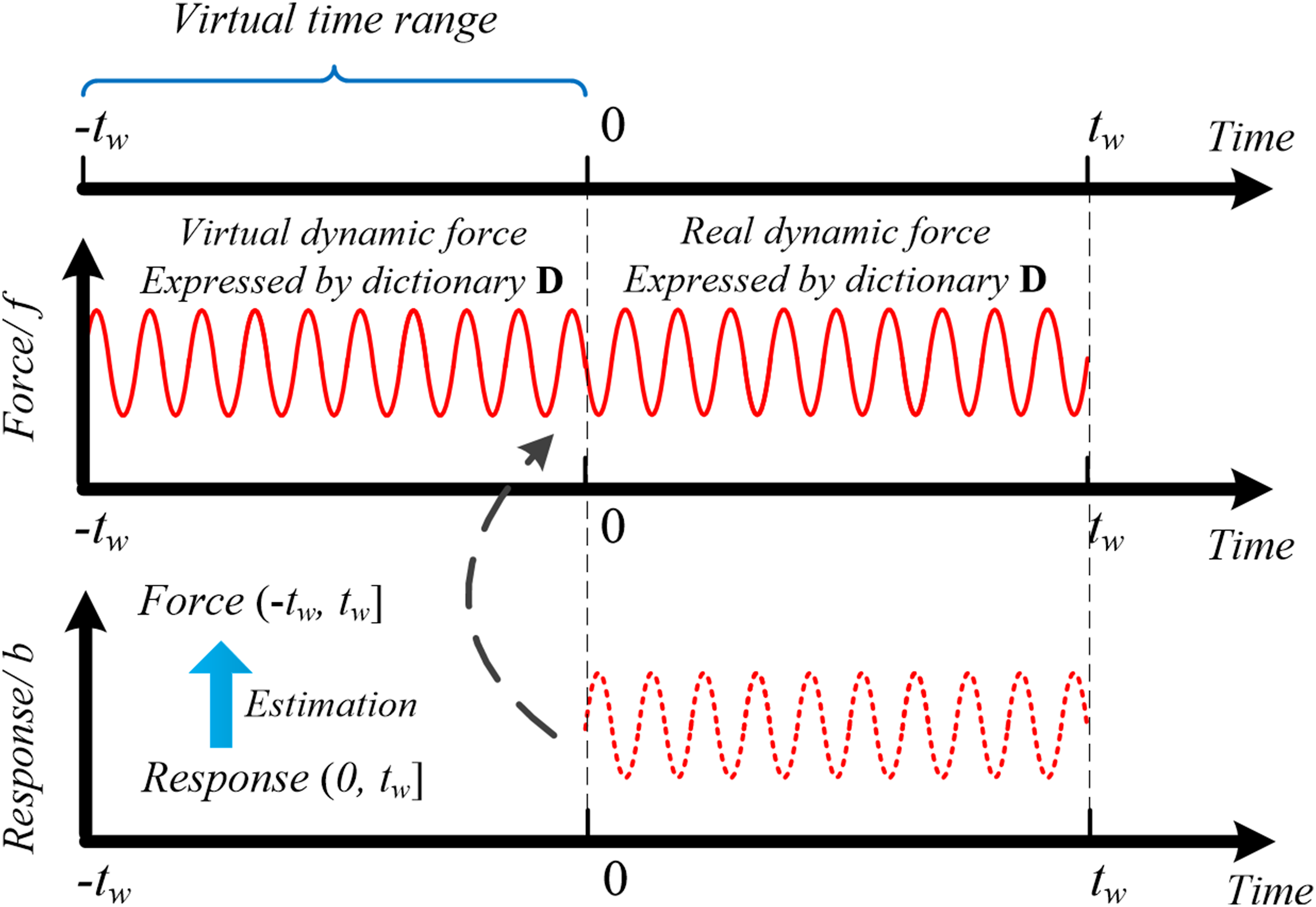 In this sense, when an inverse analysis is taken for identifying the forces by using equation (9), this identified process estimates the forces happening in time range $(- t_{w}, t_{w}]$ by using the structural responses measured from 0 s to t_w. In this virtual identification process, it is found that the signal energy calculated from each force component is equal to each other.

2.3. Force identification based on sparse regularization

Equation (9) can be rewritten as $b = Aβ$ , where b contains the structural responses, A is a system mapping matrix, and β means the excitation sources. To ensure that the identified results are robust enough, the l₁-norm regularization will be recommended in this article (Qiao et al., 2016). Hence, an optimization problem can be established as

β_{identified} = \underset{β}{\arg \min} {{‖ Aβ - b ‖}_{2}^{2} + λ {‖ β ‖}_{1}}

(10)

where β_identified are the identified sources. λ ≥ 0 is a regularization parameter. Equation (10) can be solved by using the fast iterative shrinkage–thresholding algorithm (FISTA) (Beck and Teboulle, 2009).

By solving equation (10), the coefficient vector of excitation sources can be estimated indirectly. Then, we can extract the coefficients corresponding to the forces from β_identified. Finally, the time histories of the forces can be reconstructed according to equation (1). To sum up, the main steps of the proposed method can be listed as:

Step 1. Establish a finite element model (FEM) of the considered structure. Extract the measured structural responses corresponding to a time range $(0, t_{w}]$ .

Step 2. Select a proper dictionary for the expression of dynamic forces.

Step 3. Calculate the system mapping matrices, including the force-induced mapping matrices H_f and their concomitant mapping matrices H_Y. This is the main innovation point of the proposed method.

Step 4. Formulate an identified optimization problem by using the l₁-norm regularization, as shown in equation (10).

Step 5. Solve the optimization problem by using the algorithm named FISTA. Then, calculate the time histories of the dynamic forces according to equation (1).

3. Numerical verifications

3.1. Force identification on plane frame structure

As shown in Figure 3, a frame structure subjected to a lateral force is considered. This structure is referenced from an article published by Li and Hao (2016). Each element has a length of 2 m, 2 nodes, and 6 degrees of freedom (DOF). The cross-section area is 0.32 m². The moment of inertia is 0.017 m⁴. The material parameters are simulated as Young’s modulus E = 35 GPa and density ρ = 2500 kg. The time histories of the force are simulated as a process of band-limited white noise. Its signal energy is mainly located in a frequency range [2 Hz, 50 Hz]. Two sensors installed at nodes 30 and 38 are used for collecting the lateral acceleration responses. Herein, it is hoped that the two measuring sensors are relatively and evenly distributed. Furthermore, the number of sensors is assumed to be more than the number of external force. It is because that both the unknown force and the unknown initial conditions are considered in our identified task. The mode superposition method is applied for response calculation. The first 10 modes with damping ratio 0.012 are considered. The time interval Δt is equal to 0.001 s. The measured noises are simulated as (Pan et al., 2018)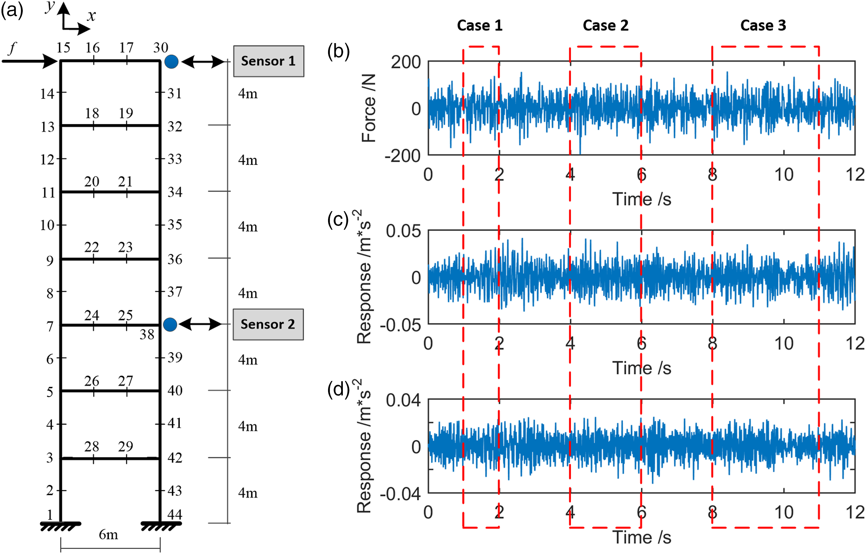

b_{noise} = b + lev \times \frac{1}{k} \sum_{i = 1}^{k} | b (i) | \times rand

(11)

where b_noise and b are the responses for noise and noiseless, respectively. k is the element number in the vector b. lev is the noise level. rand is a standard normal distribution vector. The simulated force and the structural responses with 10% noise level are plotted in Figure 3.

3.1.1. Verification of proposed method

The acceleration responses measured from 1 s to 2 s are extracted for force identification. The construction of force dictionary is a key problem. For a specific case, signal features of the force should be carefully taken into consideration (Qiao et al., 2016). In this case, the force dictionary is built via some basic trigonometric functions as in (Pan and Yu, 2019)

d_{i} (t) = {\begin{matrix} 1 & i = 1 \\ \sin (\frac{i π (t - t_{0})}{T}) & i \in even \\ \cos (\frac{(i - 1) π (t - t_{0})}{T}) & i \in odd \end{matrix} i = 1,2, \dots, n_{t}

(12)

where T and t₀ are the time length and the start time of the identified task, respectively. n_t is the number of basic functions, and it can be calculated as

n_{t} = ⌊ 2 T f_{r} + 0.5 ⌋

(13)

where f_r means the interested highest frequency of the force, and it will be manually selected as f_r = 100 Hz in this case.

⌊ ⌋

is an operator for rounding the value to the nearest integer toward minus infinity. Each basic function will be sampled and normalized

({‖ d_{i} ‖}_{2} = 1)

for formulating the force dictionary D.

The force-induced mapping matrix H_f and its corresponding concomitant mapping matrix H_Y are calculated via five main steps, which can be orderly listed as follows:

The i-th atom d_i (i = 1 for the first iteration) of the force dictionary D is taken as the input source of the frame structure.

As a forward problem, the structural responses induced by the considered input source d_i are calculated. Herein, the forward analysis time length is set as 2 s, which is double the time length corresponding to the original problem of force identification.

The first half part of the calculated structural responses, that is, the calculated structural responses extracted from 0 s to 1 s, is orderly stored in the i-th column of H_f. The matrix H_f contains 2000 rows because the number of sensors simulated in this case is 2.

The latter half part of the calculated structural responses, that is, the calculated structural responses extracted from 1 s to 2 s, is orderly stored in the i-th column of H_Y. The matrix H_Y contains 2000 rows because the number of sensors simulated in this case is 2.

Let i = i + 1, and then do the above steps again until the value of i is equal to 201.

In this case, the rank values of H_f and H_Y are $rank (H_{f}) = 200 and rank (H_{Y}) = 20$ , respectively. The numbers of columns contained in H_f or H_Y are equal to 200. Hence, H_f is a column full rank matrix. This is because that the basic functions defined in equation (12) are linearly independent. Contrarily, H_Y is a low-rank matrix. It is because only the first 10 modes of the frame structure are considered so that the number of independent components corresponding to the initial conditions should not be bigger than 20 in theory.

The FISTA with an initial value 0 and 5000 iteration steps is applied for the solution. The regularization parameter listed in Table 1 is selected by using Bayesian information criteria (BIC) (Pan and Yu, 2019; Pan et al., 2018). Relative percentage error (RPE) is introduced for evaluating the identified accuracy as

RPE = \frac{{‖ f_{identified} - f_{real} ‖}_{1}}{{‖ f_{real} ‖}_{1}} \times 100 %

(14)

where f_identified and f_real are the identified force and the actual force, respectively. The RPE value of the considered case is also listed in Table 1.

Table 1.

Relative percentage error and some additional information in case 1.

Regularization parameter	2.1779 × 10⁻⁶
Number of elements in vector β_identified	400
Number of nonzero elements in vector β_identified	129
Relative percentage error	13.28%

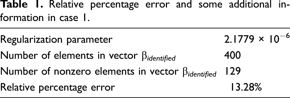
Figure 4(a) plots the identified coefficient β_identified. From Figure 4(a) and Table 1, it can be seen that there are 271 (400 − 129 = 271) zero elements in the identified vector β_identified so that the identified vector β_identified is sparse. This is a natural result because of the application of sparse regularization. In addition, Figure 4(a) shows that Y-values of the latter half part of elements corresponding to the force are zero or close to zero. The reason is that the energy of the simulated force is lower than or equal to 50 Hz, which is equal to one-half of the interested highest frequency. Furthermore, Figure 4(a) shows that nonzero initial conditions are included. It is reasonable because the frame structure is under the action of load before the start time considered in this case. Comparisons on the actual responses and the reconstructed responses are shown in Figure 4(b)–(e). These subfigures show that the reconstructed responses are close to the actual ones. Herein, the initial conditions represent the structural vibration state at the start time of this identified task. These results mean that the mixed responses, that is, force-induced responses, initial condition–caused responses and noises, can be effectively separated by using the proposed method.

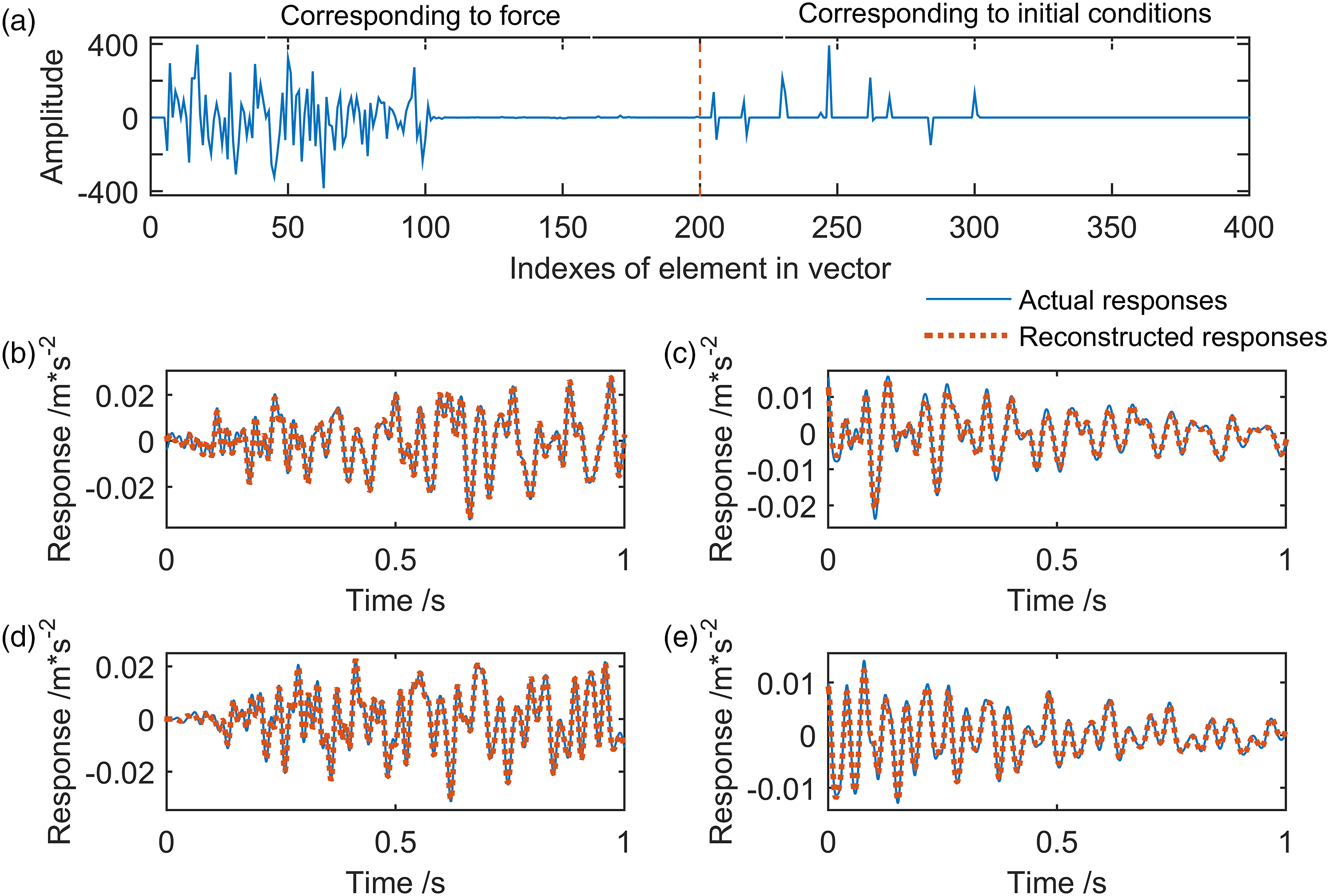
Figure 5 shows the comparisons on time histories of the actual force and the identified force. The identified accuracy RPE also has been calculated and listed in Table 1. From Figure 5 and Table 1, it can be seen that the identified force matches well with the actual ones. This result actually means that the proposed method is feasible and effective for the solution of force identification in the considered case.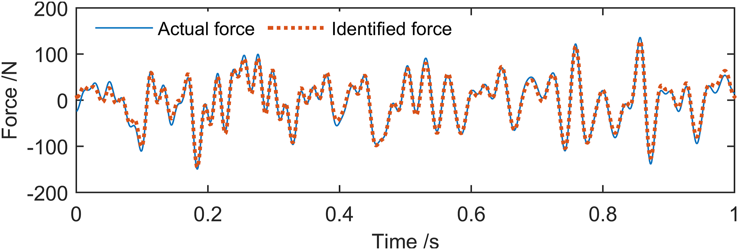

3.1.2. Influences of measurement noises

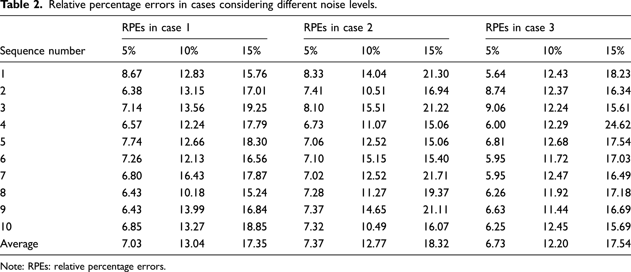
The force happening in three time ranges such as (1 s, 2 s], (4 s, 6 s], and (8 s, 11 s] will be identified in case 1, case 2, and case 3, respectively. Three noise levels such as 5%, 10%, and 15% are considered. Other calculation parameters are selected similar to the ones considered in the previous section. Each case considering one noise level is calculated 10 times independently. A random seed applied for simulating the measured noises is determined by using an operating system clock in real time. Table 2 lists all the RPE values that are calculated from all the independent calculations.

Table 2.

Relative percentage errors in cases considering different noise levels.

Sequence number	RPEs in case 1			RPEs in case 2			RPEs in case 3
Sequence number	5%	10%	15%	5%	10%	15%	5%	10%	15%
1	8.67	12.83	15.76	8.33	14.04	21.30	5.64	12.43	18.23
2	6.38	13.15	17.01	7.41	10.51	16.94	8.74	12.37	16.34
3	7.14	13.56	19.25	8.10	15.51	21.22	9.06	12.24	15.61
4	6.57	12.24	17.79	6.73	11.07	15.06	6.00	12.29	24.62
5	7.74	12.66	18.30	7.06	12.52	15.06	6.81	12.68	17.54
6	7.26	12.13	16.56	7.10	15.15	15.40	5.95	11.72	17.03
7	6.80	16.43	17.87	7.02	12.52	21.71	5.95	12.47	16.49
8	6.43	10.18	15.24	7.28	11.27	19.37	6.26	11.92	17.18
9	6.43	13.99	16.84	7.37	14.65	21.11	6.63	11.44	16.69
10	6.85	13.27	18.85	7.32	10.49	16.07	6.25	12.45	15.69
Average	7.03	13.04	17.35	7.37	12.77	18.32	6.73	12.20	17.54

Note: RPEs: relative percentage errors.

From Table 2, it can be seen that the identified accuracies obtained from different calculations are not equal to each other, even though the same noise level is considered. It is reasonable because the measured noises are simulated as a random process. Furthermore, three average RPEs corresponding to case 1 clearly show that the identified accuracy decreases with increasing noise level in case 1. The same phenomenon can be seen from case 2 and case 3. This phenomenon means that measurement noises can bring a negative effect to the identified results in the considered cases. To make it intuitive, Figure 6 shows the forces calculated from case 2 considering different noise levels. It clearly shows that the identified error mainly comes from the shrink of amplitude of signal features. The reason may be because of the application of l₁-norm regularization. Generally, amplitudes of force features will be shrunk slightly when l₁-norm regularization is applied for shrinking the noises. Hence, a large noise level can naturally lead to a larger reduction of the amplitudes of force features.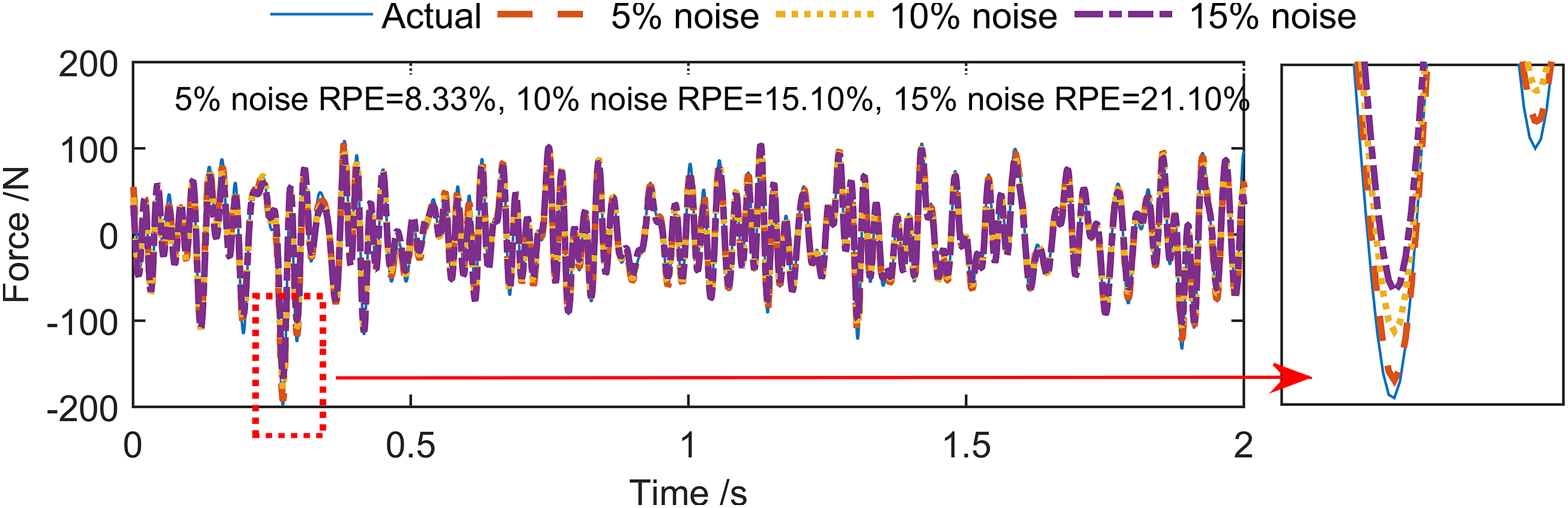

In spite of the RPEs listed in Table 2, Figure 6 clearly shows that the proposed method can provide an acceptable identification result even though the noise level is simulated as 15%. In addition, Table 2 also shows that there is no significant difference among the RPEs calculated from case 1, case 2, and case 3. This characteristic represents that the identified result is not sensitivity to the length of the identified task considered in this section. This advantage may be contributed from the consideration of unknown initial conditions.

3.1.3. Comparisons on different methods

Case 1 shown in Figure 3 is taken for discussion. Measurement noises with 10% level are considered. The force will be identified by using the proposed method and an existing method proposed based on truncated response sparse decomposition (TRSD) (Pan and Yu, 2019), respectively. The l₁-norm regularization is applied for response decomposition when the TRSD-based method is applied. The regularization parameter is selected according to the BIC. Two key values such as acceptable levels for scaling factor and response energy are selected as κ_σ = κ_χ = 0.01 (Pan and Yu, 2019).

The relationship between excitation sources and responses is expressed as an equation such as $b = Aβ$ , where b contains the structural responses, A is the system matrix, and β means the excitation sources. It can be found that the size of system matrix A applied for the TRSD-based method is 2000 × 220, including 200 columns for expanding the dynamic force and 20 columns for expanding the initial conditions. However, the size of system matrix A corresponding to the proposed method is 2000 × 400. This size is actually bigger than the one corresponding to the TRSD-based method. Hence, relatively speaking, more computing resources are usually needed when the proposed method is applied. For example, in this study, the CPU times spent for solving case 1 via using the proposed method and the TRSD-based method are 13.2846 s and 12.1649 s, respectively.

Figure 7 shows the 2-norm value of each column of the system matrix A. From Figure 7, it can be been that two curves are equal to each other for a segment representing the force component–induced responses. It is mainly because that the force dictionaries applied for the two methods are the same. Figure 7 also shows that the 2-norm values of columns corresponding to t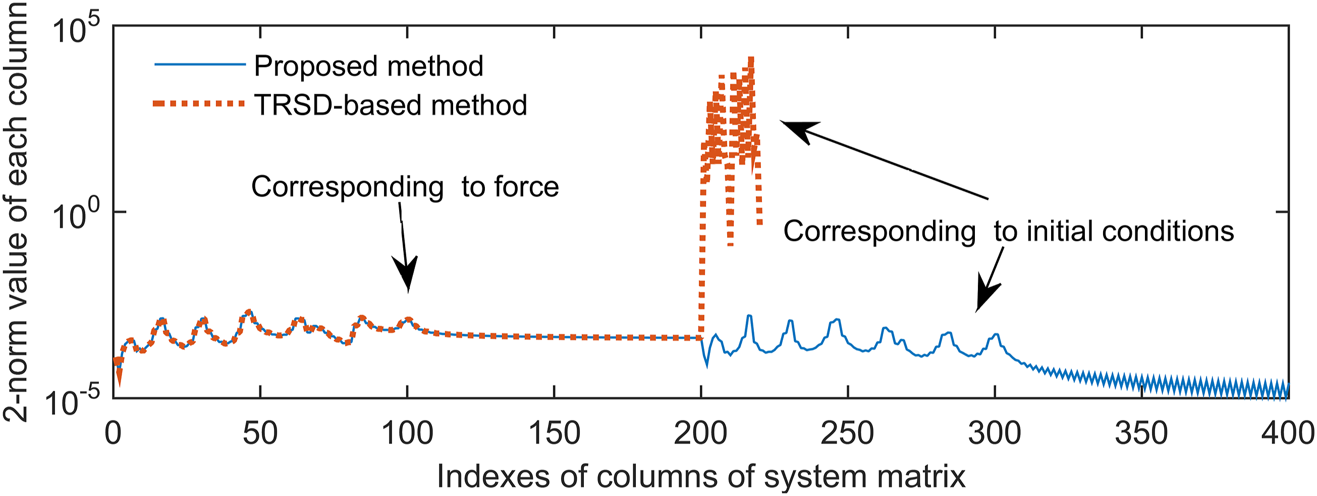he initial conditions are much bigger than ones corresponding to the force in the TRSD-based case. However, the above phenomenon cannot be seen from the curve corresponding to the proposed method. Instead, the curve corresponding to the proposed method is much smoother than the other curve. There is no obvious sharp break between the Y-values corresponding to the force and the ones corresponding to the initial conditions. This result is a main advantage of the proposed concomitant mapping matrix.

Figure 8 shows the identified forces. It clearly shows that both the proposed method and the TRSD-based method can be applied for identifying the force in the considered case. Overall, comparing with the TRSD-based method, the proposed method can effectively reduce the possible large numerical difference between the response components corresponding to force and initial conditions. Hence, the force can be identified by using a one-step strategy proposed in this study.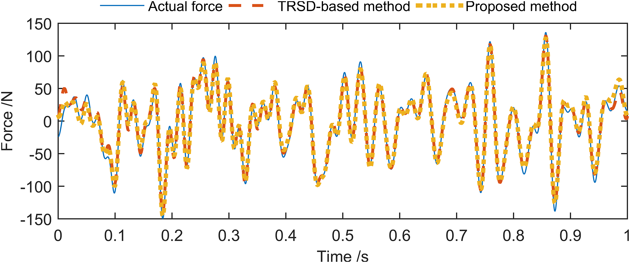

3.2. Moving force identification on continuous bridge

An interchange ramp bridge is taken for further verifying the proposed method. The continuous bridge has 90 m long with three equal spans, as shown in Figure 9. Superstructure of the considered bridge is a concrete continuous single-cell box girder with a constant section. A simplified two-dimensional FEM is established. The total bridge is equally divided into 90 elements. Each element has 2 nodes and 4 DOF. Hinged supports are simulated. The bending stiffness and density of unit length are selected as EI = 6.3135 × 10¹⁰ N m² and ρA = 10,060 kg m⁻¹, respectively. The first five natural frequencies of this continuous bridge are 4.37 Hz, 5.60 Hz, 8.18 Hz, 17.49 Hz, and 19.93 Hz, respectively. Two forces move through the bridge with a constant speed 7.5 m/s. The distance between two forces is simulated as 4.2 m. Three sensors are installed at L1 section, L2 section, and L3 section for measuring the bending moment responses. The model superposition method with the first 20 orders is used for simulating the structural responses. Herein, the reason why 20 modes are considered is relatively simple. In fact, some test calculations with different orders have been done before the above selection, and we find that selection of 20 modes is considerable for both the accuracy and efficiency of calculation. The damping ratio for each order is selected as ξ_i = 2%. The sampling frequency is set as 1000 Hz. The white noises are calculated via using equation (11). The time histories of each moving force are simulated as the sum of an axle weight and a random load component (Sun et al., 2015). Herein, the axle weights are simulated as 40 kN and 60 kN for the front force and the rear force, respectively. The random component is simulated as a band limited signal, and its signal energy is mainly located in a frequency range [2 Hz, 50 Hz]. Both the time histories and the bending moment responses are plotted in Figure 10.

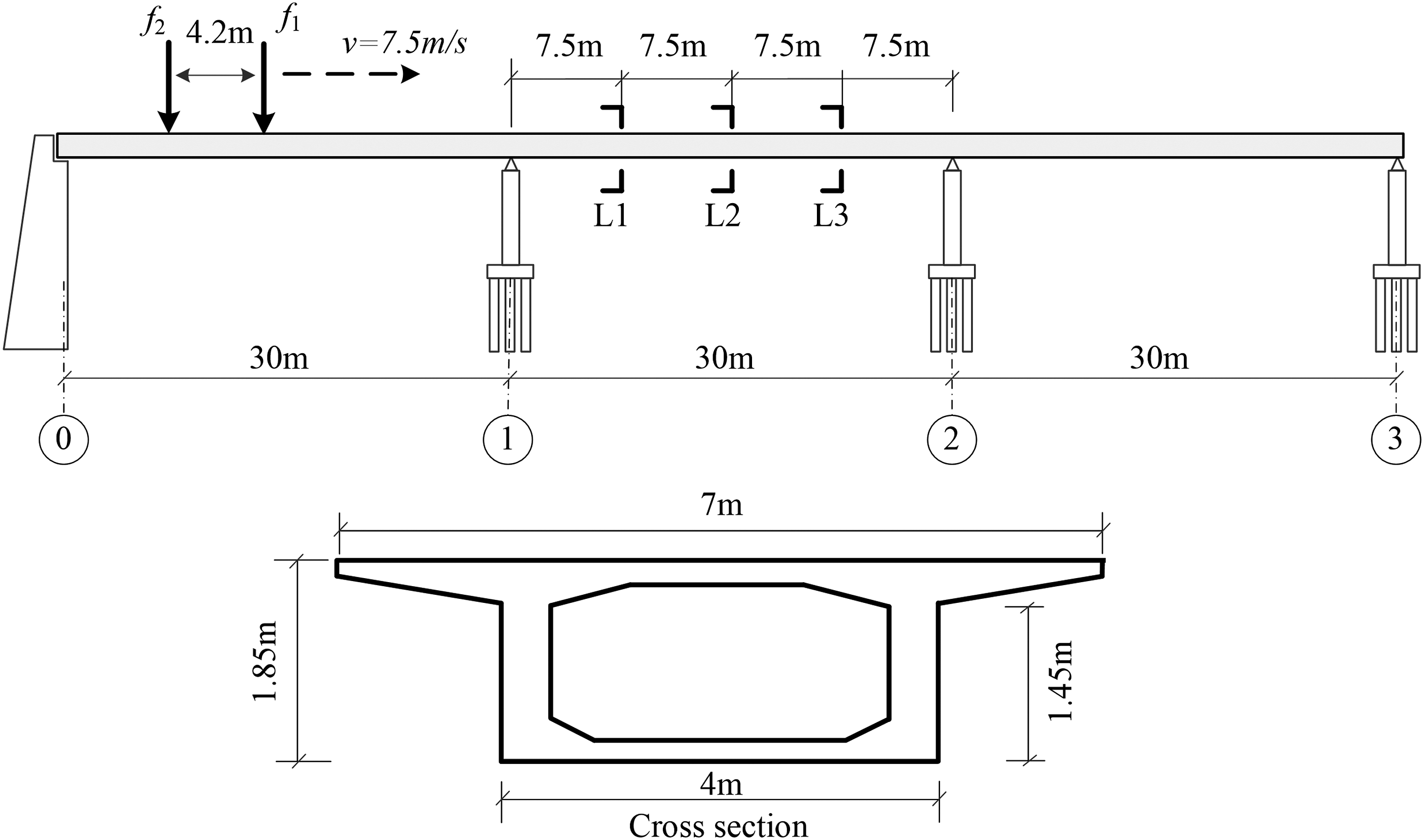
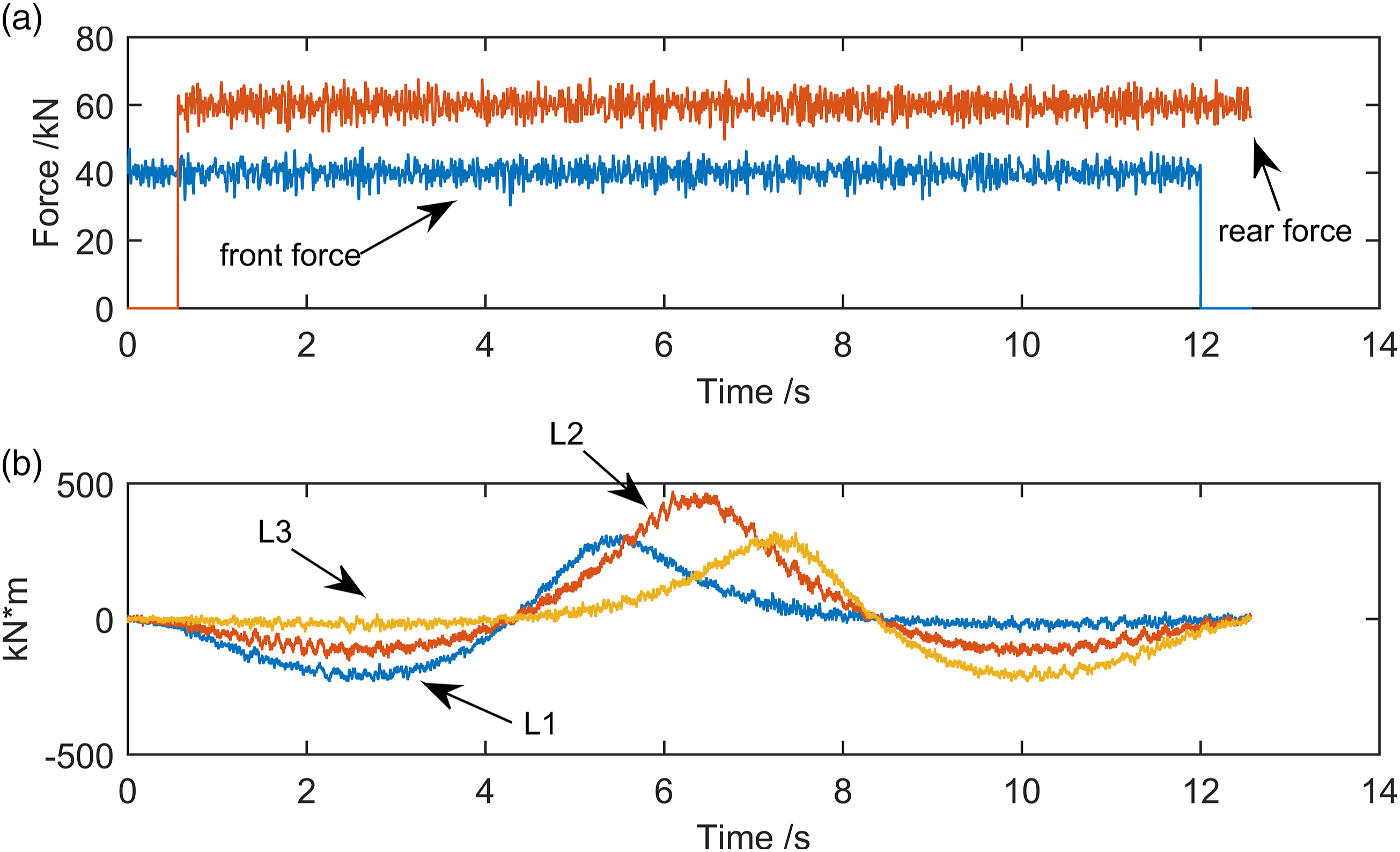
The structural responses measured from 4.56 s to 8.00 s are extracted for calculation. This time segment corresponds to a situation that two moving forces totally move on the middle span of the bridge. The force dictionary is defined as the one that has been done in Section 3.1. The interested highest frequency of moving forces is selected as f_r = 100 Hz. Other parameters applied for solving the l₁-norm regularization–based equation are selected similar to the ones done in Section 3.1.

The estimated coefficient β_identified and the identified moving forces are plotted in Figure 11. Herein, the number of the nonzero elements in β_identified is equal to 404, which is smaller than 2748, that is, the element number of the vector β_identified. From Figure 11(a), it can be seen that both the force-induced responses and the initial condition–caused responses are contained in the measured responses. This is mainly because only the middle span of the bridge is taken as a test section in this study. However, the forces are simulated to move through the first span before they enter the test section. Furthermore, Figure 11(b) and (c) clearly show that the trend lines of the identified moving forces are close to the real axle weights. It means that the proposed method has a good ability to estimate the axle weights in the considered case. To make it more clear, two estimated axle weights are calculated and listed in Table 3. Herein, the estimated axle weight is calculated by using a mean value of the identified force.

Table 3.

Estimated axle weights and relative percentage error of identified moving forces.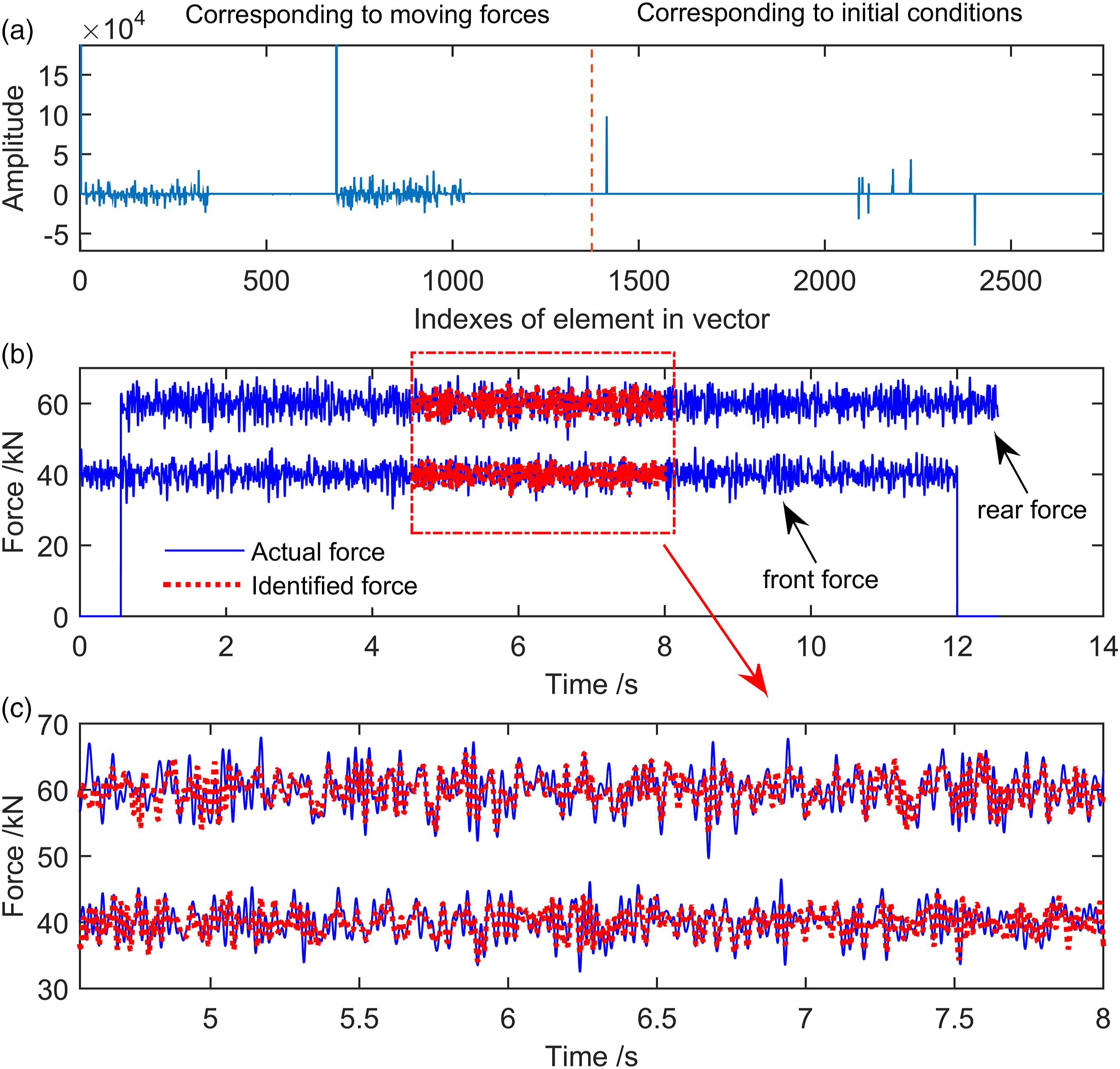

Force	Axle weight			Relative percentage error (%)
Force	Estimated (w_e) (kN)	Real (w_f) (kN)	Relative error (\|w_e − w_f\|/w_f) (%)	Relative percentage error (%)
Front	39.9496	40	0.13	2.92
Rear	59.9799	60	0.03	2.24

In addition, the time-varying components of the identified forces can match the actual ones to some extent, as shown in Figure 11(c). However, the identified accuracy of these parts is intuitively lower than the identified accuracy of the axle weights. The reason behind this phenomenon is that most proportions of bending moment responses, which are applied for force identification, are mainly caused by the time-invariant components of moving forces, that is, axle weights (Pan et al., 2018). Hence, the reconstruction of time-varying force components is relatively easier to be influenced by the measured noises. In spite of the above disadvantage, the identified moving forces shown in Figure 11 and RPE values listed in Table 3 actually show that our proposed method is feasible and effective for identifying the moving forces in the considered cases.

4. Conclusions

A novel sparse regularization–based method is proposed for force identification considering unknown initial conditions. The concept of concomitant mapping matrix is first introduced for expressing the unknown initial conditions. Herein, the concomitant mapping matrix is formulated by using free vibrating responses, which corresponds to the structural responses happening after the structure is subjected to each atom of a force dictionary. Then, combining with the sparse regularization, the problem of force identification can be converted into an optimization problem, which can be solved by using a one-step strategy.

Numerical simulations are carried out for assessing the feasibility and effectiveness of the proposed method. The illustrated results show that the proposed method has a good ability for reconstructing the simulated force and the moving forces in the considered cases, even though the structural initial conditions are not equal to zero and unknown to us. The illustrated results also show a good robustness of the proposed method to some extent. Comparing with the existing two-step method, the proposed method actually can be regarded as a one-step strategy.

Footnotes

Declaration of conflicting interests

The author(s) declared no potential conflicts of interest with respect to the research, authorship, and/or publication of this article.

Funding

The author(s) disclosed receipt of the following financial support for the research, authorship, and/or publication of this article: This work was supported by National Natural Science Foundation of China under Grant 51908149.

ORCID iDs

Xijun Ye

Chudong Pan

References

Aucejo

De Smet

(2018) A space-frequency multiplicative regularization for force reconstruction problems. Mechanical Systems and Signal Processing 104: 1–18.

Beck

Teboulle

(2009) A fast iterative shrinkage-thresholding algorithm for linear inverse problems. SIAM Journal on Imaging Sciences 2(1): 183–202.

Chen

Qin

Zhao

, et al. (2019) Toward efficacy of piecewise polynomial truncated singular value decomposition algorithm in moving force identification. Advances in Structural Engineering 22(12): 2687–2698.

Guo

Ding

Wang

, et al. (2018) A dynamic load estimation method for nonlinear structures with unscented Kalman filter. Mechanical Systems and Signal Processing 101: 254–273.

Wang

Ren

(2019) Dynamic force identification based on composite trigonometric wavelet shape function. Mechanical Systems and Signal Processing 141: 106493.

Jayalakshmi

Lakshmi

Mohan Rao

(2018) Dynamic force reconstruction techniques from incomplete measurements. Journal of Vibration and Control 24(22): 5321–5344.

Jayalakshmi

Rao

ARM

(2017) Simultaneous identification of damage and input dynamic force on the structure for structural health monitoring. Structural and Multidisciplinary Optimization 55(6): 2211–2238.

Kazemi Amiri

Bucher

(2018) A procedure for continuous estimation of system input force and states. In: 6th European conference on computational mechanics, Glasgow, UK, 11–15 June 2018, pp. 2442–2450. GBR: International Center for Numerical Methods in Engineering (CIMNE).

Law

Chan

THT

Zeng

(1997) Moving force identification: a time domain method. Journal of Sound and Vibration 201(1): 1–22.

10.

Hao

(2016) Substructural interface force identification with limited vibration measurements. Journal of Civil Structural Health Monitoring 6(3): 395–410.

11.

(2018) Time domain force identification based on adaptive ℓ_q regularization. Journal of Vibration and Control 24: 5610–5626.

12.

Zhao

Chen

, et al. (2018) Force identification based on a comprehensive approach combining Taylor formula and acceleration transmissibility. Inverse Problems in Science and Engineering 26(11): 1612–1632.

13.

Liu

Luo

, et al. (2020) Compressed sensing for moving force identification using redundant dictionaries. Mechanical Systems and Signal Processing 138: 106535.

14.

Meggitt

JWR

Moorhouse

Elliott

(2019) A covariance based framework for the propagation of uncertainty through inverse problems with an application to force identification. Mechanical Systems and Signal Processing 124: 275–297.

15.

Pan

(2019) Identification of external forces via truncated response sparse decomposition under unknown initial conditions. Advances in Structural Engineering 22(15): 3161–3175.

16.

Pan

C-D

Liu

H-L

, et al. (2018) Moving force identification based on redundant concatenated dictionary and weighted l₁-norm regularization. Mechanical Systems and Signal Processing 98: 32–49.

17.

Prawin

Rama Mohan Rao

(2018) An online input force time history reconstruction algorithm using dynamic principal component analysis. Mechanical Systems and Signal Processing 99: 516–533.

18.

Qiao

Liu

, et al. (2019) An enhanced sparse regularization method for impact force identification. Mechanical Systems and Signal Processing 126: 341–367.

19.

Qiao

Zhang

Wang

, et al. (2016) Sparse regularization for force identification using dictionaries. Journal of Sound and Vibration 368: 71–86.

20.

Rezayat

Nassiri

De Pauw

, et al. (2016) Identification of dynamic forces using group-sparsity in frequency domain. Mechanical Systems and Signal Processing 70–71: 756–768.

21.

Sanchez

Benaroya

(2014) Review of force reconstruction techniques. Journal of Sound and Vibration 333(14): 2999–3018.

22.

Sanchez

Benaroya

(2017) Asymptotic approximation method of force reconstruction: proof of concept. Mechanical Systems and Signal Processing 92: 39–63.

23.

Sun

Büyüköztürk

(2015) Identification of traffic-induced nodal excitations of truss bridges through heterogeneous data fusion. Smart Materials and Structures 24(7): 075032.

24.

Sun

Feng

Liu

, et al. (2015) Statistical regularization for identification of structural parameters and external loadings using state space models. Computer-Aided Civil and Infrastructure Engineering 30(11): 843–858.

25.

Wang

Zhu

, et al. (2019) Identification of moving train loads on railway bridge based on strain monitoring. Smart Structures and Systems 23: 263–278.

26.

Wang

Liu

Xie

, et al. (2018a) A new regularization method for the dynamic load identification of stochastic structures. Computers & Mathematics with Applications 76(4): 741–759.

27.

Wang

Ren

Liu

(2018b) A novel fractional Tikhonov regularization coupled with an improved super-memory gradient method and application to dynamic force identification problems. Mathematical Problems in Engineering 2018: 1–16.

28.

Chan

THT

(2003) Moving force identification based on the frequency-time domain method. Journal of Sound and Vibration 261(2): 329–349.

29.

Zheng

Wang

(2019) A novel method for force identification based on filter and FEM. Journal of Vibration and Control 25(19–20): 2656–2666.