Time domain force identification based on adaptive ℓ q regularization

Abstract

Traditional time domain force identification methods require prior knowledge about the force profile to apply the appropriate regularization term. Generally speaking, ℓ₁ and ℓ₂ regularization are applied for sparse-type and continuous-type forces respectively. However, prior knowledge about the force type may be unavailable in engineering practice. It is then necessary to incorporate the determination of q (as in ℓ_q regularization) into the identification process. In this paper, we propose two methods to address the problem: the joint and marginal posterior modes of the force history. The identification problem is formulated within the Bayesian framework. The force history, precision parameters, and q are all treated as unknown random parameters, and estimated based on vibration measurements only. The proposed methods are numerically validated on a mass–spring system, an engineering-scale support structure and experimentally validated on a cantilever beam. It is shown that the proposed methods by considering the data-driven determination of q could adapt to the force profile and consistently provide satisfactory results.

Keywords

Force identification time domain inverse problem Bayesian formulation

1. Introduction

The knowledge about external structural excitations is crucial information in structural analysis. It could be used for structural response prediction, health monitoring, and the improvement of future design. Force transducers could be installed to directly measure the desired force histories. However, due to economic and structure integrity considerations, this direct approach is often unfeasible. We instead turn to the indirect/inverse force identification approach. Based on the known structure model and limited measured structural responses, the force history is calculated as the solution to some optimization problem.

Intuitively, the optimization cost function could be the deviation between the measured response and the reconstructed one based on an assumed force history. The identified force history is the solution to the minimization of this object. However, this method usually turns out to be mathematically ill-posed. It means that a little inevitable measurement noise in the measured structural responses would substantially alter the solution to the minimization problem. So, the identified force history by this naive method is hardly believable. The regularization technique is generally considered to stabilize the solution. Regularization adds a penalty term to the naive optimization problem. The amount of regularization is controlled by a positive multiplication parameter. The most widely adopted regularization is undoubtedly Tikhonov regularization, that is, the penalty term is the ℓ₂-norm of the solution. Jacquelin et al. (2003) applied Tikhonov regularization to reconstruct any force on a circular aluminum plate. Two regularization parameter selection criteria are studied: L-curve; and generalized cross validation. Li et al. (2014) introduced wavelet multi-resolution analysis for force history identification. By wavelet decomposition and transform at certain resolutions, the identification of force history is reformulated as the identification of wavelet coefficients. Tikhonov regularization is applied to stabilize the solution. Li and Lu (2017) applied a complex method and Tikhonov regularization for any force localization and identification. The optimization cost function is a function of both unknown force location and history, and is minimized by a two-step approach. Other applications of ℓ₂-norm regularization could be found in Ronasi et al. (2011), Wentzel (2013), Aucejo and De Smet (2016), Li and Lu (2016), and Pan et al. (2017).

ℓ₁-norm regularization has recently become a trending topic for force identification studies. ℓ₁-norm regularization induces the solution of the optimization problem to contain only a few nonzero elements (or so-called sparse). If the force history is sparse (for example an impact), or that it could be sparse-represented in a known transformation basis, ℓ₁-norm regularization generally is more immune to measurement noise than Tikhonov regularization. Qiao et al. (2016b) applied dictionary basis transformation according to the profile of the force, and sparse reconstruction by the separable approximation algorithm to solve the ℓ₁-norm regularization problem. Compared to Tikhonov regularization, more robust solutions were provided from highly noisy measurements. Qiao et al. (2017) also introduced the primal-dual interior point method to solve the large-scale impact identification problem. Experiments including single and consecutive impact force identification proved the robustness and efficiency of the algorithm. Pan et al. (2018) introduced redundant concatenated dictionary transformation and ℓ₁-norm regularization to simultaneously identify both slowly-varying harmonic and impact signals in the bridge–vehicle interaction forces. Other applications of ℓ₁-norm regularization could be found in Samagassi et al. (2015), and Qiao et al. (2016a).

In engineering practice, the external forces on a structure could be arbitrary. The sparsity/continuity property of the force is sometimes a priori unknown, making previous methods inapplicable. In such conditions, a choice between using sparsity-inducing ℓ₁ regularization and continuity-inducing ℓ₂ regularization is demanded. Ideally, this choice, equivalently the value of q in ℓ_q regularization should be automatically and adaptively determined according to the force profile. In this paper, we propose two methods to achieve this, by considering the determination of q based on Bayesian formulation. In the Bayesian framework (Aucejo, 2014; Azam et al., 2015; Feng et al., 2015; Sun and Büyüköztürk, 2015; Aucejo and De Smet, 2016; Faure et al., 2017; Yan et al., 2017), the influence of different parameters, including the unknown force history, the precision parameters (equivalently the regularization parameter) and q, could be easily incorporated. The joint and marginal posterior modes (PMs) of the parameters are proposed for their estimation. The two PMs are respectively solved by conditional maximization (CM) and expectation-maximization (EM) algorithms. Recently, Aucejo and De Smet (2017a) proposed applying the Markov chain Monte Carlo (MCMC) method to sample the posterior distribution of parameters and determine the appropriate q accordingly. However, notice that Aucejo and De Smet (2017a) focus on the spatial reconstruction of vibration sources, while this contribution is more concerned with the adaptive identification of force history. Besides, MCMC sampling is generally time-consuming while in the proposed methods q is determined in a fast-iterative manner.

The rest of the paper is organized as follows. In Section 2, the formulation of the forward problem and Bayesian formulation of the inverse identification problem are given. In Section 3, the force identification methods are proposed and corresponding solution algorithms are given in detail. In Section 4, numerical studies of a mass–spring system and an engineering-scale support structure, and an experimental study of a laboratory-scale cantilever beam are carried out to validate the proposed methods. In all cases, the adaptivity of the proposed methods are tested with various loadings. Their robustness under different levels of both system and measurement noise are also tested. The conclusions are drawn in Section 5.

2. Problem formulation

2.2. Formulation of the forward problem

Suppose a linear elastic structure is excited by a point force at a known location. The structure is spatially discretized with the finite element (FE) method. The system governing equation, in a general form, is

M \overset{··}{y} (t) + C \overset{\cdot}{y} (t) + Ky (t) = L f (t)

(1)

where M, C and

K \in ℝ^{n_{d} \times n_{d}}

are the system mass, damping and stiffness matrices; n_d is the number of physical degree of freedoms (DoFs);

\overset{··}{y} (t), \overset{\cdot}{y} (t)

and

y (t)

are respectively acceleration, velocity and displacement vectors at time t. f(t) is the external force at time t.

L \in ℝ^{n_{d} \times 1}

is the mapping vector for the external force.

The state space (Mobayen, 2015; Mobayen and Javadi, 2016) representation of equation (1) is

\overset{\cdot}{z} (t) = A_{c} z (t) + B_{c} f (t)

(2)

with

\begin{matrix} z (t) = [\begin{matrix} y (t) \\ \overset{\cdot}{y} (t) \end{matrix}], A_{c} = [\begin{matrix} 0 & I \\ - M^{- 1} K & - M^{- 1} C \end{matrix}], \\ B_{c} = [\begin{matrix} 0 \\ M^{- 1} L \end{matrix}] \end{matrix}

(3)

where

A_{c}

is the continuous state space model matrix;

B_{c}

is the input matrix; and I is an identity matrix. When acceleration measurements are available at certain DoFs of a structure, the output is

w (t) = C_{c} z (t) + D_{c} f (t)

(4)

with

C_{c} = [\begin{matrix} 0 & R \end{matrix}] A_{c} and D_{c} = [\begin{matrix} 0 & R \end{matrix}] B_{c}

(5)

Here $C_{c} \in ℝ^{n_{s} \times 2 n_{d}}$ and $D_{c} \in ℝ^{n_{s} \times 1}$ . n_s is the number of accelerometers. $R \in ℝ^{n_{s} \times n_{d}}$ is the response selection matrix; assume zero-order hold for f(t) and convert equation (2) and equation (4) into discrete-time form, we have

z (k + 1) = A_{d} z (k) + B_{d} f (k)

(6)

w (k) = C_{d} z (k) + D_{d} f (k)

(7)

where

z (k), w (k)

and f(k) are discrete vectors and component at time step

t = k Δ t (k = 1, 2, \dots, n_{t})

Δ t

is the sampling interval. n_t is the length of force history vector.

A_{d}, B_{d}, C_{d}

and

D_{d}

are discrete state space model matrices,

\begin{matrix} A_{d} = exp (A_{c} Δ t), B_{d} = A_{c}^{- 1} (A_{d} - I) B_{c}, \\ C_{c} = C_{d}, D_{d} = D_{c} \end{matrix}

(8)

Substitute equation (6) into equation (7) and apply zero initial conditions for both z and F, that is, $z (0) = 0$ and $f (0) = 0$ , we have

W = HF

(9)

with

W = [\begin{matrix} w (1); & w (2); & \dots; & w (n_{t} - 1); & w (n_{t}) \end{matrix}]

(10)

F = [\begin{matrix} f (1) & f (2) & \dots & f (n_{t} - 1) & f (n_{t}) \end{matrix}]^{T}

(11)

\begin{matrix} H = [\begin{matrix} D_{d} & 0 & 0 & \dots & 0 \\ C_{d} B_{d} & D_{d} & 0 & \dots & 0 \\ C_{d} A_{d} B_{d} & C_{d} B_{d} & D_{d} & \dots & 0 \\ : & : & : & : \\ C_{d} A_{d}^{n_{t} - 2} B_{d} & C_{d} A_{d}^{n_{t} - 3} B_{d} & \dots & C_{d} B_{d} & D_{d} \end{matrix}] \end{matrix}

(12)

where

W \in ℝ^{n_{s} n_{t} \times 1}

is the computed acceleration vector;

F \in ℝ^{n_{t} \times 1}

is the assembled force vector; and

H \in ℝ^{n_{s} n_{t} \times n_{t}}

is the lower block system matrix. To simulate measurement noise, a zero-mean Gaussian white noise history

N \in ℝ^{n_{s} n_{t} \times 1}

is added into the computed acceleration history.

X = W + N

(13)

The noise level will be denoted by the noise percentage

‖ N ‖_{2} / ‖ W ‖_{2}

in the following.

2.3. The Bayesian formulation of the identification problem

In this section, the identification problem is formulated within the Bayesian framework. By applying the Bayesian framework, different to-be-determined parameters could be incorporated into the identification problem through Bayesian inference in a similar manner. The quality of different force identification results could naturally be evaluated by corresponding posterior probabilities. The Bayesian framework relies on the Bayes’ rule. Based on contaminated structural response measurements X, the Bayes’ rule describes the probability of unknown variables Y as:

p (Y | X) = \frac{p (X | Y) p (Y)}{p (X)} \propto p (X | Y) p (Y)

(14)

p (X)

could be omitted because it is a constant given a certain measurement X and will not affect the shape of the conditional distribution of Y. The other probability terms are:

$p (Y | X)$ is the posterior probability of the unknown variables, representing the probability that the unknown variables are Y when the measured acceleration history is X;

$p (X | Y)$ is the likelihood function, representing the probability that the measurement acceleration history is X if the unknown variables take the value Y; and

$p (Y)$ is the prior probability distribution of the unknown variables, representing our a priori knowledge about the unknown variables.

In this research, a total of four categories of variables are considered unknown and incorporated into the Bayesian framework:

F. The unknown force history;

σ_n. The precision parameter of the prior distribution of measurement noise;

σ_f. The precision parameter of the prior distribution of force history; and

q. The shape parameter of the prior distribution of force history.

By repeating the Bayes’ rule equation (14), the joint posterior distribution of unknown variables is expressed as

\begin{matrix} p (F, σ_{n}, σ_{f}, q | X) \propto p (X | F, σ_{n}, σ_{f}, q) p (F, σ_{n}, σ_{f}, q) \\ = p (X | F, σ_{n}) p (F | σ_{f}, q) p (σ_{n}) p (σ_{f}) p (q) \end{matrix}

(15)

The meaning and analytical expression of each term are introduced in the following. Considering equations (9) and (13), the likelihood function is indeed the prior probability of measurement noise,

\begin{matrix} p (X | F, σ_{n}, σ_{f}, q) = p (HF + N | F, σ_{n}, σ_{f}, q) \\ = p (HF + N | F, σ_{n}) = p (N | σ_{n}) \end{matrix}

(16)

Generally, zero-mean Gaussian white noise is considered the noise model in the literature and here,

p (N | σ_{n}) = {(\sqrt{\frac{σ_{n}}{π}})}^{n_{s} n_{t}} \exp (- σ_{n} | | N | |_{2}^{2})

(17)

The likelihood function is then

\begin{matrix} p (X | F, σ_{n}, σ_{f}, q) = p (X | F, σ_{n}) \\ = {(\sqrt{\frac{σ_{n}}{π}})}^{n_{s} n_{t}} \exp (- σ_{n} | | H F - X | |_{2}^{2}) \end{matrix}

(18)

The prior probability of F, with precision parameter σ_f and shape parameter q, is given as

p (F | σ_{f}, q) = {(\frac{q}{2 Γ (1 / q)})}^{n_{t}} σ_{f}^{\frac{n_{t}}{q}} \exp (- σ_{f} | | F | |_{q}^{q})

(19)

Γ (x) = \int_{0}^{+ \infty} t^{x - 1} e^{- t} d t

is the Gamma function.

| | F | |_{q}^{q} = \sum_{i = 1}^{n_{t}} | F_{i} |^{q}

. F_i is the ith element of F.

p (σ_{n}), p (σ_{f})

and p(q) are respectively the hyperprior distributions of σ_n, σ_f and q. The former two are assigned Gamma distributions,

p (σ_{n} | α_{n}, β_{n}) = \frac{β_{n}^{α_{n}}}{Γ (α_{n})} σ_{n}^{α_{n} - 1} exp (- β_{n} σ_{n})

(20)

p (σ_{f} | α_{f}, β_{f}) = \frac{β_{f}^{α_{f}}}{Γ (α_{f})} σ_{f}^{α_{f} - 1} exp (- β_{f} σ_{f})

(21)

α_n, β_n, α_f and β_f are manually assigned parameters of Gamma distributions. Gamma distributions are assigned because: (1) they guarantee the positivity of σ_n and σ_f; and (2) they are conjugate hyperprior distributions of σ_n and σ_f. By assigning conjugate distributions as hyperpriors, the posterior distributions of σ_n and σ_f will have simple analytical expressions. p(q) is assigned,

\begin{matrix} p (q) = {II}_{[1, 2]} (q) = {\begin{matrix} 1, & if q \in [1, 2] \\ 0, & otherwise \end{matrix} \end{matrix}

(22)

By substituting equations (18), (19), (20), (21) and (22), equation (15) could be analytically expressed,

\begin{array}{l} p (F, σ_{n}, σ_{f}, q | X) \\ \propto {(\frac{q}{2 Γ (1 / q)})}^{n_{t}} σ_{f}^{α_{f} + \frac{n_{t}}{q} - 1} σ_{n}^{α_{n} + \frac{n_{s} n_{t}}{2} - 1} \\ \times \exp (- σ_{n} (| | H F - X | |_{2}^{2} + β_{n}) - σ_{f} (| | F | |_{q}^{q} + β_{f})) I_{[1, 2]} (q) \end{array}

(23)

For Gamma distributions of equations (20) and (21), the parameters α_n, β_n, α_f and β_f should remain positive. However, if we are only concerning the posterior distributions of σ_n and σ_f, they could be assigned 0 s for expression simplicity (Faure et al., 2017). Besides, when these parameters are assigned small numbers, the hyperprior Gamma distributions are rather weakly biased so that the determination of σ_n and σ_f could be completely measurement-data-based. By this setting we have

\begin{array}{l} p (F, σ_{n}, σ_{f}, q | X) \\ = K {(\frac{q}{2 Γ (1 / q)})}^{n_{t}} σ_{f}^{\frac{n_{t}}{q} - 1} σ_{n}^{\frac{n_{s} n_{t}}{2} - 1} \\ \times \exp (- σ_{n} | | H F - X | |_{2}^{2} - σ_{f} | | F | |_{q}^{q}) I_{[1, 2]} (q) \end{array}

(24)

K is a normalizing factor. From equation (24), if σ_n, σ_f and q are manually set, a natural identification of F is

\begin{matrix} F = \max_{_{F}} \exp (- σ_{n} | | H F - X | |_{2}^{2} - σ_{f} | | F | |_{q}^{q}) \\ = \min_{_{F}} σ_{n} | | H F - X | |_{2}^{2} + σ_{f} | | F | |_{q}^{q} \\ = \min_{_{F}} | | H F - X | |_{2}^{2} + \frac{σ_{f}}{σ_{n}} | | F | |_{q}^{q} \end{matrix}

(25)

It be could concluded that, applying the prior distribution of F as equation (19) is mathematically equivalent to applying the ℓ_q regularization. $σ_{f} / σ_{n}$ acts as a regularization parameter. By setting q = 2 and q = 1, equation (25) becomes the traditional Tikhonov and ℓ₁ regularization method respectively. Traditional methods are special cases of more general Bayesian formulation.

3. The identification method

In the section, two estimators are proposed for the evaluation of F based on the derived posterior distributions. The first one is the joint PM or maximum a posterior estimate of the unknown variables. The second one is the marginal PM of F.

3.1. The joint PM

We define the log-likelihood of the joint posterior probability as

\begin{matrix} l o g p (F, σ_{n}, σ_{f}, q | X) = n_{t} (\log q - \log Γ (1 / q)) \\ + (\frac{n_{t}}{q} - 1) \log σ_{f} \\ + (\frac{n_{s} n_{t}}{2} - 1) \log σ_{n} \\ + (- σ_{n} | | H F - X | |_{2}^{2} - σ_{f} | | F | |_{q}^{q}) \\ + c o n s t (q \in [1, 2]) \end{matrix}

(26)

logp (F, σ_{n}, σ_{f}, q | X) = - \infty

for

q \notin [1, 2]

. The logarithmic function is a monotone increasing function and will not alter the maximum point of equation (24). So, the PM of equation (24), equivalently the maximum point of equation (26), is applied for the evaluation of F, that is,

\begin{matrix} F_{JPM} = F \in (F, σ_{n} . σ_{f}, q)_{PM} \\ = {max}_{_{(F, σ_{n} . σ_{f}, q)}} logp (F, σ_{n}, σ_{f}, q | X) \end{matrix}

(27)

Conditional maximization is applied for the solution. CM refers to the iterative process that a portion of the unknown variables is updated to maximize the likelihood function conditioned on previous values of other variables. Different portions of the variables are sequentially updated. At each updating step, the likelihood is increased, so eventually the iterative process will get to the PM point.

The solution for joint PM goes as Algorithm 1. Since no explicit expressions for $F^{(k + 1)}$ and $q^{(k + 1)}$ exist, they are respectively solved by the generalized iteratively reweighted least-squares (GIRLS) method and gradient descent method. In each sub-step of the GIRLS solution process, an approximate Tikhonov-like problem is solved. The matrix L is re-evaluated at the beginning of each sub-step. Refer to Aucejo and De Smet (2016) for more information. $F^{(0)}, σ_{n}^{(0)}, σ_{f}^{(0)}$ and $q^{(0)}$ are the corresponding initial values. For the rest of the paper, the initial values are set

\begin{matrix} F^{(0)} = \min_{_{F}} | | H F - X | |_{2}^{2} + λ | | F | |_{2}^{2} \\ = (H^{T} H + λ I)^{- 1} H^{T} X \end{matrix}

(28)

σ_{n}^{(0)} = \frac{n_{s} n_{t}}{2 | | H F^{(0)} - X | |_{2}^{2}}

(29)

σ_{f}^{(0)} = σ_{n}^{(0)} \times λ

(30)

q^{(0)} = 2

(31)

where λ is determined by L-curve criterion (Hansen, 1998). In Tikhonov regularization,

O (n_{t}^{3})

computation is only needed once. So reasonable initial values are provided without much cost of time. Note since the hyperprior distribution of q is assigned as equation (22),

q^{(k + 1)}

should be constrained

q \in [1, 2]

each step.

3.2. The marginal PM

The marginal PM of F is

F_{MPM} = {max}_{_{F}} p (F | X)

(32)

In this research, the marginal PM of F is solved by EM method. First, we divide the to-be-determined variables ( $F, σ_{n}, σ_{f}, q$ ) into parameters F and missing data $R = (σ_{n}, σ_{f}, q)$ . Parameters refer to the variables whose marginal PM is desired, and missing data refer to the variables whose values we are less interested in. The EM method refers to the iterative procedure that yields a sequence of approximations to a maximum likelihood estimator for the parameters (Vogel, 2011). The iterative procedure consists of two steps: (1) the E step: find the expectation of some function of the missing values; and (2) the M step: maximize the resulting posterior density with respect to the parameters. By Bayes’ rule, we have

logp (F | X) = logp (F, R | X) - logp (R | F, X)

(33)

Assume R having the distribution $p (R | F^{old}, X)$

\begin{matrix} p (R | F^{o l d}, X) = \frac{p (F^{o l d}, R | X)}{p (F^{o l d} | X)} \\ = \bar{K} {(\frac{q}{2 Γ (1 / q)})}^{n_{t}} σ_{f}^{\frac{n_{t}}{q} - 1} σ_{n}^{\frac{n_{s} n_{t}}{2} - 1} \\ \times \exp (- σ_{n} | | H F^{o l d} - X | |_{2}^{2} - σ_{f} | | F^{o l d} | |_{q}^{q}) \\ \times I_{[1, 2]} (q) \end{matrix}

(34)

where

\bar{K} = K / p (F^{old} | X)

. Take the expectations of both sides of equation (33) with respect to the assumed R distribution

p (R | F^{old}, X)

, we have

\begin{matrix} logp (F | X) = E_{old} (logp (F, R | X)) - E_{old} (logp (R | F, X)) \end{matrix}

(35)

where

E_{old} (logp (F, R | X)) = \int (logp (F, R | X)) p (R | F^{old}, X) d R

(36)

E_{old} (logp (R | F, X)) = \int (logp (R | F, X)) p (R | F^{old}, X) d R

(37)

Equation (36) is a function of F. Equation (37) could be proven to be maximized at $F = F^{old}$ (use Jensen’s inequality, c.f. Vogel (2011)). So as long as the $F^{new}$ maximizing equation (36) is found, the inequality $logp (F^{new} | X) > logp (F^{old} | X)$ holds. At each iteration step $p (F | X)$ is increased, and the marginal PM of F could finally be found. We first assume p(q) as equation (22). By substituting equation (26) into equation (36), we have

\begin{matrix} E_{o l d} (l o g p (F, R | X)) \\ = E_{o l d} (- σ_{n} | | H F - X | |_{2}^{2}) + E_{o l d} (- σ_{f} | | F | |_{q}^{q}) + c o n s t \\ = - E_{o l d} (σ_{n}) | | H F - X | |_{2}^{2} - E_{o l d} (σ_{f} | | F | |_{q}^{q}) + c o n s t \end{matrix}

(38)

The integrals of those terms in equation (26) that are not functions of F are incorporated into const. Substituting equation (34), we have

\begin{matrix} E_{o l d} (σ_{n}) = \int σ_{n} p (R | F^{o l d}, X) d R \\ = ∭ σ_{n} p (σ_{n}, σ_{f}, q | F^{o l d}, X) d σ_{n} d σ_{f} d q \\ = \bar{K} {\bar{K}}_{f} \int σ_{n} σ_{n}^{\frac{n_{s} n_{t}}{2} - 1} \exp (- σ_{n} | | H F^{o l d} - X | |_{2}^{2}) d σ_{n} \\ = \bar{K} {\bar{K}}_{f} K_{n} E (Γ ({\bar{α}}_{n}, {\bar{β}}_{n})) \\ = \bar{K} {\bar{K}}_{f} K_{n} \frac{{\bar{α}}_{n}}{{\bar{β}}_{n}} \end{matrix}

(39)

where

\begin{matrix} {\bar{K}}_{f} = \iint {(\frac{q}{2 Γ (1 / q)})}^{n_{t}} σ_{f}^{\frac{n_{t}}{q} - 1} \exp (- σ_{f} | | F^{o l d} | |_{q}^{q}) I_{[1, 2]} (q) d σ_{f} d q \\ = \int_{1}^{2} K_{f} {(\frac{q}{2 Γ (1 / q)})}^{n_{t}} d q \end{matrix}

(40)

K_{f} = \frac{Γ ({\bar{α}}_{f})}{{\bar{β}}_{f}^{{\bar{α}}_{f}}}, {\bar{α}}_{f} = \frac{n_{t}}{q}, {\bar{β}}_{f} = | | F^{o l d} | |_{q}^{q}

(41)

K_{n} = \frac{Γ ({\bar{α}}_{n})}{{\bar{β}}_{n}^{{\bar{α}}_{n}}}, {\bar{α}}_{n} = \frac{n_{s} n_{t}}{2}, {\bar{β}}_{n} = | | H F^{o l d} - X | |_{2}^{2}

(42)

$E (\cdot)$ denotes the expectation. $Γ (\cdot, \cdot)$ denotes the Gamma distribution. The integral of σ_n and those of σ_f, q could be separated because in equation (34), their terms are not coupled. For the second term in equation (38), we have

\begin{matrix} E_{o l d} (σ_{f} | | F | |_{q}^{q}) = \int σ_{f} | | F | |_{q}^{q} p (R | F^{o l d}, X) d R \\ = ∭ σ_{f} | | F | |_{q}^{q} p (σ_{n}, σ_{f}, q | F^{o l d}, X) d σ_{n} d σ_{f} d q \\ = \bar{K} K_{n} \iint σ_{f} | | F | |_{q}^{q} p (σ_{f}, q | F^{o l d}, X) d σ_{f} d q \\ = \bar{K} K_{n} \int_{1}^{2} K_{f} E (Γ ({\bar{α}}_{f}, {\bar{β}}_{f})) {(\frac{q}{2 Γ (1 / q)})}^{n_{t}} | | F | |_{q}^{q} d q \\ = \bar{K} K_{n} \int_{1}^{2} K_{f} \frac{{\bar{α}}_{f}}{{\bar{β}}_{f}} {(\frac{q}{2 Γ (1 / q)})}^{n_{t}} | | F | |_{q}^{q} d q \end{matrix}

(43)

To numerically evaluate the integrals of equations (40) and (43), we divide the interval of $q \in [1, 2]$ into N segments,

Δ q = \frac{1}{N}

(44)

q_{i} = 1 + (i - \frac{1}{2}) Δ q (i = 1, 2, \dots, N)

(45)

Then the integrals could be calculated as

{\bar{K}}_{f} = \sum_{i = 1}^{N} K_{f} (\frac{q_{i}}{2 Γ (1 / q_{i})})^{n_{t}} Δ q

(46)

E_{o l d} (σ_{f} | | F | |_{q}^{q}) = \bar{K} K_{n} \sum_{i = 1}^{N} K_{f} {(\frac{q_{i}}{2 Γ (1 / q_{i})})}^{n_{t}} \frac{{\bar{α}}_{f}}{{\bar{β}}_{f}} | | F | |_{q_{i}}^{q_{i}} Δ q

(47)

Note from equation (41), K_f, ${\bar{α}}_{f}$ and ${\bar{β}}_{f}$ are all functions of q. Take

a_{i} = K_{f} (\frac{q_{i}}{2 Γ (1 / q_{i})})^{n_{t}}

(48)

b_{i} = \frac{{\bar{α}}_{f}}{{\bar{β}}_{f}}

(49)

we have

{\bar{K}}_{f} = \sum_{i = 1}^{N} a_{i} Δ q

(50)

E_{o l d} (σ_{f} | | F | |_{q}^{q}) = \bar{K} K_{n} \sum_{i = 1}^{N} a_{i} b_{i} | | F | |_{q_{i}}^{q_{i}} Δ q

(51)

Substitute the above equations, equation (38) is written

\begin{matrix} E_{o l d} (l o g p (F, R | X)) = c o n s t - \bar{K} {\bar{K}}_{f} K_{n} \frac{{\bar{α}}_{n}}{{\bar{β}}_{n}} | | H F \\ - X | |_{2}^{2} - \bar{K} K_{n} \sum_{i = 1}^{N} a_{i} b_{i} | | F | |_{q_{i}}^{q_{i}} Δ q \end{matrix}

(52)

As stated above, the new solution would the one maximizing equation (52),

\begin{matrix} F^{n e w} = \max_{_{F}} E_{o l d} (l o g p (F, R | X)) \\ = \min_{_{F}} | | H F - X | |_{2}^{2} + \frac{{\bar{β}}_{n}}{{\bar{α}}_{n}} \sum_{i = 1}^{N} \frac{a_{i}}{(\sum_{j = 1}^{N} a_{j})} b_{i} | | F | |_{q_{i}}^{q_{i}} \\ = \min_{_{F}} | | H F - X | |_{2}^{2} + \sum_{i = 1}^{N} c_{i} | | F | |_{q_{i}}^{q_{i}} \end{matrix}

(53)

where

c_{i} = \frac{{\bar{β}}_{n}}{{\bar{α}}_{n}} \frac{a_{i}}{(\sum {j = 1}^{N} a_{j})} b_{i}

(54)

Equation (53) preserves the convexity property, so a unique solution could be solved by the GIRLS method. The solution for marginal PM goes as Algorithm 2.

On calculation of c_i. By equations (41) and (48), we have the full expression of a_i

a_{i} = \frac{Γ (\frac{n_{t}}{q_{i}})}{{(| | F^{o l d} | |_{q_{i}}^{q_{i}})}^{\frac{n_{t}}{q_{i}}}} {(\frac{q_{i}}{2 Γ (1 / q_{i})})}^{n_{t}}

(55)

For large dimension problems, $n_{t} / q_{i}$ is typically large, $Γ (n_{t} / q_{i})$ may exceed the numerical upper bound. Note to calculate c_i, we do not really need to calculate each a_i but the ratio $a_{i + 1} / a_{i}$ . We divide ${\bar{α}}_{f}^{(i)}$

\frac{n_{t}}{q_{i}} = {\bar{α}}_{f}^{(i)} = [{\bar{α}}_{f}^{(i)}] + ({\bar{α}}_{f}^{(i)}) = t_{i} + d_{i}, ({\bar{α}}_{f}^{(i)}) \in (0, 1]

(56)

where

[\cdot]

and

(\cdot)

denote the integer and decimal part of a float value respectively. For the Gamma function, we have

Γ ({\bar{α}}_{f}^{(i)}) = Γ (t_{i} + d_{i}) = Γ (d_{i}) Π_{j = 0}^{t_{i} - 1} (d_{i} + j)

(57)

Take the logarithmic of equation (55),

\begin{matrix} \log (a_{i}) = \log (Γ (d_{i})) + \sum_{j = 0}^{t_{i} - 1} \log (d_{i} + j) - \frac{n_{t}}{q_{i}} \log (| | F^{o l d} | |_{q_{i}}^{q_{i}}) \\ + n_{t} (\log q_{i} - \log (2 Γ (1 / q_{i}))) \end{matrix}

(58)

So, for any i, $a_{i + 1} / a_{i} = exp (log (a_{i + 1}) - log (a_{i}))$ could be valued. Thus, for any i, the value of the ratio $a_{i} / (\sum {j = 1}^{N} a_{j})$ could also be calculated.

Take a revisit to $E_{o l d} (σ_{f} | | F | |_{q}^{q})$ , we have

\begin{matrix} E_{o l d} (σ_{f} | | F | |_{q}^{q}) = \int σ_{f} | | F | |_{q}^{q} p (R | F^{o l d}, X) d R \\ = ∭ σ_{f} | | F | |_{q}^{q} p (σ_{n}, σ_{f}, q | F^{o l d}, X) d σ_{n} d σ_{f} d q \\ = \int p (σ_{n} | F^{o l d}, X) d σ_{n} \iint σ_{f} | | F | |_{q}^{q} \\ \times p (σ_{f}, q | F^{o l d}, X) d σ_{f} d q \\ = \iint σ_{f} | | F | |_{q}^{q} p (σ_{f}, q | F^{o l d}, X) d σ_{f} d q \\ = \iint σ_{f} | | F | |_{q}^{q} p (σ_{f} | F^{o l d}, X, q) \\ \times p (q | F^{o l d}, X) d σ_{f} d q \\ = \int \frac{{\bar{α}}_{f}}{{\bar{β}}_{f}} | | F | |_{q}^{q} p (q | F^{o l d}, X) d q \end{matrix}

(59)

It is not hard to validate the following relation,

\begin{matrix} p (q | F^{old}, X) = \int \int p (σ_{n}, σ_{f}, q | F^{old}, X) d σ_{n} d σ_{f} \\ = \bar{K} K_{n} K_{f} (\frac{q}{2 Γ (1 / q)})^{n_{t}} {II}_{[1, 2]} (q) \end{matrix}

(60)

Then we have

\begin{matrix} \frac{a_{i}}{\sum {j = 1}^{N} a_{j}} = \frac{\frac{1}{\bar{K} K_{n}} p (q_{i} | F^{old}, X)}{\frac{1}{\bar{K} K_{n}} \sum {j = 1}^{N} p (q_{j} | F^{old}, X)} \\ = \frac{p (q_{i} | F^{old}, X) Δ q}{\sum {j = 1}^{N} p (q_{j} | F^{old}, X) Δ q} \approx \frac{p (q_{i} | F^{old}, X) Δ q}{\int p (q | F^{old}, X) d q} \\ = p (q_{i} | F^{old}, X) Δ q \end{matrix}

(61)

That is to say $a_{i} / (\sum {j = 1}^{N} a_{j})$ depicts the relative participation factor of q_i (equivalently the probability mass of $p (q | F^{old}, X)$ at q_i). For the marginal PM estimate, the choice between sparsity and continuity is encoded in the ratio $a_{i} / (\sum {j = 1}^{N} a_{j})$ . If we set

\begin{matrix} p (q | F^{old}, X) = {II}_{[1, 2]} (q) = {\begin{matrix} 1, & if q \in [1, 2] \\ 0, & otherwise \end{matrix} \end{matrix}

(62)

Then a_i would simply be

a_{i} = Δ q = \frac{1}{N}

(63)

By this setting, we are indeed implying that different qs are equally considered regardless of $F^{old}$ and X. Though this setting generally is not the true depiction of $p (q | F^{old}, X)$ , marginal PM based on this simplification turns out to be a practical estimator. In the following sections, the joint PM estimate, the marginal PM estimates based on equation (48) and equation (63) are respectively denoted as $F_{J}, F_{M 1}$ and F _M ₂. Number of q segments N = 100.

4. Numerical and experimental validations

In this section, three examples are carried out to validate the proposed methods. The first two examples are numerical simulations of a mass–spring system and an engineering-scale support structure. The third one is a laboratory-scale cantilever beam experiment. In all cases, the adaptivity of the proposed methods are tested with various types of forces. Traditional Tikhonov (ℓ₂) regularization and ℓ₁ regularization methods are also applied for comparison (respectively denoted as F₂ and F₁). Note their regularization parameters are respectively determined by the L-curve method and the multiplicative regularization method (Aucejo and De Smet, 2017b).

4.1. Mass–spring system simulation

A 20-DoFs mass–spring system is considered in this simulation, as shown in Figure 1. The physical parameters are m = 1 kg, $k = 1 \times 10^{3}$ N/m. The damping model is Rayleigh damping, that is, $C = α M + β K$ . α and β are obtained from $α = 2 ζ ω_{1} ω_{2} / (ω_{1} + ω_{2})$ and $β = 2 ζ / (ω_{1} + ω_{2})$ , where $ζ = 0.02$ is the assumed damping ratio for the first two modes, and ω₁ and ω₂ are the first two undamped natural frequencies of the system. 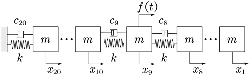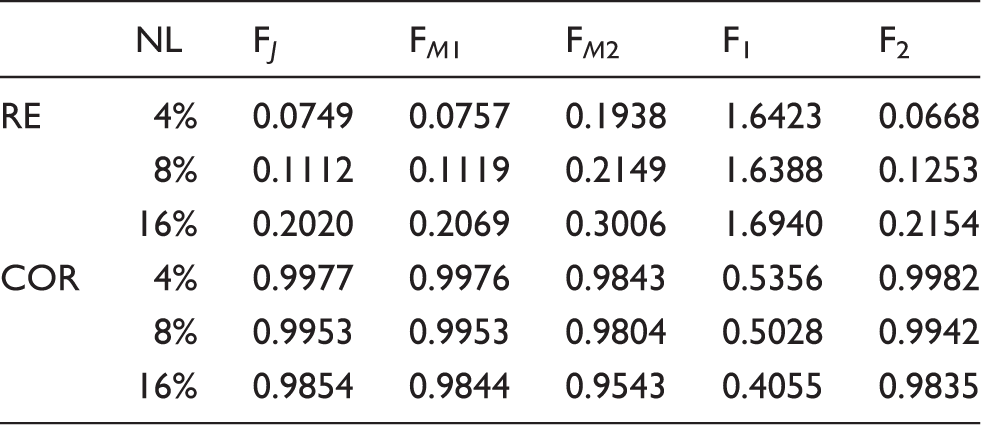The force exerted on x₉ and four accelerometers, located at x₃, x₇, x₁₁ and x₁₅, record the system responses. The undamped natural frequencies of the system are $[0.934, 8.373, 23.077, \dots, 632.89]$ Hz. The sampling frequency f_s is 1024Hz. Three measurement noise levels 4%, 8%, and 16% are considered.

The first case is an impact force. The identification results under different noise levels are shown in Figure 2. The relative errors (REs) and correlations (CORs) are summarized in Table 1.

RE = \frac{‖ F_{identified} - F_{true} ‖_{2}}{‖ F_{true} ‖_{2}}

(64)

COR = \frac{F_{identified}^{T} F_{true}}{‖ F_{identified} ‖_{2} ‖ F_{true} ‖_{2}}

(65)

Table 1.

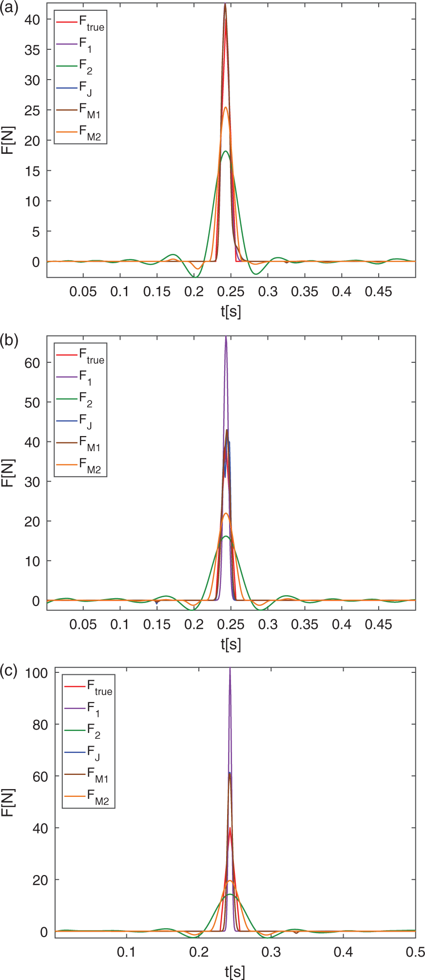
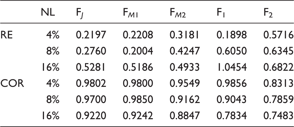
The relative errors (REs) and correlations (CORs) of different estimators of F for the impact force case under different noise levels (NL).

	NL	F _J	F _M ₁	F _M ₂	F₁	F₂
RE	4%	0.2197	0.2208	0.3181	0.1898	0.5716
	8%	0.2760	0.2004	0.4247	0.6050	0.6345
	16%	0.5281	0.5186	0.4933	1.0454	0.6822
COR	4%	0.9802	0.9800	0.9549	0.9856	0.8313
	8%	0.9700	0.9850	0.9162	0.9043	0.7859
	16%	0.9220	0.9242	0.8847	0.7834	0.7483

The final q values of joint PM estimates for the three noise levels are 1.0033, 1.0003 and 1.0046, all close to 1. This indicates that the force is a sparse-type force. When the noise level is 4%, $F_{1}, F_{J}$ and F _M ₁ are very accurate. F₂ underestimates the impact amplitude due to the smoothing effect of Tikhonov regularization. F _M ₂ compulsively considers a wide range of qs. So, sparsity-inducing and smoothing effects are synthesized. F _M ₂ in this case is better than F₂ but worse than F _J and F _M ₁. As the noise level increases to 8%, F₁ though still yields a sparse-type identification, overestimates the impact force amplitude. The results of $F_{J}, F_{M 1}, F_{M 2}$ and F₂ are pretty much same to those under 4% noise level. When the noise level becomes rather large (16%), $F_{1}, F_{J}$ and F _M ₁ all overestimate the impact amplitude. As the noise level increases from 8% to 16%, the REs of $F_{J}, F_{M 1}$ and F₁ increase by 25%, 21% and 40% respectively, while the RE of F _M ₂ only increases by 7%. So F _M ₂ is considered more robust against noise levels, although it is less accurate than F _J and F _M ₁ under 4% and 8% noise.

Note although the REs of $F_{J}, F_{M 1}$ and F _M ₂ become large when the noise level becomes very large (16%), the CORs stay relatively high (92%, 92%, and 88% respectively). This indicates that the true force shape is well identified, but the identified force amplitudes may be erroneous. While for F₂, the RE is high and COR is low, indicating that both the force shape and amplitude are unsatisfactorily identified. So, for this impact force case, we can conclude that F₂ is not an appropriate identification method since Tikhonov regularization has a smoothing effect. F _J and F _M ₁ provide satisfactory identification results with a data-driven automatic determination of q.

The second case is a low-frequency force. The identification results under different noise levels are shown in Figure 3. The RE and COR are summarized in Table 2. The final q values of joint PM estimates for the three noise levels are all 2. In all noise levels, $F_{J}, F_{M 1}$ and F₂ are all similar and satisfactory. Their CORs are all above 98%. F _M ₂ is also considered a good estimate, although the REs are generally higher than F _J and F _M ₁. Unlike the previous impact force case, this time F₂ is a satisfactory identification method. The smoothing effect of Tikhonov regularization well suits the force profile. On the contrary, F₁ has high REs and low CORs, indicating that the force shape and amplitude are both poorly identified. The results highlight the necessity of the adaptive determination of q.

Table 2.

The relative errors (RE) and correlations (COR) of different estimators of 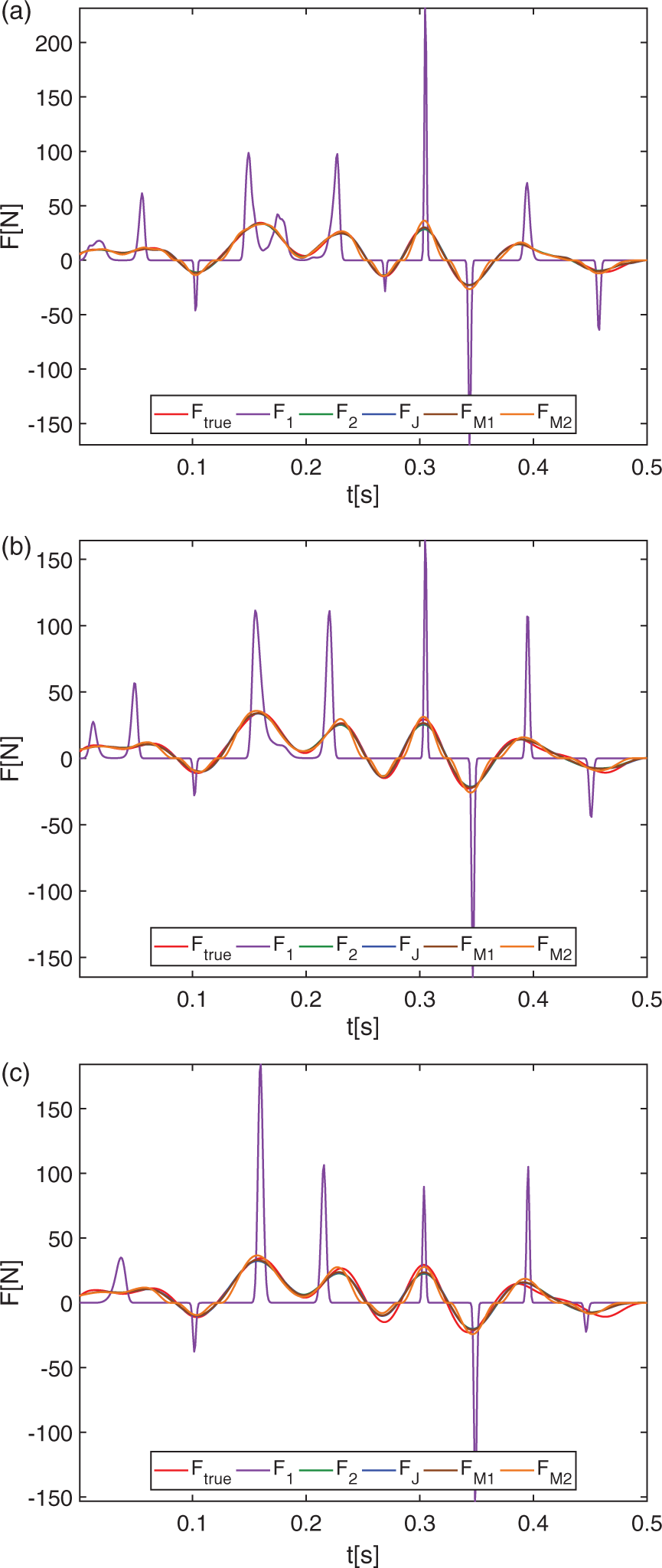F for the low-frequency force case under different noise levels (NL).

	NL	F _J	F _M ₁	F _M ₂	F₁	F₂
RE	4%	0.0749	0.0757	0.1938	1.6423	0.0668
	8%	0.1112	0.1119	0.2149	1.6388	0.1253
	16%	0.2020	0.2069	0.3006	1.6940	0.2154
COR	4%	0.9977	0.9976	0.9843	0.5356	0.9982
	8%	0.9953	0.9953	0.9804	0.5028	0.9942
	16%	0.9854	0.9844	0.9543	0.4055	0.9835

In the above cases, F _M ₁ generally is more accurate than F _M ₂. F _M ₁ calculated

p (q | F^{old}, X)

in a data-driven manner, while F _M ₂ compulsively (inaccurately) sets

p (q | F^{old}, X) = 1

. However, due to the data-driven determination of

p (q | F^{old}, X)

(equivalently a_i), F _M ₂ is generally more computationally intensive than F _M ₁. The computation times for different estimators are summarized in Table 3. Note that these values may vary due to different noise realizations. For the impact force case, the computation times of F _M ₁ are much larger than those of the other two methods. The computation efficiency of F _M ₂ over F _M ₁ is exaggerated.

Table 3.

The computation times (s). Number of q segments N = 100.

	NL	F _J	F _M ₁	F _M ₂
Impact force	4%	18.90	79.39	9.86
	8%	20.64	78.45	9.62
	16%	19.03	87.14	10.01
Low-frequency force	4%	0.35	4.90	6.17
	8%	0.36	5.20	6.70
	16%	0.35	4.60	7.23

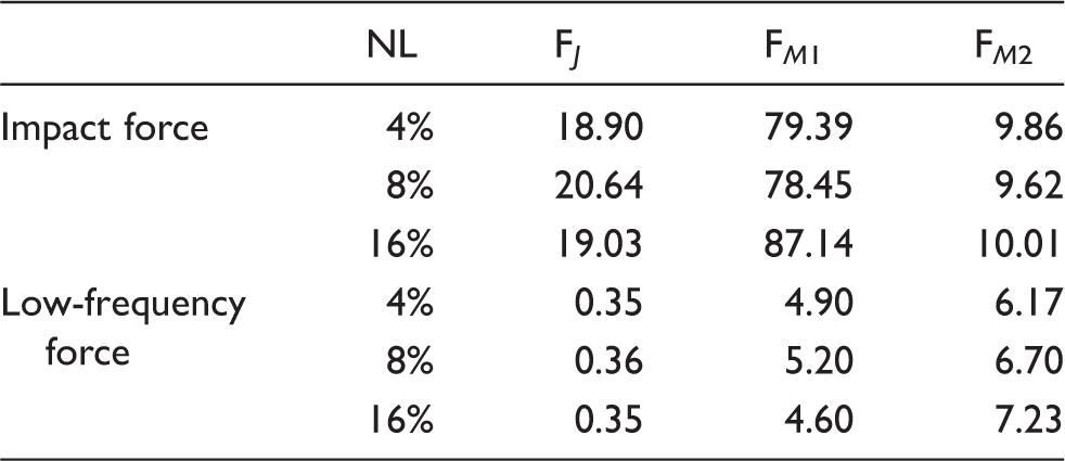
For the low-frequency force case, the computation times of the three methods are respectively much shorter than those of the impact force case. This is due to the fact that $F^{(0)}$ is the result of Tikhonov regularization, which is already a good estimate for the low-frequency force case. While for the impact force case, more iteration steps are needed for convergence. Note that the computation time does not include the time for initialization (Tikhonov regularization with L-curve criterion, typically takes 0.23 s). All the computation is done on a Xeon central processing unit, 16GB RAM personal computer.

4.2. Support structure simulation

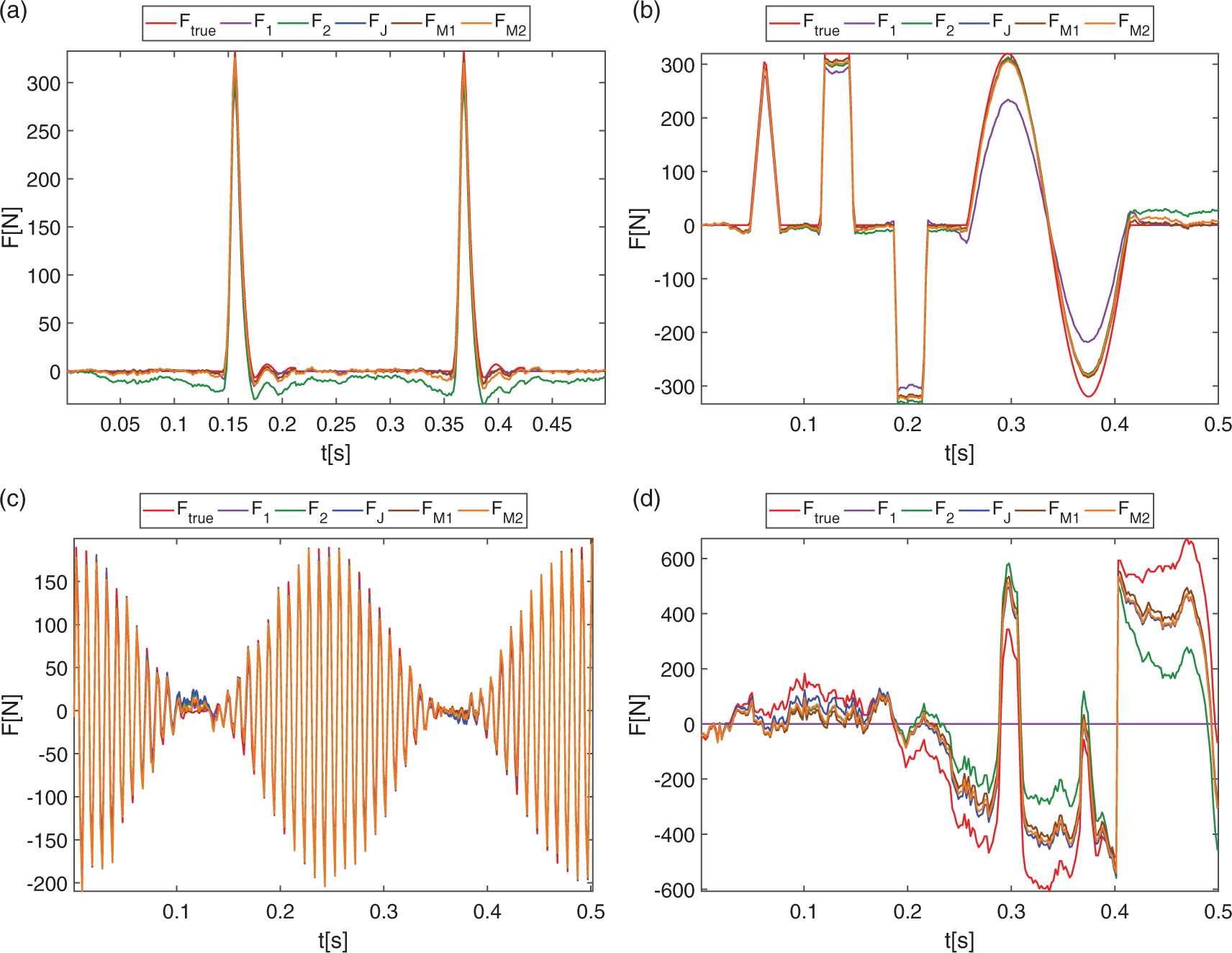
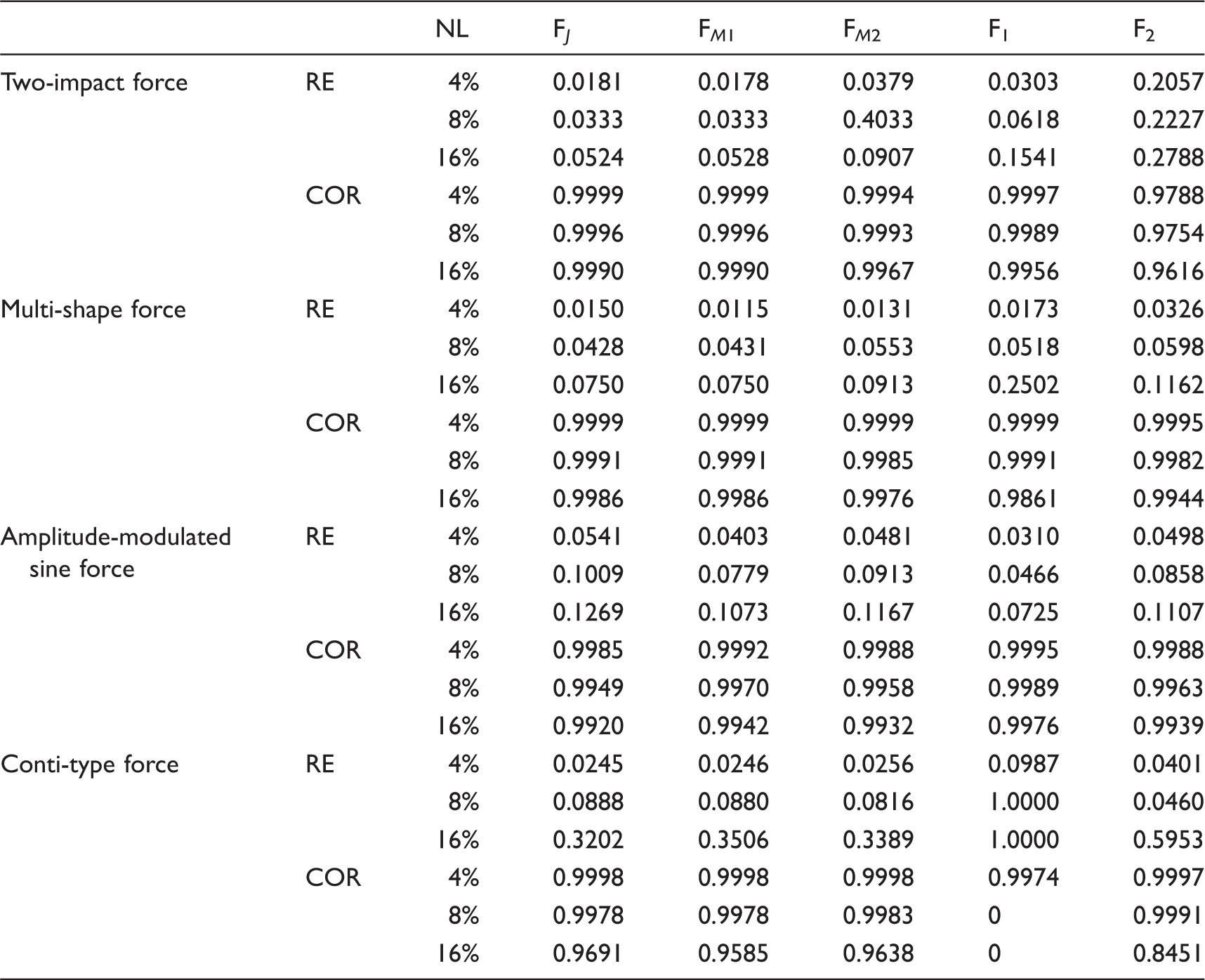
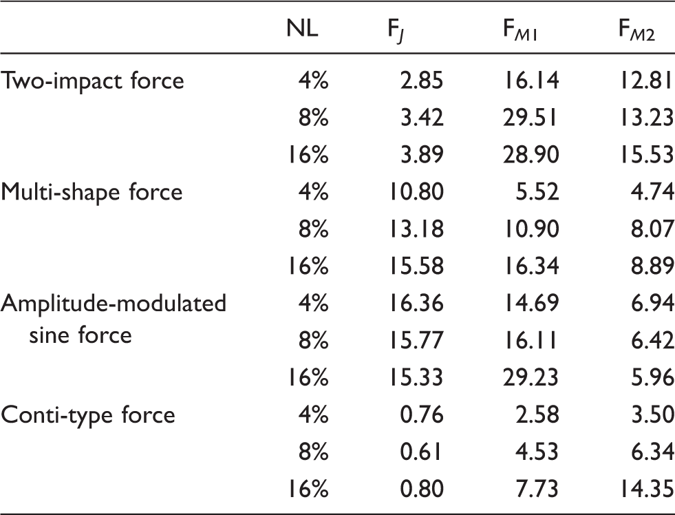
In this section, an engineering scale support structure is studied. The structure is shown in Figure 4. The material properties are Young’s modulus $2 \times 10^{5}$ MPa, density 7850 kg/ $m^{3}$ and Poisson’s ratio 0.3. The structure is meshed with a total of 7146 solid-shell elements (16220 nodes). The first three natural frequencies of the structure are 455.92, 506.07 and 681.47 Hz. A single concentrated force is acting perpendicular to the top surface of the support plane in the y direction. Four uniaxial accelerometers are attached to the bottom surface of the support plane to measure the responses in the y direction. The Rayleigh damping model is assumed and $ζ = 0.02$ is set for the first two modes. Four types of force are studied: a two-impact force; a multi-shape force; an amplitude-modulated sine force; and a continuous-type force. Three noise-levels 4%, 8% and 16% are considered. The identification results of different methods for the forces under noise level 16% are shown in Figure 5. The REs and CORs under different noise levels are summarized in Table 4. In these cases, F _J and F _M ₁ consistently serve as robust estimates of F. F _M ₂, though not as accurate as F _M ₁, is generally faster. Refer to Table 5 for details. Traditional methods by fixing the value of q, will not consistently provide satisfactory results in all situations. Note that for the continuous-type force case, the ℓ₁ regularization result is a zero-vector due to an automatically determined large regularization parameter. For ℓ₁ regularization, when the regularization parameter is above a threshold value, the result will be $0$ .

Table 4.

The relative errors (RE) and correlations (COR) of different estimators of F under different noise levels (NL).

		NL	F _J	F _M ₁	F _M ₂	F₁	F₂
Two-impact force	RE	4%	0.0181	0.0178	0.0379	0.0303	0.2057
		8%	0.0333	0.0333	0.4033	0.0618	0.2227
		16%	0.0524	0.0528	0.0907	0.1541	0.2788
	COR	4%	0.9999	0.9999	0.9994	0.9997	0.9788
		8%	0.9996	0.9996	0.9993	0.9989	0.9754
		16%	0.9990	0.9990	0.9967	0.9956	0.9616
Multi-shape force	RE	4%	0.0150	0.0115	0.0131	0.0173	0.0326
		8%	0.0428	0.0431	0.0553	0.0518	0.0598
		16%	0.0750	0.0750	0.0913	0.2502	0.1162
	COR	4%	0.9999	0.9999	0.9999	0.9999	0.9995
		8%	0.9991	0.9991	0.9985	0.9991	0.9982
		16%	0.9986	0.9986	0.9976	0.9861	0.9944
Amplitude-modulated sine force	RE	4%	0.0541	0.0403	0.0481	0.0310	0.0498
		8%	0.1009	0.0779	0.0913	0.0466	0.0858
		16%	0.1269	0.1073	0.1167	0.0725	0.1107
	COR	4%	0.9985	0.9992	0.9988	0.9995	0.9988
		8%	0.9949	0.9970	0.9958	0.9989	0.9963
		16%	0.9920	0.9942	0.9932	0.9976	0.9939
Conti-type force	RE	4%	0.0245	0.0246	0.0256	0.0987	0.0401
		8%	0.0888	0.0880	0.0816	1.0000	0.0460
		16%	0.3202	0.3506	0.3389	1.0000	0.5953
	COR	4%	0.9998	0.9998	0.9998	0.9974	0.9997
		8%	0.9978	0.9978	0.9983	0	0.9991
		16%	0.9691	0.9585	0.9638	0	0.8451

Table 5.

The computation times (s). Number of q segments N = 100.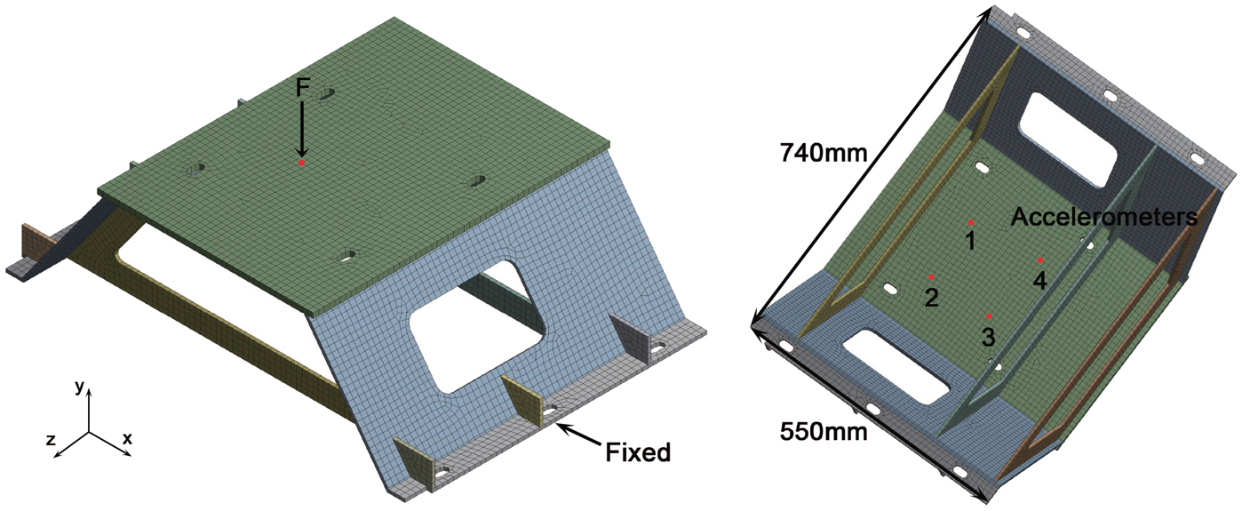

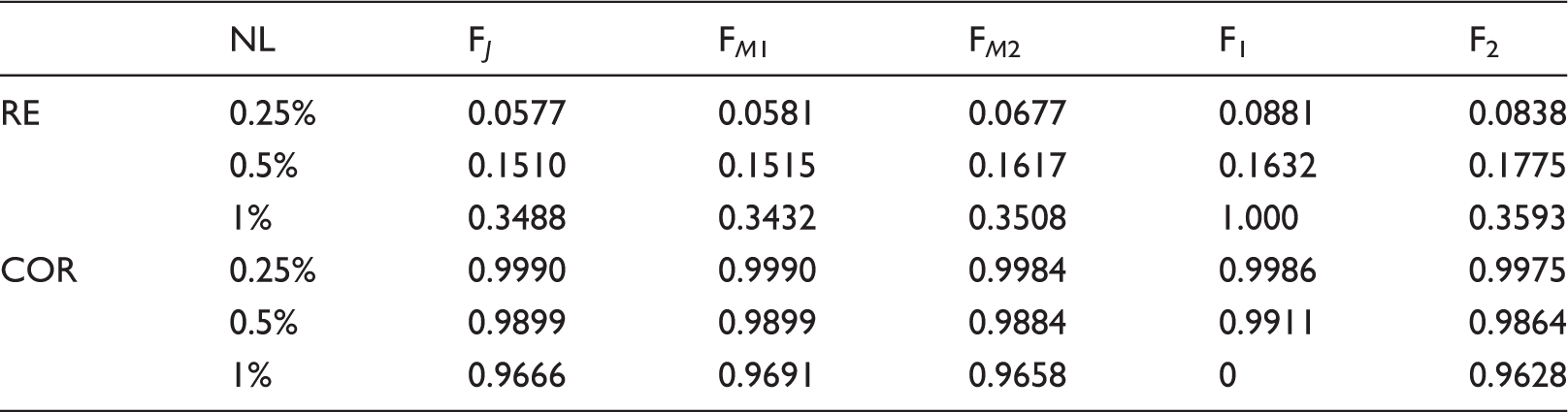
	NL	F _J	F _M ₁	F _M ₂
Two-impact force	4%	2.85	16.14	12.81
	8%	3.42	29.51	13.23
	16%	3.89	28.90	15.53
Multi-shape force	4%	10.80	5.52	4.74
	8%	13.18	10.90	8.07
	16%	15.58	16.34	8.89
Amplitude-modulated sine force	4%	16.36	14.69	6.94
	8%	15.77	16.11	6.42
	16%	15.33	29.23	5.96
Conti-type force	4%	0.76	2.58	3.50
	8%	0.61	4.53	6.34
	16%	0.80	7.73	14.35

In practice, the system unit impulse response function (IRF) is never perfectly known/identified (see the cantilever beam experiment). To validate the stability of the proposed methods in existence of IRF noise, we added different levels of Gaussian white noise into the IRF matrix H of the support structure. The IRF matrix $\bar{H} \in ℝ^{n_{t} \times n_{t}}$ between the force and a certain accelerometer only consists of n_t elements,

\begin{matrix} \bar{H} = [\begin{matrix} h_{1} \\ h_{2} & h_{1} & 0 \\ h_{3} & h_{2} & h_{1} \\ : \\ h_{n_{t}} & \dots & h_{3} & h_{2} & h_{1} \end{matrix}] \end{matrix}

(66)

To simulate the error in system model identification, the vector $h = [h_{1} h_{2} \dots h_{n_{t}}]^{T}$ is added a certain level of Gaussian white noise. The system IRF matrix is reformulated according to the structure in equation (66), with h_i replaced by the polluted ${\tilde{h}}_{i}$ . Here we denote the ith polluted element as ${\tilde{h}}_{i}$ and the reformulated polluted IRF matrix as $\tilde{H}$ . The effect of IRF noise is shown in Figure 6. The true response refers to the real structural response, that is, $\bar{H} F_{true}$ . The measured response equals the true response plus 8% measurement noise. The calculated response refers to $\tilde{H} F_{true}$ ( $F_{true}$ is the multi-shape force. Results of other forces are similar and not presented for brevity). The difference between the true and calculated responses is an intuitive display of the influence of IRF noise. For subfigures (a), (b), and (c), the relative levels of the IRF noise ( $‖ IRFnoise ‖_{2} / ‖ h ‖_{2}$ ) are 0.25%, 0.5%, and 1% respectively. For noise level 0.25%, the polluted IRF $\tilde{H}$ is still very accurate. For noise level 0.5%, the difference between true and calculated responses becomes notable. For even larger noise level 1%, the difference between true and calculated responses is obvious. In practice, such IRF should be considered a failed model identification. The calculated response based on such IRF and precisely recorded force history (for instance by a force transducer), would poorly match the recorded structural response. The REs and CORs of different methods are summarized in Table 6. In these cases, the structural responses are the true structural responses plus 8% measurement noise. Force identification is performed based on the polluted structural response and the polluted system matrix $\tilde{H}$ . It can be seen that, for IRF noise level 0.5%, REs of the proposed methods are still less than 20%. These results validate the stability of the proposed methods in existence of IRF noise.

Table 6.

The relative errors (RE) and correlations (COR) of different estimators of 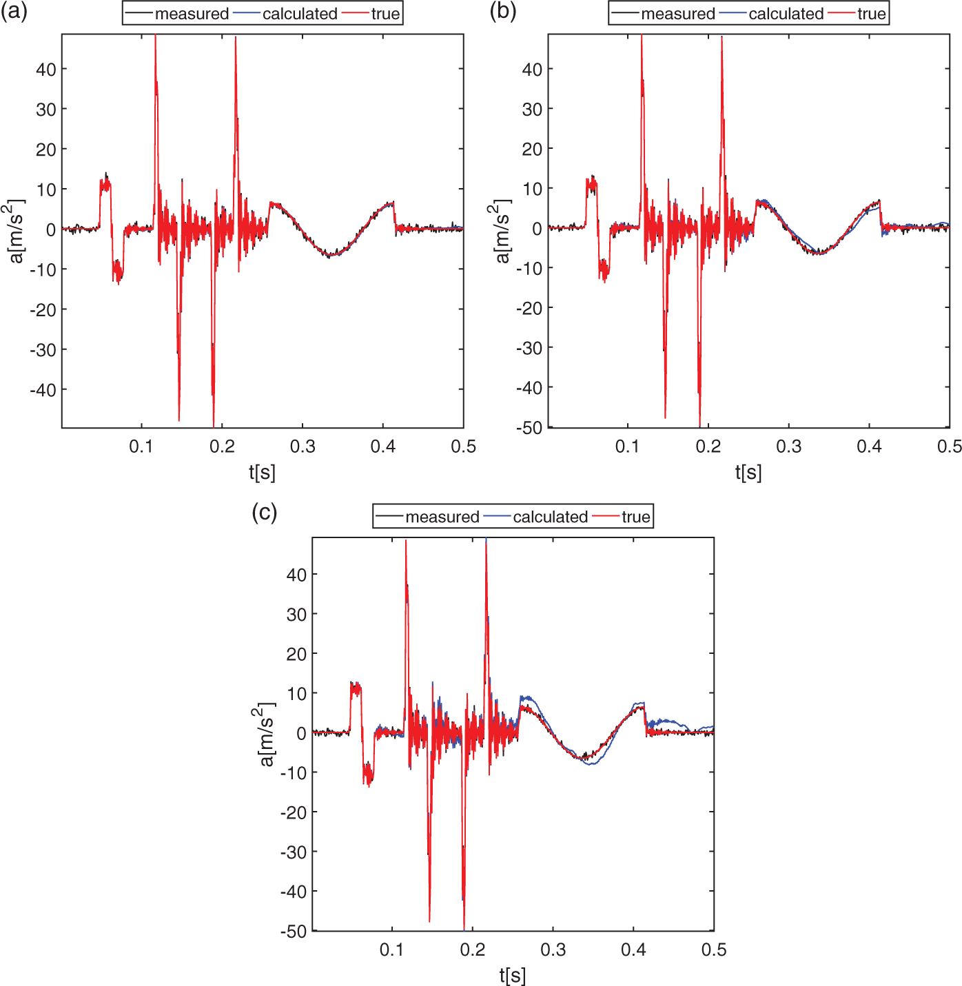F under different impulse response function noise levels (NL). The response measurements are also added 8% noise.

	NL	F _J	F _M ₁	F _M ₂	F₁	F₂
RE	0.25%	0.0577	0.0581	0.0677	0.0881	0.0838
	0.5%	0.1510	0.1515	0.1617	0.1632	0.1775
	1%	0.3488	0.3432	0.3508	1.000	0.3593
COR	0.25%	0.9990	0.9990	0.9984	0.9986	0.9975
	0.5%	0.9899	0.9899	0.9884	0.9911	0.9864
	1%	0.9666	0.9691	0.9658	0	0.9628

4.3. Cantilever beam experiment

In this section, a cantilever beam experiment is carried out to further validate the proposed methods. The experiment configuration is shown in Figure 7. The beam is made of steel and has the dimensions $0.4 \times 0.03 \times 0.01 m^{3}$ . Two accelerometers are mounted on the midline of the beam. A vibration exciter excites the beam at the free end. A programmable signal generator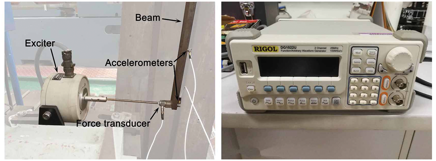 outputs signals of various shapes to the vibration exciter. The excitation force histories are measured by a force transducer. A leuven measurement & system (LMS) is used for data acquisition. The sampling frequency is 8192Hz.

The system IRF matrix is experimentally constructed according to Atobe et al. (2017). The method is briefly described here. Assume we excite the structure N_e times. The measured force histories and responses of a sensor are $F_{e}^{i}$ and $X_{e}^{i} (i = 1, 2, \dots, N_{e})$ . The $F_{e}^{i}$ and $X_{e}^{i}$ are both vectors of length n_e. Then the system IRF coefficient vector can be solved by

h \in ℝ^{n_{e} \times 1} = \min_{h} \sum_{i = 1}^{N_{e}} | | X_{e}^{i} - {\bar{F}}_{e}^{i} h | |_{2}^{2}

(67)

\begin{matrix} {\bar{F}}_{e}^{i} = [\begin{matrix} f_{1}^{i} & 0 \\ f_{2}^{i} & f_{1}^{i} \\ : & : \\ f_{n_{e}}^{i} & f_{n_{e} - 1}^{i} & \dots & f_{1}^{i} \end{matrix}] \end{matrix}

(68)

where

f_{j}^{i}

is the jth element of vector

F_{e}^{i}

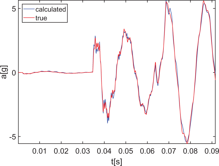
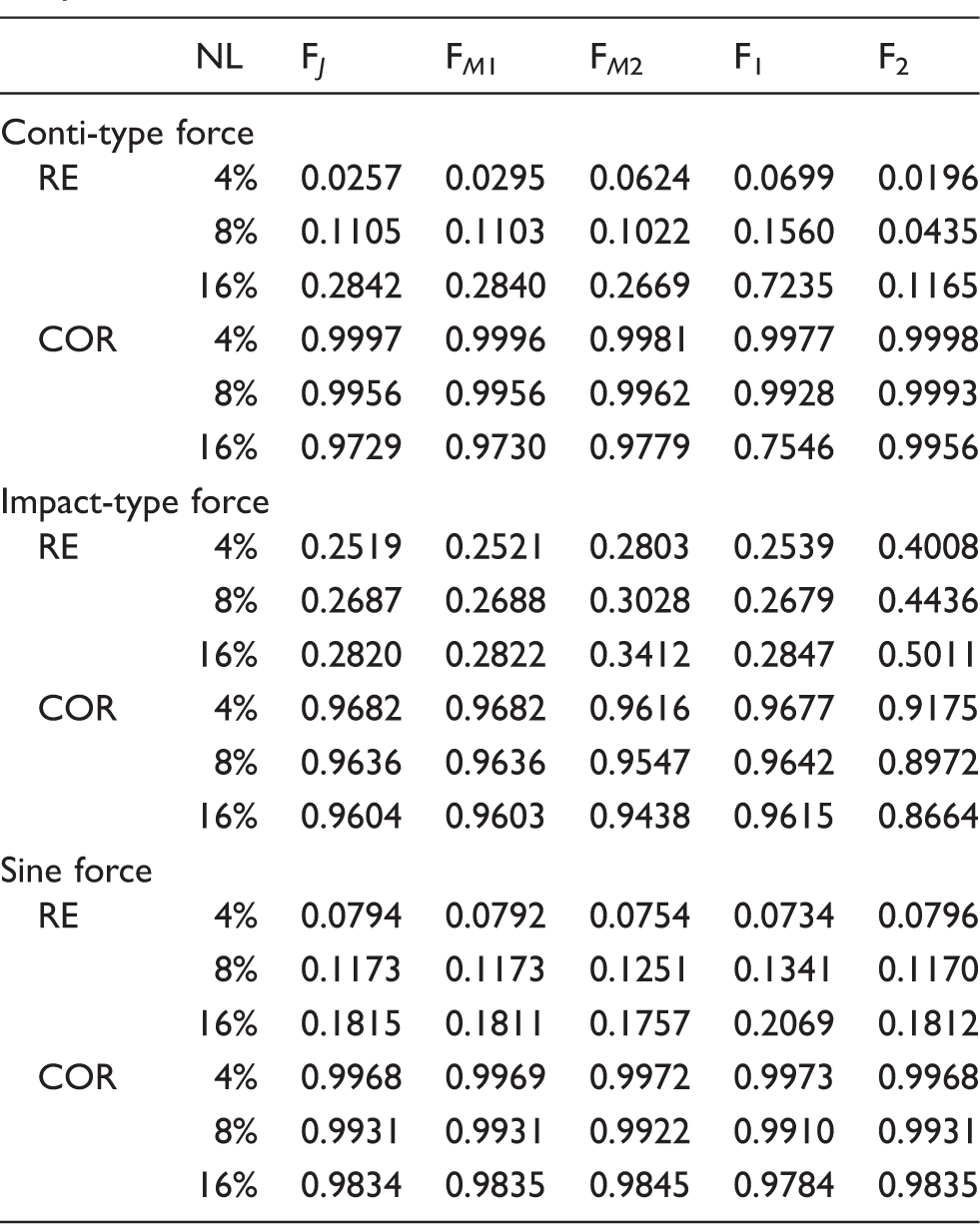
. Then the IRF matrix between the force location and the sensor is constructed according to equation (66). The IRF matrices of two sensors are assembled as the whole system matrix H. Since the identification of h is an optimization problem, the identified result is undoubtedly imperfect. The measured response and the calculated response according to the identified system IRF are shown in Figure 8. It could be seen that a certain amount of error exists in the identified IRF.

Since the laboratory environment is relatively clean, to better study the immunity of the different methods against noise, the recorded responses are added in artificial Gaussian white noise. Three types of forces are studied: a continuous-type force; an impact-type force; and a sine force. Three noise levels are added to the recorded responses: 4%, 8%, and 16%. The identification results based on 16% noise polluted responses are shown in Figure 9. The REs and CORs are summarized in Table 7. It could be concluded that the proposed methods could adapt to the force type and consistently provide satisfactory estimates. Traditional Tikhonov and ℓ₁ regularization methods perform unsteadily in these cases. The results also validate the robustness of the proposed methods to both system IRF noise and measurement noise.

Table 7.

The relative errors (RE) and correlations (COR) of different estimators of 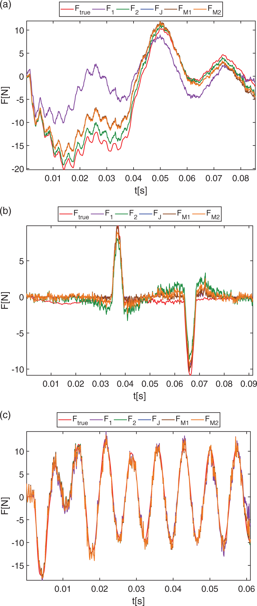F under different noise levels (NL). The impulse response function is experimentally identified. Artificial Gaussian white noise is added to the measurements to simulate noisy environments.

	NL	F _J	F _M ₁	F _M ₂	F₁	F₂
Conti-type force
RE	4%	0.0257	0.0295	0.0624	0.0699	0.0196
	8%	0.1105	0.1103	0.1022	0.1560	0.0435
	16%	0.2842	0.2840	0.2669	0.7235	0.1165
COR	4%	0.9997	0.9996	0.9981	0.9977	0.9998
	8%	0.9956	0.9956	0.9962	0.9928	0.9993
	16%	0.9729	0.9730	0.9779	0.7546	0.9956
Impact-type force
RE	4%	0.2519	0.2521	0.2803	0.2539	0.4008
	8%	0.2687	0.2688	0.3028	0.2679	0.4436
	16%	0.2820	0.2822	0.3412	0.2847	0.5011
COR	4%	0.9682	0.9682	0.9616	0.9677	0.9175
	8%	0.9636	0.9636	0.9547	0.9642	0.8972
	16%	0.9604	0.9603	0.9438	0.9615	0.8664
Sine force
RE	4%	0.0794	0.0792	0.0754	0.0734	0.0796
	8%	0.1173	0.1173	0.1251	0.1341	0.1170
	16%	0.1815	0.1811	0.1757	0.2069	0.1812
COR	4%	0.9968	0.9969	0.9972	0.9973	0.9968
	8%	0.9931	0.9931	0.9922	0.9910	0.9931
	16%	0.9834	0.9835	0.9845	0.9784	0.9835

5. Conclusions

The motivation of this study is to robustly identify the history of an external force acting on structures, by adaptively choosing the appropriate ℓ_q regularization according to the force profile. The choice of q generally has great influence on the identified force history, and is usually considered known a priori in the existing literature. In situations where such information is vague, q needs to be adaptively determined. To achieve this, the inverse force identification problem is first formulated within the Bayesian framework. The joint (F _J ) and marginal (F _M ₁) PMs of the force history are then proposed for its estimation. They are respectively solved by CM and EM algorithms. For computational efficiency, an approximate marginal PM estimator (F _M ₂) is also proposed. For the joint PM estimator, q is iteratively calculated; for marginal PM estimators, q affects in an integral manner. Both numerical and experimental results have highlighted the benefits of the adaptive determination of q. The proposed methods could adapt to the force profile and consistently provide satisfactory identifications. From the validation results, F _J and F _M ₁ estimates are generally similar. F _M ₂ benefits from higher computational efficiency. The proposed methods are also proven stable in existence of both system and measurement noise. Further studies could include the adaptive regularization for multiple forces and sparsity/continuity time-varying forces.

Footnotes

Declaration of Conflicting Interests

The author(s) declared no potential conflicts of interest with respect to the research, authorship, and/or publication of this article.

Funding

The author(s) received no financial support for the research, authorship, and/or publication of this article.

References

Atobe

Nonami

et al. (2017) Identification of impact force acting on composite laminated plates using the radiated sound measured with microphones. Journal of Sound and Vibration 405: 251–268. Available at: https://doi.org/10.1016/j.jsv.2017.06.009.

Aucejo

(2014) Structural source identification using a generalized Tikhonov regularization. Journal of Sound and Vibration 333(22): 5693–5707.

Aucejo

De Smet

(2016) Bayesian source identification using local priors. Mechanical Systems and Signal Processing 66–67: 120–136. Available at: https://doi.org/10.1016/j.ymssp.2015.05.004.

Aucejo M and De Smet O (2017a) Bayesian formulations for force reconstruction problems. In: Proceedings of the 6th International Conference on Computational Methods in Structural Dynamics and Earthquake Engineering, COMPDYN 2017, in conjunction with the 2nd International Conference on Uncertainty Quantification in Computational Sciences and Engineering, UNCECOMP 2017, Rhodes Island, Greece, 15–17 June 2017.

Aucejo

De Smet

(2017b) A multiplicative regularization for force reconstruction. Mechanical Systems and Signal Processing 85: 730–745. Available at: https://doi.org/10.1016/j.ymssp.2016.09.011.

Azam

Chatzi

Papadimitriou

et al. (2015) Experimental validation of the Kalman-type filters for online and real-time state and input estimation. Journal of Vibration and Control 23(15): 2494–2519.

Faure

Ablitzer

Antoni

et al. (2017) Empirical and fully Bayesian approaches for the identification of vibration sources from transverse displacement measurements. Mechanical Systems and Signal Processing 94: 180–201. Availabel at: https://doi.org/10.1016/j.ymssp.2017.02.023.

Feng

Sun

Feng

(2015) Simultaneous identification of bridge structural parameters and vehicle loads. Computers & Structures 157(3): 76–88.

Hansen

(1998) Rank-Deficient and Discrete Ill-Posed Problems: Numerical Aspects of Linear Inversion, Philadelphia, PA: Society for Industrial and Applied Mathematics.

10.

Jacquelin

Bennani

Hamelin

(2003) Force reconstruction: Analysis and regularization of a deconvolution problem. Journal of Sound and Vibration 265(1): 81–107.

11.

(2016) Impact localization and identification under a constrained optimization scheme. Journal of Sound and Vibration 366: 133–148. Available at: https://doi.org/10.1016/j.jsv.2015.12.010.

12.

(2017) Force localization and reconstruction using a two-step iterative approach. Journal of Vibration and Control. E-pub ahead of print 5 July 2017. DOI:10.1177/1077546317713366.

13.

Feng

Chu

(2014) A load identification method based on wavelet multi-resolution analysis. Journal of Sound and Vibration 333(2): 381–91.

14.

Mobayen

(2015) An adaptive fast terminal sliding mode control combined with global sliding mode scheme for tracking control of uncertain nonlinear third-order systems. Nonlinear Dynamics 82(1–2): 599–610.

15.

Mobayen

Javadi

(2016) Disturbance observer and finite-time tracker design of disturbed third-order nonholonomic systems using terminal sliding mode. Journal of Vibration and Control 23(2): 181–189.

16.

Pan

Liu

(2017) Identification of moving vehicle forces on bridge structures via moving average Tikhonov regularization. Smart Materials and Structures 26(8): : 085041. DOI:10.1088/ 1361-665X/aa7a48.

17.

Pan

Liu

et al. (2018) Moving force identification based on redundant concatenated dictionary and weighted l1-norm regularization. Mechanical Systems and Signal Processing 98: 32–49. Available at: https://doi.org/10.1016/j.ymssp.2017.04.032.

18.

Qiao

Zhang

Gao

et al. (2016a) Impact-force sparse reconstruction from highly incomplete and inaccurate measurements. Journal of Sound and Vibration 376: 72–94. Available at: https://doi.org/10.1016/j.jsv.2016.04.040.

19.

Qiao

Zhang

Wang

et al. (2016b) Sparse regularization for force identification using dictionaries. Journal of Sound and Vibration 368: 71–86. Available at: https://doi.org/10.1016/j.jsv.2016.01.030.

20.

Qiao

Xingwu

Jiawei

et al. (2017) Sparse deconvolution for the large-scale ill-posed inverse problem of impact force reconstruction. Mechanical Systems and Signal Processing 83: 93–115. Available at: https://doi.org/10.1016/j.ymssp.2016.05.046.

21.

Ronasi

Johansson

Larsson

(2011) A numerical framework for load identification and regularization with application to rolling disc problem. Computers & Structures 89(1–2): 38–47.

22.

Samagassi

Khamlichi

Driouach

et al. (2015) Reconstruction of multiple impact forces by wavelet relevance vector machine approach. Journal of Sound and Vibration 359: 56–67. Available at: https://doi.org/10.1016/j.jsv.2015.08.014.

23.

Sun

Büyüköztürk

(2015) Identification of traffic-induced nodal excitations of truss bridges through heterogeneous data fusion. Smart Materials and Structures 24(7): : 075032. DOI:10.1088/ 0964-1726/24/7/075032.

24.

Vogel

(2011) Computational Methods for Inverse Problems, 2nd ed. Beijing: Tsinghua University Press.

25.

Wentzel

(2013) Fatigue test load identification using weighted modal filtering based on stress. Mechanical Systems and Signal Processing 40(2): 618–627.

26.

Yan

Sun

Büyüköztürk

(2017) Impact load identification for composite structures using Bayesian regularization and unscented Kalman filter. Structural Control and Health Monitoring 24(5): : e1910–n/a. DOI:10.1002/stc.1910.