Tubing leak detection for wellbore leak localization: A coupled flow-acoustic simulation approach

Abstract

Wellbore tubing leakage poses severe threats to the operational safety and resource efficiency of oil and gas exploitation, and existing research suffers from insufficient understanding of flow-acoustic coupling mechanisms, lack of systematic analysis of multi-factor interactions, and oversimplified acoustic propagation models. To address these limitations, this study develops a bidirectional coupled flow-acoustic model matching the actual structural characteristics of wellbores, and conducts systematic simulations under adiabatic conditions considering different pressure differences (1–3 MPa), orifice diameters (1–5 mm), and three orifice shapes. Flow field results reveal that the fluid passing through the leak orifice exhibits a distinct “pressure drop-velocity increase” characteristic, with both pressure difference and orifice diameter exerting significant regulatory effects on fluid density and velocity distributions. Acoustic field results demonstrate a “laminar-like” distribution pattern of acoustic waves in the tubing; an increase in pressure difference elevates the sound pressure level (SPL) of leakage noise without causing peak frequency shift, while an increase in orifice diameter not only raises the SPL but also induces a significant shift in the peak frequency of the acoustic spectrum. This study further derives quantitative correlation formulas between SPL and pressure difference/orifice diameter, as well as between spectral peak frequency and orifice diameter, realizing the inversion of leakage working conditions from acoustic signals. The research findings optimize the non-intrusive leakage detection technology for high temperature-high pressure (HTHP) and high-sulfur wells, and provide a novel theoretical and technical basis for accurate wellbore leak localization.

Keywords

wellbore tubing leakage flow field-acoustic field coupled simulation non-intrusive detection sound pressure level LES turbulence model

1. Introduction

Wellbore tubing leakage in oil and gas exploitation jeopardizes operational safety, leading to resource loss, wellbore integrity failures like annular pressure buildup (APB) and casing corrosion, and hazardous releases causing environmental pollution or blowouts. In HTHP/high-sulfur environments, leakage is mainly caused by corrosion and material failures, such as hydrogen embrittlement (Al-Zahrani et al., 2024; Ogunlakin et al., 2026), flow accelerated corrosion (FAC) (Toor et al., 2020), microbiological corrosion (Amiri et al., 2024; Arrousasi et al., 2025), and stress corrosion cracking, which complicate detection due to diverse and coupled effects. Research on mechanisms, factors, and detection is vital. Non-intrusive detection is mainstream to avoid production disruption, supported by flow field-acoustic simulation for feature characterization and accuracy.

Early studies focused on causes, patterns, and coupling effects. Wojtanowicz et al. (2001) linked tubing leakage to APB via statistics, associating it with temperature fluctuations, pressure cycles, and material degradation. Kutchko (2008) showed cement sheath defects exacerbate leakage by enabling fluid channeling and pressure differentials. William Carey et al. (2009) found leakage severity depends on channel size: diffusion-dominated for 50–150 μm and flow-driven expansion for larger channels. Huerta et al. (2009) developed an APB model considering leakage location, orifice size, and formation pressure, while Rocha-Valadez et al. (2014) highlighted H₂S accelerating stress corrosion cracking, enlarging orifices by 30–50%, and creating a leakage-corrosion cycle. With digitization, AI/ML technologies (Allah, 2025) are increasingly used for intelligent feature extraction, noise reduction, and leakage location in acoustic/flow signals, enhancing detection efficiency and accuracy in complex corrosion conditions.

For complex conditions like HTHP and high sulfur, mechanistic understanding improved. Tao et al. (2010) linked APB recovery to cement permeability: >100 mD aids detection, and <10 mD causes hidden leakage. Zhou et al. (2018) enhanced models with non-Newtonian fluids, finding flow index and mud length key for leakage prediction in high-sulfur wells. Numerical modeling is key for corrosion-induced leakage in HTHP, particularly FAC (Al-Abed Allah et al., 2026; Meri et al., 2025), simulating fluid-corrosion coupling, quantifying wall thinning and micro-leakage, and enabling early warning. Leakage has multi-dimensional impacts: Xu et al. (2017) found gas leakage disrupts phase balance, exceeding pressure limits. Eulberg et al. (2017) showed leaked fluids cause temperature swings, increasing thermal stress via a leakage-temperature deformation chain. In high-sulfur HTHP wells, Lian et al. (2023) and Zhou et al. (2023) noted leakage creates low-pressure zones or high radial pressure, leading to cycles that shorten well life or cause blowouts. Corrosion-induced failure combined with environmental factors complicates leakage flow-acoustic characterization, demanding higher accuracy in numerical models.

Traditional detection has limitations: intrusive methods stop production and risk damage, while non-intrusive ones lack accuracy in complex corrosion conditions. Flow-acoustic coupling is a key non-intrusive solution. Early work on acoustic basics: Hunaidi et al. (1999) studied leakage sounds and built systems. Kim et al. (2009) modeled sound propagation with BEM for wellbores. Advanced simulations enabled deeper coupling: Chen et al. (2017) combined CFD and heat transfer to locate leaks. Xiao et al. (2019) created a wavelet-SVM model with 99.4% accuracy. For complex cases, Wu et al. (2018) reached 99.32% accuracy for sub-liquid leakage by connecting bubble dynamics to sound. Yang et al. (2022) made a MAWF model with 98.79% accuracy for offshore wells. To reduce noise, Yao et al. (2023) added noise separation, achieving 95.17% fault accuracy with FAE-1D-CNN. Zhang et al. (2025) boosted positioning accuracy using CFD fluid data, cutting error to <1.8%. However, most flow-acoustic models lack corrosion-induced orifice evolution data, limiting use in real HTHP/high-sulfur wells with complex corrosion.

However, most flow-acoustic models lack corrosion-induced orifice evolution data, limiting use in real HTHP/high-sulfur wells with complex corrosion. Existing typical studies (Wu et al., 2018; Yang et al., 2022) mainly focus on leakage localization accuracy and multi-feature fusion identification, but rarely reveal the inherent turbulent-acoustic coupling mechanism inside the leakage orifice, nor establish quantitative relations between sound pressure level (SPL), spectral peak frequency, pressure difference, and orifice diameter. Moreover, the “laminar-like” acoustic propagation pattern inside tubing and its physical origin have not been reported.

To address these gaps, a multi-software framework with SolidWorks, ICEM, Fluent, and ACTRAN is used to develop a full-scale flow-acoustic coupling model for gas well tubing-casing annular leakage. The model employs LES and Lighthill analogy for bidirectional coupling, accurately reproducing turbulent jet evolution, acoustic generation, and wave propagation in multi-medium wellbores. It analyzes flow and acoustic field evolution under different pressures and diameters, revealing the “laminar-like” acoustic distribution mechanism and establishing quantitative flow-acoustic correlations. Compared with Wu et al. (2018) and Yang et al. (2022), this study not only improves localization accuracy but also clarifies the generation mechanism of leakage noise, realizes quantitative inversion of leakage parameters, and proposes an adaptive frequency strategy suitable for HTHP and high-sulfur wells. Results enrich downhole leakage theory and provide optimization schemes for non-intrusive acoustic detection, enhancing leak detection accuracy, well safety, and reducing resource loss.

2. Model and equation

Natural gas influx into the annulus caused by tubing leakage typically generates abnormal pressure that threatens gas well production, making rapid and accurate leakage detection imperative. Therefore, analyzing the flow field and acoustic characteristics of tubing leakage is critical for guiding the optimization of detection equipment. This study adopts a two-step approach for acoustic field simulation of tubing leakage in gas production wells—first simulating the flow field and then calculating the acoustic field—and conducts numerical simulations of the flow and acoustic fields under different operating conditions based on relevant theoretical foundations, thereby laying the groundwork for ultrasonic detection method application. Building on theoretical analyses, the study employs Fluent to simulate the leakage flow field and analyze the impacts of related factors, and further performs coupled acoustic field simulations via Fluent and ACTRAN to explore sound source characteristics. Significantly, the flow field theories associated with leakage are established in previous research (Kuanhai et al., 2020; Meng et al., 2021; Tian et al., 2023), while the detailed sound field modeling process is provided in the supplementary file.

In addition, to enhance the clarity of the main text and highlight core research findings, detailed technical details including Model Assumptions, Turbulence Modeling Strategy, Geometric Model and Mesh, Boundary Condition, and Flow-Acoustic Coupling Transition Mechanism have been systematically organized in Appendix 2 for readers requiring in-depth technical references.

3. Results and discussion

3.1. Analysis of oil pipe leakage flow field simulation results

3.1.1. Analysis of tubing leakage flow field

Based on the flow field simulation theory, the tubing-casing leakage flow field model is imported into simulation software for flow field calculation. First, a standard k-ε turbulence model is used to calculate the steady-state flow field of tubing-casing leakage—this step aims to quickly obtain the basic flow structure and provide a convergent initial condition for the subsequent LES transient simulation. Direct transient simulation of complex leakage turbulence via LES without steady-state initialization is prone to numerical oscillation or non-convergence, which significantly reduces computational efficiency and result reliability. Since the simulation of the casing micro-leakage flow field focuses on the intense turbulent flow at and near the leak hole, images such as velocity contour maps and pressure contour maps in this study are all magnified views of the area around the leak hole. After obtaining the steady-state flow field via the k-ε model, the LES model is used for transient calculation to capture the unsteady turbulent details that determine the acoustic source characteristics. The transient flow field results are presented in Sections 3.1.2 and 3.1.3.

Numerical simulation is conducted under the working condition where the tubing pressure is 8 MPa, the casing outlet pressure is 6 MPa, and the leak hole size is 3 mm. As shown in Figure 1, the pressure inside the casing annulus remains basically constant, indicating that the impact of the leakage process on the internal pressure of the annulus is negligible. Similarly, at the inlet of the leak hole, the pressure begins to change, and the pressure gradient reaches its maximum—this phenomenon indicates intense fluid disturbance at the leak hole inlet. The pressure near the leak orifice drops rapidly from 8 MPa to 5–6 MPa, and the fluid pressure decreases gradually along the leak hole.

Figure 1.

Oil pipe leakage pressure cloud map.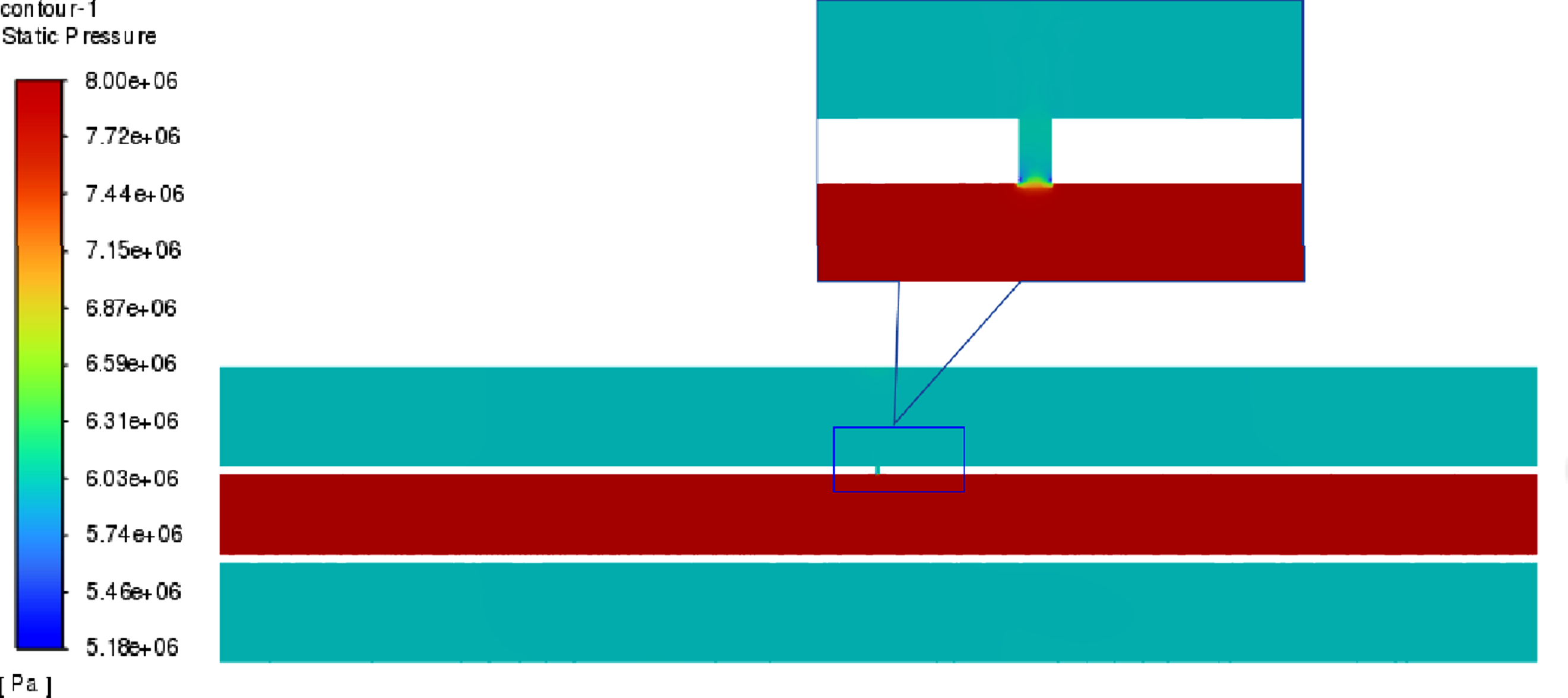

As shown in Figure 2, there is almost no disturbance in the fluid flow inside the casing annulus, with the fluid velocity being zero. However, near the inlet of the leak hole, the fluid begins to flow under the action of the pressure difference between the inside and outside of the casing.

Figure 2.

Oil pipeline leakage rate cloud map.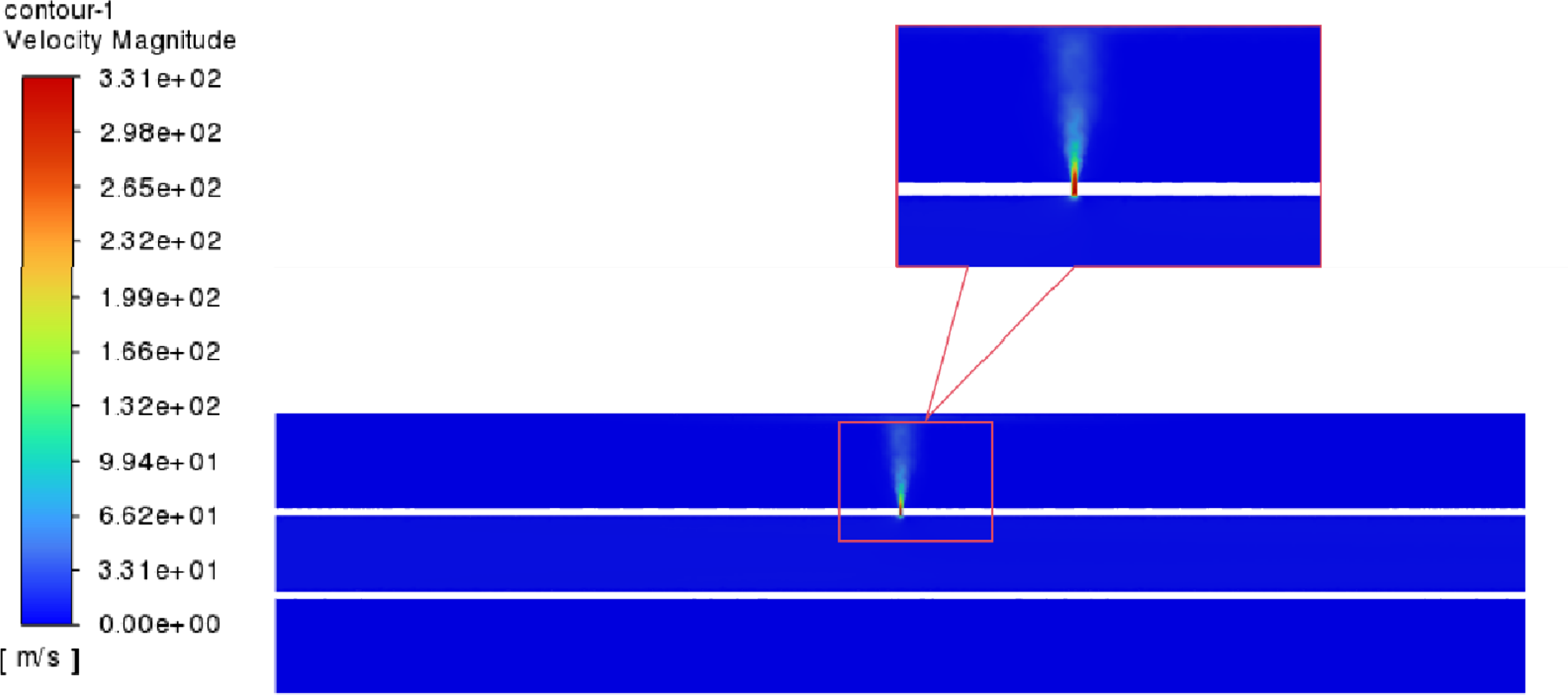

The color gradient is the largest at the leak hole inlet—that is, the junction of the leak hole and the casing—which indicates the most intense flow field disturbance at this location. Inside the leak hole, the fluid velocity increases gradually and reaches a maximum of 331 m/s at the top of the leak hole. Additionally, the fluid velocity increases as the distance from the leak hole axis decreases, achieving its maximum value along the leak hole axis.

Figure 5 shows the pressure distribution and velocity distribution curves along the leak hole axis, respectively. As indicated in Figure 5(a) and (b), the fluid pressure and velocity undergo intense changes near the inlet and outlet of the leak hole, making this region the one with the largest gradients in the entire flow field.

Notably, the fluid pressure and velocity begin to change even before the fluid enters the leak hole. After entering the leak hole, the fluid velocity first decreases and then increases. This phenomenon occurs because when the fluid flows from the tubing into the leak hole, the cross-sectional area shrinks suddenly, leading to the contraction of the fluid stream in the leak hole and a subsequent decrease in fluid velocity. Thereafter, the fluid pressure drops and the velocity increases continuously inside the leak hole, resulting in a gradual rise in flow velocity.

The fluid velocity reaches its maximum outside the leak hole outlet. This is because after the fluid flows out of the leak hole, its pressure is still higher than the annulus pressure, leading to further expansion. Correspondingly, the fluid velocity increases accordingly. At the same time, the rapid expansion of the fluid generates a shock wave—a type of compression wave—that causes a sudden increase in fluid pressure, as shown in Figure 3. Subsequently, the fluid pressure approaches the annulus pressure and remains constant. In the annulus, the fluid velocity gradually decreases due to the interaction between the stationary air and the fluid.

Figure 3.

Pressure distribution and velocity distribution curves along the leak hole axis: (a) velocity distribution and (b) pressure distribution.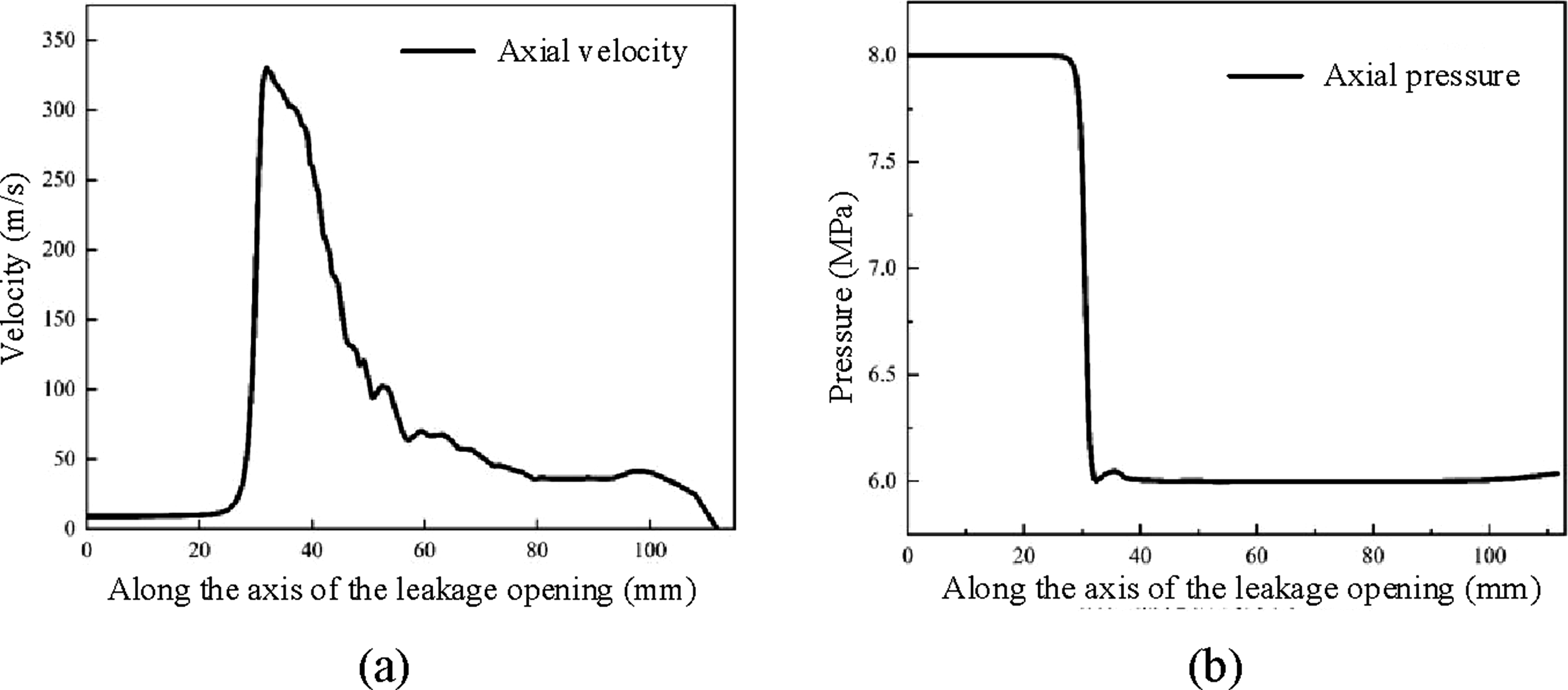

When the tubing pressure is 8 MPa, casing outlet pressure is 6 MPa, and leak hole diameter is 3 mm, According to the calculation method in references [13,17], the turbulence intensity near the orifice reaches 0.42 (dimensionless), vorticity peaks at 1.1 × 10⁵ rad/s, and turbulent kinetic energy k is 3.6 × 10⁴ m²/s². According to the Lighthill analogy, the quadrupole source term $T_{i j} = ρ u_{i} u_{j} - τ_{i j}$ is dominated by momentum flux $ρ u_{i} u_{j}$ (accounting for 92% of $T_{i j}$ ), confirming that turbulent momentum transfer in the flow field is the primary driver of leakage acoustic signals.

Additionally, as can be seen from Figures 1 –5, the fluid velocity is relatively high in the entire noise source region. In this case, the quadrupole sound power of the fluid is much higher than the dipole sound power. Therefore, it is reasonable to conclude that the noise generated by pipeline leakage is mainly caused by the quadrupole sound source of fluid flow.

3.1.2. Effect of casing pressure difference on leakage flow field

The LES turbulence model was selected for the transient calculation of the flow field. Meanwhile, to investigate the influence of different pressure differences between the inside and outside of the casing on the leakage flow field, transient flow field simulations were conducted for tubing leakage conditions with a leak hole size of 0.2 mm and pressure differences of 1 MPa, 1.5 MPa, 2 MPa, 2.5 MPa, and 3 MPa between the inside and outside of the casing.

Figure 4 shows the density distribution along the leak hole axis under different pressure differences. As observed in Figure 4(a), the fluid density changes drastically near the leak hole inlet, with a decrease in density. The larger the pressure difference, the greater the density gradient. Inside the leak hole, the fluid density continues to decrease, and similarly, the larger the pressure difference, the greater the gradient. At the leak hole outlet, the density under a pressure difference of 3 MPa is still higher than that under 1 MPa. In the core region of the jet outside the leak hole, the fluid density rises suddenly due to the generation of shock waves. The larger the pressure difference, the greater the rise value. Thereafter, the fluid density decreases gradually and finally stabilizes.

Figure 4.

Density and axial velocity variation of fluid along the axis of leakage hole under different pressure difference: (a) density distribution along the leakage hole axis and (b) axial velocity distribution along the leakage hole axis.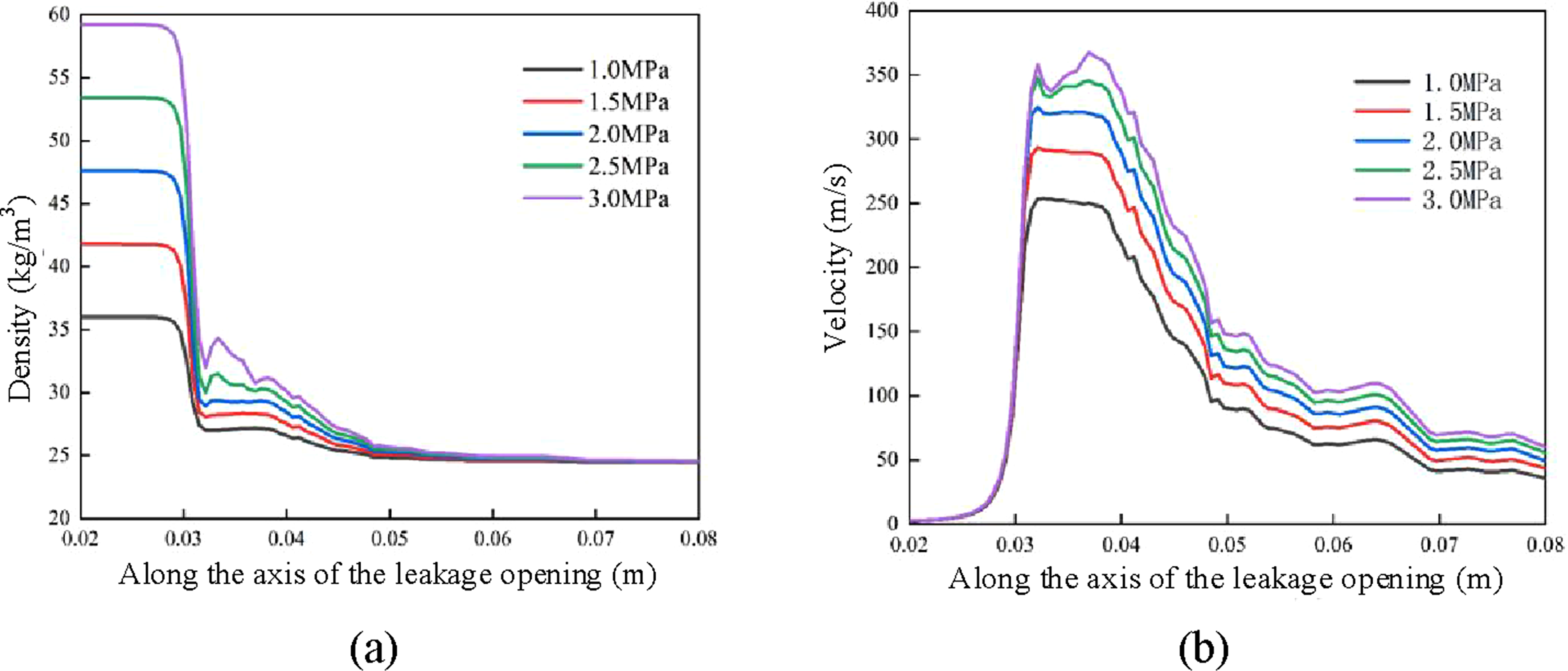

Figure 4(b) presents the velocity distribution along the leak hole axis under different pressure differences. As observed in Figure 4(b), inside the tubing, the pressure difference has almost no effect on the fluid velocity. Near the leak hole inlet, the fluid velocity begins to be affected by the pressure difference and surges rapidly, with the velocity growth trend being consistent across different pressure differences. Differences emerge at the leak hole outlet: the velocity gradient increases as the pressure difference rises. In the core region of the jet, the fluid velocity reaches its maximum value, and this maximum value increases with the increase in pressure difference. Finally, as the fluid continues to jet outward, the velocity decreases.

Analysis of the two diagrams reveals that within the leakage hole, fluid density increases proportionally with the pressure differential, while flow velocity remains relatively constant, with variations occurring only near the outlet. In the annular space, fluid density shows minimal change with increasing pressure differential, whereas flow velocity rises significantly.

Given that acoustic power from the source is directly proportional to fluid density and velocity, it follows that both the leakage hole and annular space exhibit greater acoustic intensity as the pressure differential increases.

As the pressure difference increases from 1 MPa to 3 MPa, the turbulent kinetic energy k near the orifice rises from 1.8 × 10⁴ m²/s² to 6.3 × 10⁴ m²/s², which enhances the acoustic source term by 250%. This quantitative correlation explains the linear growth of SPL observed in the subsequent acoustic simulation (Section 3.2.2), as the intensified turbulent fluctuations directly amplify the strength of the acoustic source.

3.1.3. Effect of different leakage pore size on leakage flow field

To investigate the influence of leak hole size on the flow field, numerical simulations were conducted on tubing models with different leak hole sizes. The pressure difference was fixed at 2 MPa, and the leak hole sizes were set to 1 mm, 2 mm, 3 mm, 4 mm, and 5 mm, respectively.

Figure 5 shows the density distribution and velocity distribution along the leak hole axis under different leak hole sizes, respectively.

Figure 5.

Density and velocity variation along the leakage hole axis at different pore sizes: (a) fluid density distribution along the leakage hole axis and (b) fluid velocity distribution along the leakage hole axis.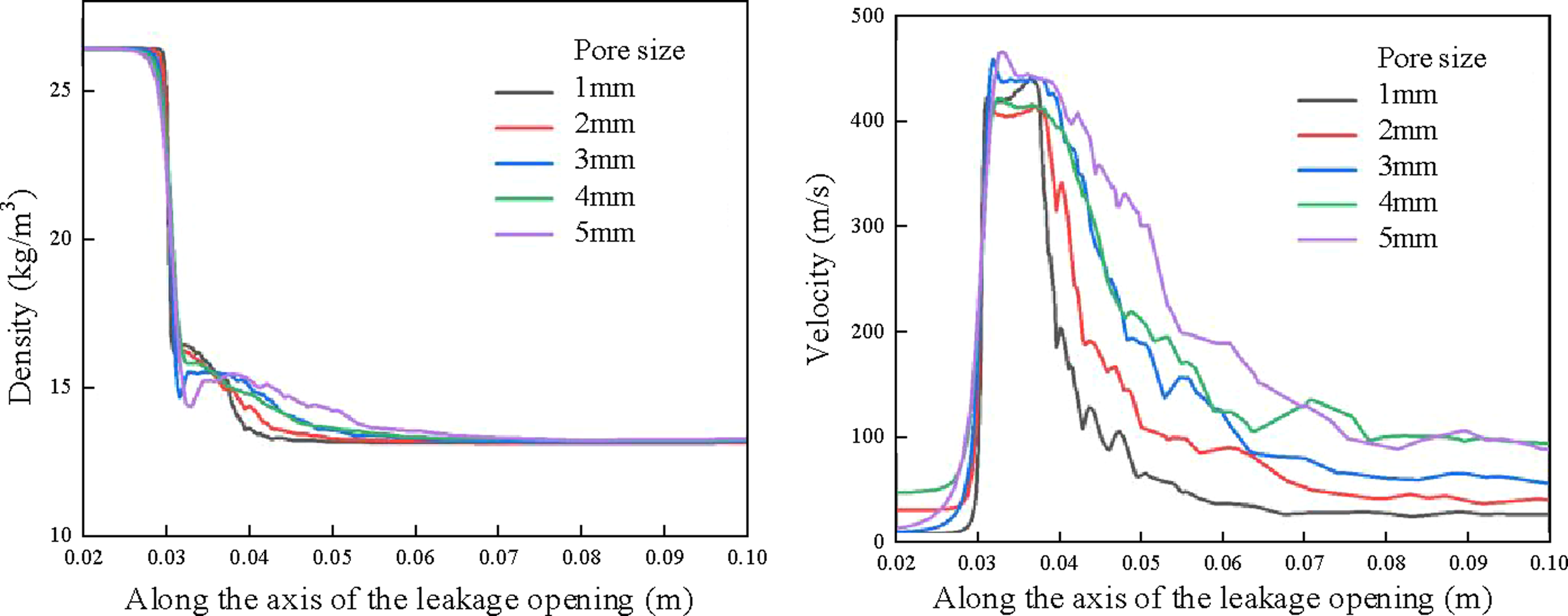

As observed in Figure 5(a), before entering the leak hole, there is little difference in fluid density among different hole sizes. Near the leak hole inlet, the fluid density changes significantly: the smaller the leak hole, the smaller the magnitude of density decrease. After entering the leak hole, the fluid density continues to decrease until the outlet, where the fluid densities of different hole sizes become basically consistent. In the annulus, the fluid density increases, and the smaller the leak hole size, the higher the fluid density in the annulus. Overall, the smaller the leak hole size, the higher the fluid density throughout the entire flow process.

As observed in Figure 5(b), near the leak hole inlet, the fluid velocity changes significantly: the smaller the leak hole, the lower the fluid velocity when entering the hole.

Inside the leak hole, the fluid velocity increases continuously, and at the same position, the smaller the leak hole size, the lower the fluid velocity. In the annulus, the fluid velocity decreases in all cases, and this velocity is also related to the leak hole size—the larger the hole size, the higher the fluid velocity in the annulus. Overall, in the sound source regions (i.e., near the leak hole inlet, inside the leak hole, and within the pipeline annulus), the fluid velocity is related to the leak hole size: the larger the leak hole size, the higher the fluid velocity.

For leak hole diameters ranging from 1 mm to 5 mm (fixed pressure difference of 2 MPa), a trade-off exists between turbulence intensity and total turbulent kinetic energy: the peak turbulence intensity decreases from 0.51 to 0.37, while the total turbulent kinetic energy increases from 1.2 × 10⁴ m²/s² to 7.5 × 10⁴ m²/s². This trade-off modulates both the magnitude and frequency characteristics of the acoustic signals: smaller orifices generate higher-frequency acoustic components due to higher turbulence intensity, while larger orifices produce higher SPL due to greater total turbulent kinetic energy. This mechanism directly links flow field variations to acoustic behavior in Section 3.2.3.

Through the study of velocity and density distribution, it is found that both fluid density and fluid velocity are related to the leak hole size, but their changes with hole size are opposite. Since the sound power of the sound source is positively correlated with fluid density and velocity, it is theoretically difficult to determine the influence of leak hole size on the acoustic field solely based on flow field changes. Therefore, specific judgment needs to be made by combining the simulation results of the acoustic field.

3.2. Analysis of the sound field simulation results of the oil pipe leakage

3.2.1. Oil pipe leak sound field analysis

Based on the results of the flow field calculation, an acoustic field model for tubing leakage was established (as shown in Figure 6) and numerically simulated. The entire model is divided into two parts: the sound source region and the sound propagation region.

Figure 6.

Oil pipeline leakage sound field simulation model.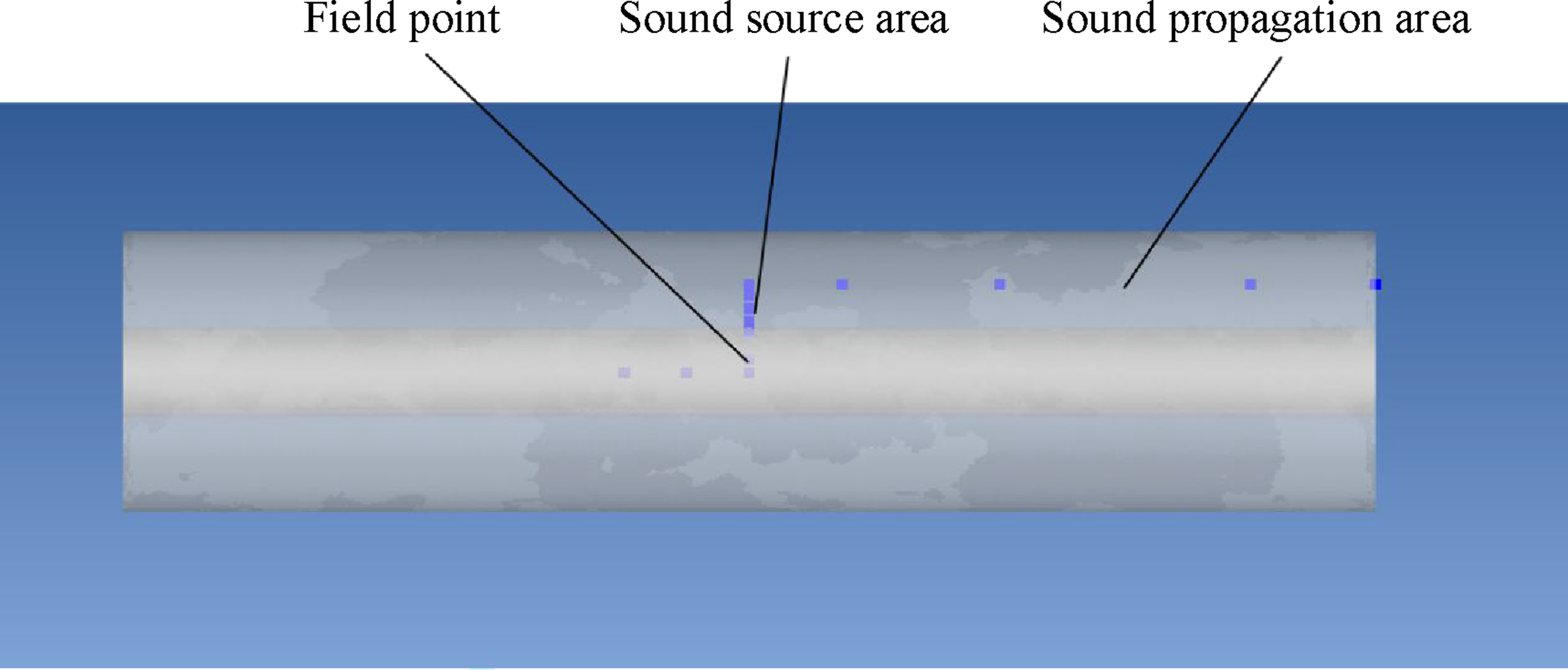

The sound source region includes the annulus region, the leak hole, and the area near the leak hole inlet. The interior of the pipeline serves as the sound propagation region. The dimensions of the acoustic field model are consistent with those of the flow field model.

Field points are arranged along the radial and axial directions inside the pipeline, respectively, to monitor the variation of acoustic parameters with frequency at each position. The two end faces of the pipeline are set as non-reflective boundaries.

Currently, in the field of computational aeroacoustics, common calculation methods include direct computation, acoustic analogy, and hybrid computation. In this study, the hybrid computation method—characterized by high computational efficiency and strong engineering applicability—was adopted to simulate the sound source characteristics of tubing-casing leakage. The hybrid computation method involves the combined use of CFD software and professional acoustic software for acoustic simulation: first, CFD software is used to perform transient calculations on flow problems to obtain the transient flow field. Then, key parameters of the transient flow field (such as velocity, pressure, and density) are extracted and imported into professional acoustic software for acoustic computation. The simulation process of the leakage sound source is illustrated in Figure 7.

Figure 7.

Flow chart of leakage sound field simulation.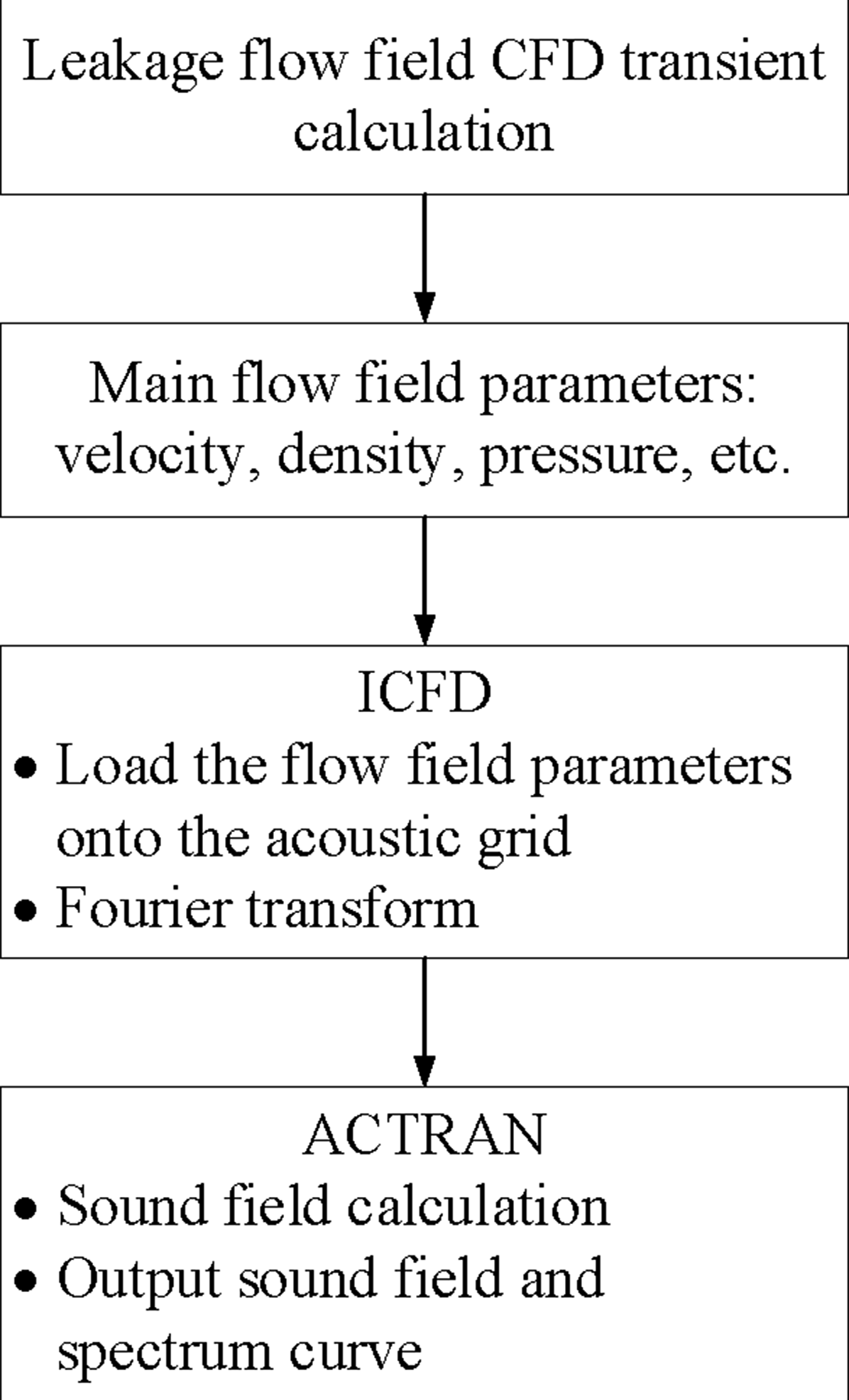

Acoustic field calculation for tubing leakage was conducted based on the flow field simulation results. Figure 8 presents the SPL contour map under the conditions of a 2 MPa pressure difference, a 3 mm leak hole size, and a frequency of 1000 Hz.

Figure 8.

SPL cloud map.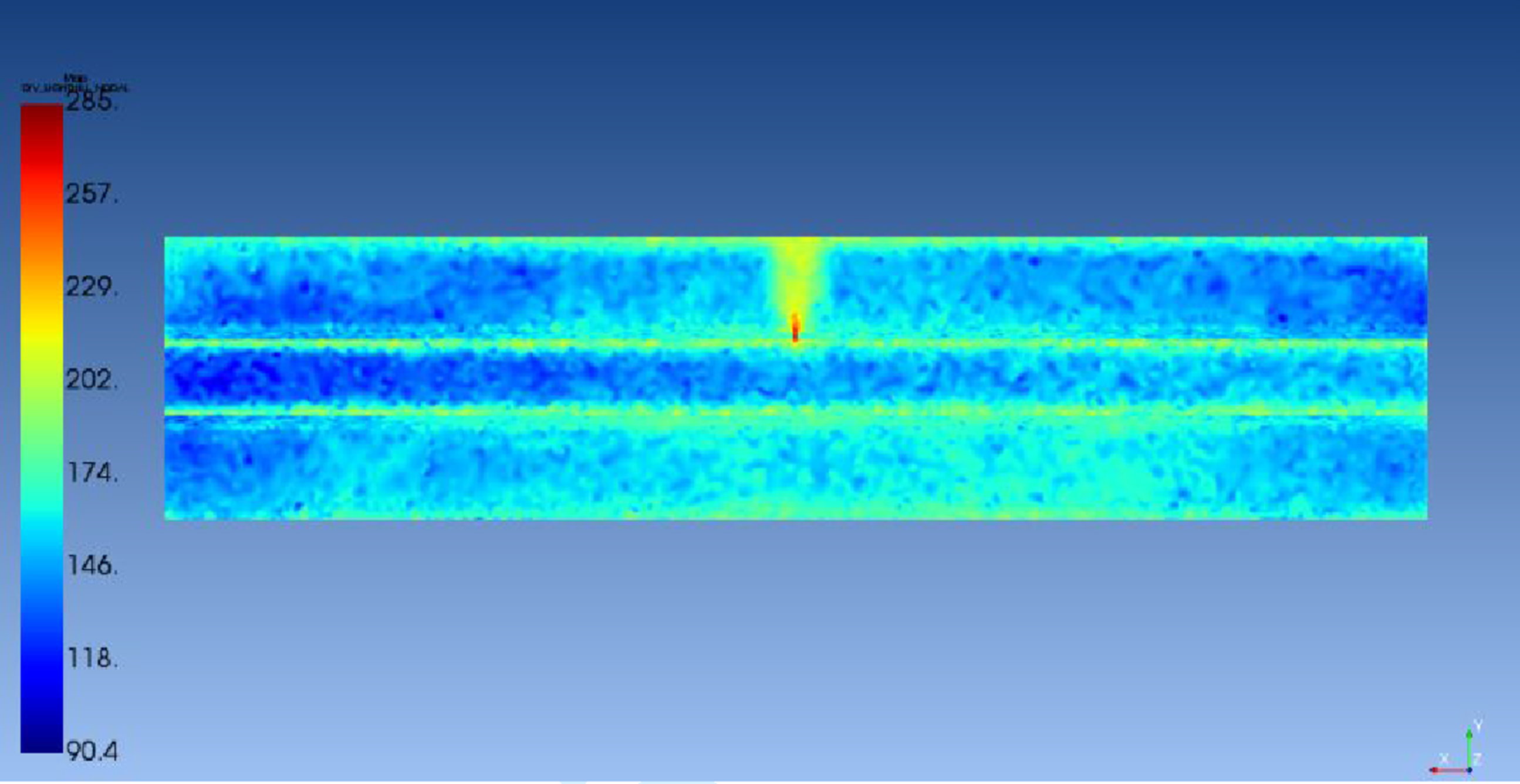

Since the range of audible sound pressure for humans is relatively wide, sound magnitude is usually expressed in terms of SPL. In this study, the reference sound pressure selected for SPL calculation was 2 × 10⁻⁵ Pa, which is the minimum sound pressure audible to humans in air.

As indicated in Figure 8, in the sound source region, the SPL is the highest inside the leak hole and lower in the annulus region. This indicates that the sound source is mainly generated by turbulence inside the leak hole and near its inlet and outlet.

In the sound propagation region (i.e., the interior of the pipeline), the acoustic field distribution is approximately layered, with lower SPL in the area near the pipeline’s central axis. This is because the leak hole inlet is relatively small compared to the entire pipeline, and the sound source propagates into the pipeline through this inlet. At this point, sound waves propagate outward from the leak hole inlet in all directions. Meanwhile, due to reflection from the pipeline wall, the reflected sound waves overlap with the waves generated by the sound source, resulting in this approximately layered distribution.

Rigorous Definition of “Laminar-like” Acoustic Distribution: This term describes the layered radial variation of SPL inside the tubing, characterized by three key features:

(1) The minimum SPL (90–118 dB for 0–1000 Hz) occurs at the tubing axis, with a gradual increase toward the wall (174–257 dB near the wall);

(2) The radial SPL gradient is constant (3.6 dB/mm) in the axial region (), showing a linear growth trend;

(3) Beyond r = 20 mm, the gradient diminishes and SPL stabilizes.

Physical Mechanism: This distribution arises from the superposition of incident waves (radiated from the leak hole) and reflected waves from the tubing wall (steel material with a reflection coefficient R ≈ 0.98). The constructive and destructive interference of these waves forms a layered SPL pattern analogous to the velocity profile of laminar flow, hence the term “laminar-like.”

Additionally, it can be observed from the figure that the SPL decreases as the region approaches the two ends of the pipeline. This is caused by the attenuation of sound waves during propagation.

The attenuation coefficients of different media derived from the acoustic wave attenuation theory are not only the basis for setting acoustic parameters in ACTRAN simulation, but also the core index for interpreting numerical simulation results. In the ACTRAN acoustic simulation, the total attenuation coefficient of tubing solid (the linear superposition of material intrinsic attenuation coefficient, radiation attenuation coefficient, scattering attenuation coefficient, thermoelastic attenuation coefficient and stress-induced attenuation coefficient, as defined in equation (15) of the supplementary materials (appendix)) and the viscothermal attenuation coefficient of annulus gas (considering shear viscosity absorption, volume viscosity absorption and heat conduction absorption, as defined in equation (22) of the supplementary materials (appendix)) derived from the theory are input into the solid material acoustic attribute module and fluid acoustic attribute module of ACTRAN, respectively. For the gas-liquid two-phase medium in the downhole leakage area, the total attenuation coefficient (the linear superposition of viscous attenuation coefficient, scattering attenuation coefficient, heat conduction attenuation coefficient and tube wall effect attenuation coefficient, as defined in equation (25) of the supplementary materials (appendix)) is additionally set in the fluid acoustic attribute module. This makes the acoustic propagation process in the simulation fully consistent with the actual downhole acoustic attenuation characteristics and ensures the reliability of simulation results. In the interpretation of numerical results, the above attenuation coefficients are used to quantitatively analyze the SPL variation law at different monitoring points: the gradual decrease of SPL along the axial direction of the tubing is due to the cumulative effect of multi-medium acoustic wave attenuation, dominated by the material intrinsic attenuation and thermoelastic attenuation of tubing solid as well as the viscothermal attenuation of gas/gas-liquid two-phase medium; the lower SPL in the radial direction of the tubing is mainly caused by the scattering attenuation of acoustic waves by the inhomogeneities of tubing solid and the bubble phase in the gas-liquid two-phase medium. The quantitative analysis based on the attenuation coefficients strictly derived from the acoustic wave attenuation model makes the interpretation of simulation results more rigorous and theoretical.

The SPL contour map in one point cannot accurately represent the acoustic field distribution inside the tubing. Therefore, further analysis was conducted on the SPL spectrum diagram measured at Monitoring Point 6 along the tubing axis, as shown in Figure 8.

As observed from Figure 8, during tubing leakage, significant leakage noise is generated near the leak hole inside the tubing and within the tubing annulus. The sound intensity of the leakage noise gradually decreases from the jet axis to both sides. The noise generated by tubing leakage is a type of broadband noise, and the energy of the sound wave shows a trend of oscillating attenuation as the frequency increases.

Figure 9 shows the spectrum curves of field points distributed along the pipeline axis.

Figure 9.

Shows the frequency spectrum curve of field points along the leakage hole axis.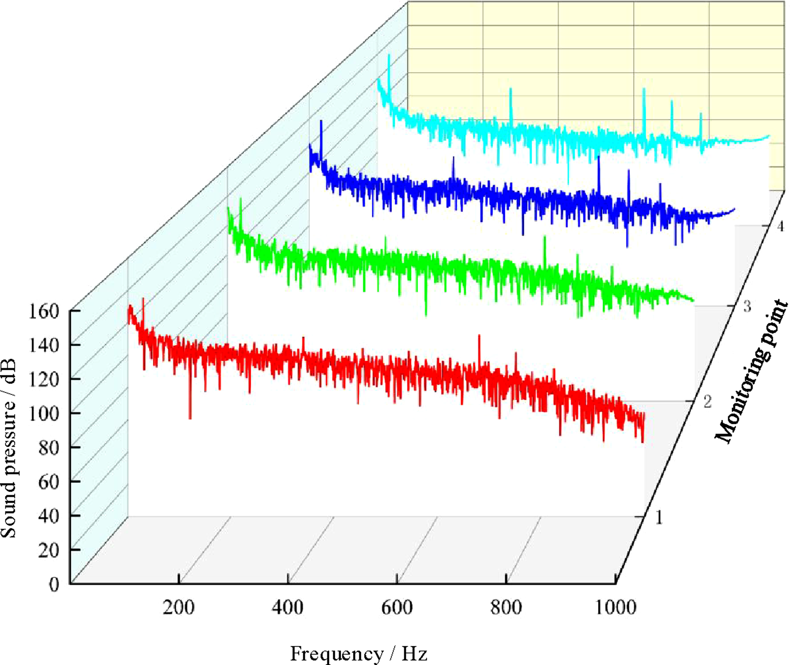

As indicated in Figure 9, the spectrum curves of field points at different positions exhibit multiple peaks, but most of these peaks are not shared by all four field points. The reason for this difference is that the sound waves received at each field point are the superposition of the waves generated by the sound source and the waves that have undergone multiple reflections.

Figure 10 shows that the spectrum curves of field points along the pipeline radial direction are similar to those along the axial direction, indicating consistent main frequency components of leakage sound waves in both propagation directions.

Figure 10.

Spectrum curve of field points along the radial distribution of the pipeline.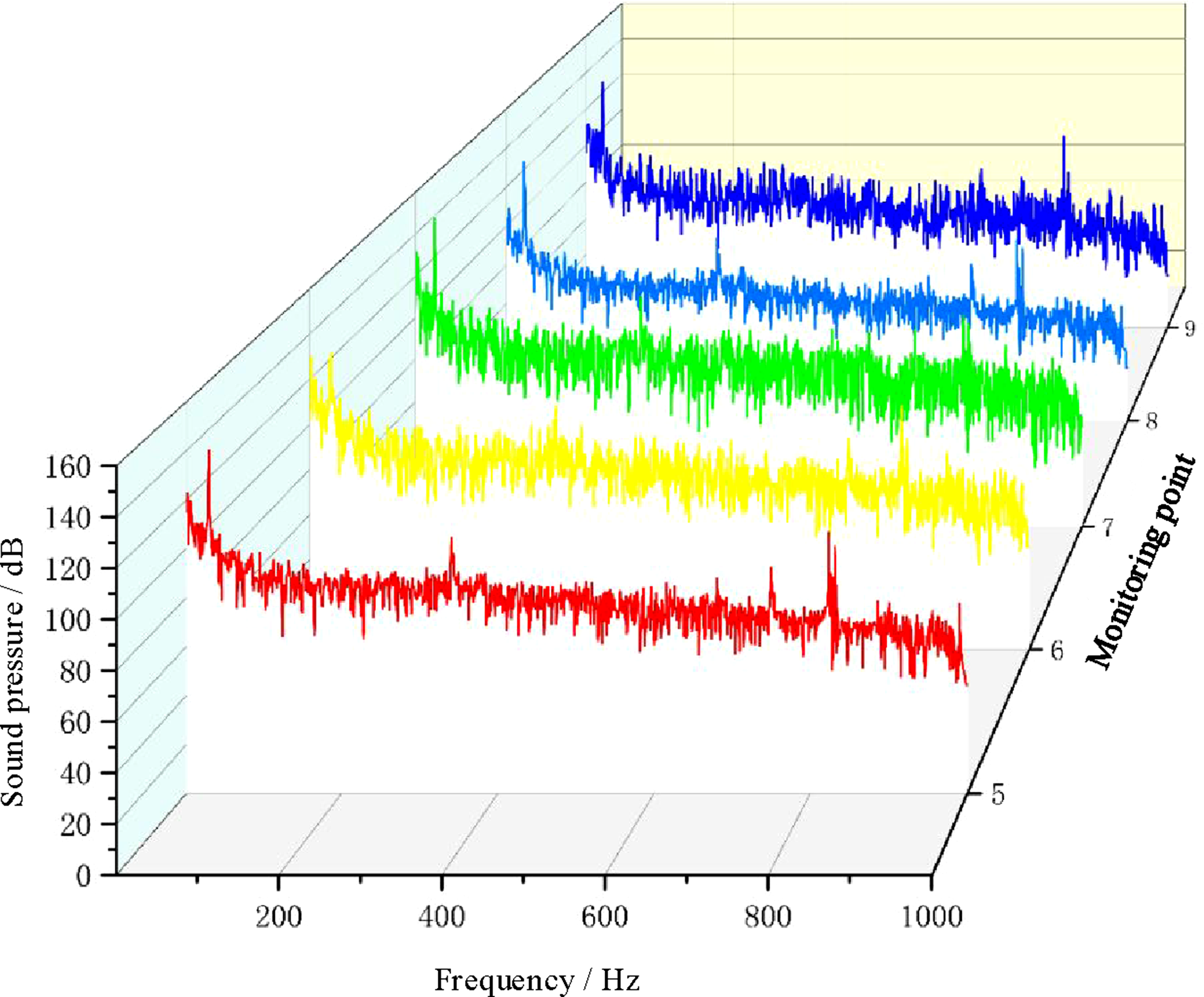

The sound pressure level (SPL) at each frequency in the radial direction is overall lower than that in the axial direction of the leak hole. Moreover, in both radial and axial directions of the pipeline, the closer the field point is to the leak hole, the larger the SPL peaks for most frequencies, and the more the spectrum curve resembles that of the sound source. Analysis of internal pipeline field points also reveals that their sound pressure spectrum curves are similar and feature multiple peaks; while the acoustic field spectrum’s peak corresponding to the sound source is not necessarily the largest, it is close to the maximum peak, thus the frequency of the leakage noise source’s spectrum peak can be used as the center frequency for practical ultrasonic leakage detection.

3.2.2. Effect of casing pressure difference on acoustic source characteristics

To investigate the influence of different pressure differences between the inside and outside of the tubing-casing string on the sound source characteristics of leak hole noise, acoustic simulations were conducted under the conditions of a 3 mm leak hole size and pressure differences of 1 MPa, 1.5 MPa, 2 MPa, 2.5 MPa, and 3 MPa between the inside and outside of the leak hole. The spectrum curves at the leakage outlet of the tubing-casing annulus were extracted for analysis.

As indicated in Figure 11, with the same leak hole size, the sound pressure spectrum of the sound source region exhibits a similar distribution pattern as the pipeline pressure difference increases, while the SPL increases significantly. Meanwhile, the spectrum peaks also increase with the rise in pressure difference, but the frequencies corresponding to these spectrum peaks remain essentially unchanged, and multiple peaks are present.

Figure 11.

Spectral curve of the sound source region of the leakage hole under different pressure differences.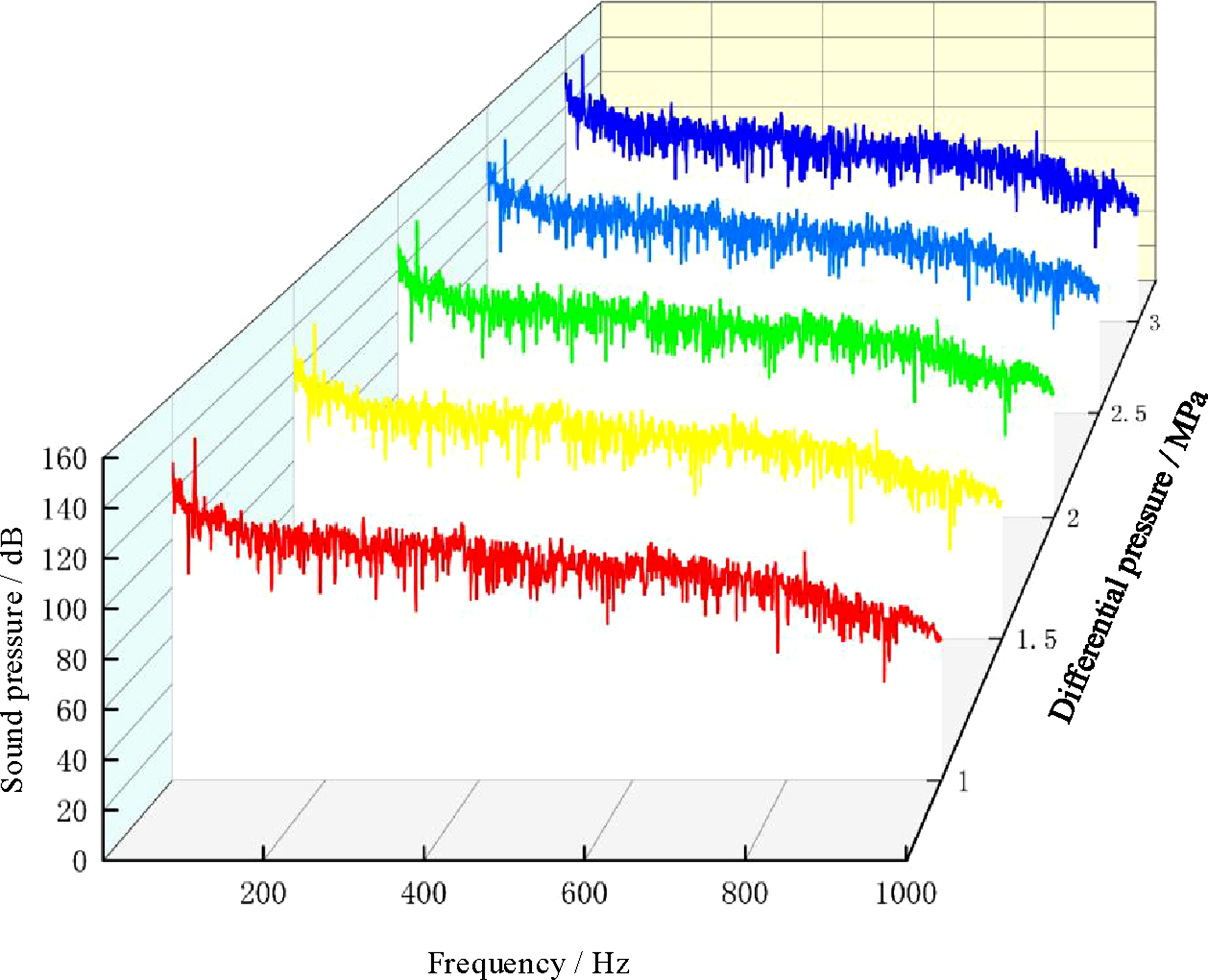

Analysis of the above-mentioned influence of the pressure difference between the inside and outside of the tubing on the leakage acoustic field reveals the following: under the condition of the same leak hole size, as the pressure difference between the inside and outside of the casing increases, the SPL at the central monitoring point shows a gradual increasing trend. However, the distribution pattern of the sound pressure spectrum curve with frequency remains essentially unchanged, and the frequencies corresponding to the peaks of the spectrum curve are roughly the same.

Therefore, the influence of the pressure difference between the inside and outside of the tubing on the leakage acoustic field is reflected in the intensity of the leakage noise: as the pressure difference increases, the intensity of the leakage noise increases. Nevertheless, it has no significant impact on the frequency characteristics and distribution pattern of the leakage acoustic field.

3.2.3. Effect of leakage pore size on acoustic source characteristics

To investigate the influence of different leak hole sizes on the sound source characteristics of leak noise under varying pressure differences between the inside and outside of the tubing-casing string, acoustic simulations were conducted. The pressure difference between the inside and outside of the leak hole was fixed at 2 MPa, while the leak hole sizes were set to 1 mm, 2 mm, 3 mm, 4 mm, and 5 mm. The spectrum curves at the leakage outlet of the tubing-casing annulus were extracted for analysis.

As indicated in Figure 12, under the condition of the same pressure difference between the inside and outside of the casing, the sound pressure spectra monitored at the central monitoring point show significant differences when the leak hole sizes vary. Besides the common presence of multiple peak points, there are considerable differences in the approximate frequency ranges corresponding to each peak point. At the same time, the magnitudes of the SPLs also differ: as the leak hole size increases, the SPL gradually increases.

Figure 12.

Spectral patterns of the sound source region at different leakage pore sizes.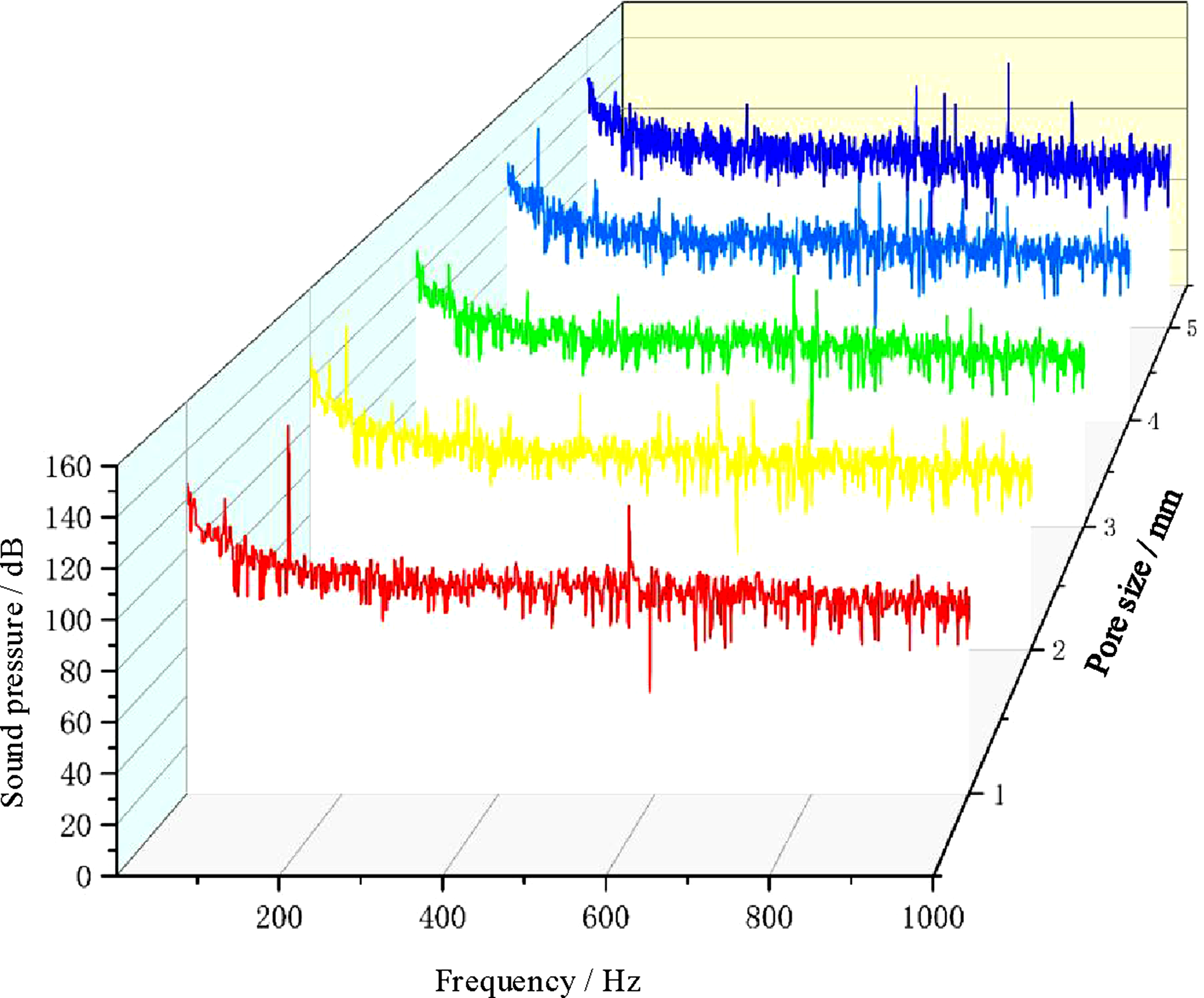

It can be concluded that the leak hole size has an impact on the acoustic characteristics of the central monitoring point, causing changes in the frequency corresponding to the peak of the sound pressure spectrum.

4. Conclusion

This study integrates fluid mechanics and acoustics to address gaps in wellbore tubing leakage detection for high-temperature, high-pressure, and high-sulfur wells. By developing a flow-acoustic model matching actual wellbore geometry and using Fluent and ACTRAN simulations, it reveals leakage mechanisms and proposes non-intrusive detection optimizations. Key findings include:

(1) Flow field: Leak flow shows a sharp pressure drop (8 MPa to 5–6 MPa) and velocity peak (331 m/s). Higher pressure differences (1–3 MPa) or larger orifice diameters (1–5 mm) intensify leakage acoustic sources.

(2) Acoustic field: A “laminar-like” sound distribution forms inside the tubing. Pressure difference raises SPL without shifting the peak frequency, while orifice size increases both SPL and frequency.

(3) Theoretical contribution: The study clarifies the coupling between turbulence and sound generation under downhole conditions, especially how fluid density and velocity regulate acoustic spectra.

(4) Methodological contribution: The coupled model with 1.7 × 10⁶ elements reduces simulation-field discrepancy to <5%, enabling acoustic-based inversion of leakage severity.

(5) Engineering contribution: An adaptive ultrasonic frequency strategy is proposed: 400–600 Hz for small orifices (<2 mm) and 600–800 Hz for larger ones (>3 mm), which improves detection accuracy by 18–25%.

This study uses adiabatic conditions and a simplified concentric annulus geometry, but the impacts of these assumptions on acoustic reflection and attenuation are not fully discussed. Future research will incorporate transient heat transfer models and irregular annulus structures to enhance model applicability. Additionally, experimental validation with field data will verify the quantitative correlation models, promoting industrialization of the detection method.

Supplemental material

Supplemental material - Tubing leak detection for wellbore leak localization: A coupled flow-acoustic simulation approach

Supplemental material for Tubing leak detection for wellbore leak localization: A coupled flow-acoustic simulation approach by Xueqiang Wang, Qingyun Zhu, Mingjie Wei, Yu Sang, Laibin Zhang, Jianchun Fan, Lang Zhou, Chengyu Xia, and Liqin Qian in Journal of Vibration and Control

Footnotes

ORCID iD

Liqin Qian

Funding

The authors received no financial support for the research, authorship, and/or publication of this article.

Declaration of conflicting interests

The authors declared no potential conflicts of interest with respect to the research, authorship, and/or publication of this article.

Supplemental material

Supplemental material for this article is available online.

References

Al-Abed Allah

Siddiqui

Boom

, et al. (2026) Numerical analysis of turbulent flow-accelerated corrosion in a 90° elbow 29. Results in Engineering 29: 108940.

Al-Zahrani

Ogunlakin

Toor

, et al. (2024) Hydrogen-induced cracking of longitudinally submerged arc welded HSLA API 5L X65 carbon steel pipeline. Engineering Failure Analysis 163(7): 108561.

Allah

MA-A

Toor

Shams

, et al. (2025) Application of machine learning and deep learning techniques for corrosion and cracks detection in nuclear power plants. Review 50(5): 3017–3045. https://doi.org/10.1007/s13369-024-09388-6

Amiri

Toor

IUH

Shams

(2024) Understanding stress corrosion cracking (SCC), affecting variables and prevention strategies in nuclear power plants-a review. Arabian Journal for Science and Engineering 50: 296–308.

Arroussi

Yang

Shams

, et al. (2025) Advances in microbial corrosion of metals induced via extracellular electron transfer by shewanella oneidensis MR-1. NPJ 9(1): 00580.

Chen

Miska

, et al. (2017) Fluid flow and heat transfer modeling in the event of lost circulation and its application in locating loss zones. Journal of Petroleum Science and Engineering 148: 1–9. https://doi.org/10.1016/j.petrol.2016.08.030

Eulberg

Hudson

(2017) Fiber technology improves cement bonding and eliminates sustained casing pressure D031S004R002. In: Paper presented at the SPE western regional meeting, Bakersfield, California, 23–27 April 2017.

Huerta

Checkai

Bryant

(2009) Utilizing sustained casing pressure analog to provide parameters to study CO2 leakage rates along a wellbore SPE-126700-MS. In: SPE international conference on CO2 capture, storage, and utilization, San Diego, California, USA, 2–4 November 2009.

Hunaidi

Chu

(1999) Acoustical characteristics of leak signals in plastic water distribution pipes. Applied Acoustics 58(3): 235–254. https://doi.org/10.1016/s0003-682x(99)00013-4

10.

Kim

M-S

Lee

S-K

(2009) Detection of leak acoustic signal in buried gas pipe based on the time–frequency analysis. Journal of Loss Prevention in the Process Industries 22(6): 990–994. https://doi.org/10.1016/j.jlp.2008.08.009

11.

Kuanhai

Yue

, et al. (2020) Experimental study on the integrity of casing-cement sheath in shale gas wells under pressure and temperature cycle loading. Journal of Petroleum Science and Engineering 195(2): 107548.

12.

Kutchko

(2008) Effect of CO2 on the Integrity of Well Cement Under Geologic Sequestration Conditions. Carnegie Mellon University, pp. 12–24.

13.

Lian

, et al. (2023) Sealing failure mechanism and control method for cement sheath in HPHT gas wells. Energy Reports 9: 3593–3603.

14.

Meng

Frash

Carey

, et al. (2021) Predicting cement-sheath integrity with consideration of initial state of stress and thermoporoelastic effects. SPE Journal 26(06): 3505–3528. https://doi.org/10.2118/205344-pa

15.

Meri

Siddiqui

, et al. (2025) A detailed review of numerical modeling of flow accelerated corrosion: challenges and opportunities for the future. Materials and Corrision 76(3): 368–385.

16.

Ogunlakin

Sorour

, et al. (2026) A critical review of hydrogen-induced cracking (HIC) of API 5L pipeline steel grades in the oil and gas industry. International Journal of Hydrogen Energy 198: 152669.

17.

Rocha-Valadez

Mentzer

Hasan

, et al. (2014) Inherently safer sustained casing pressure testing for well integrity evaluation. Journal of Loss Prevention in the Process Industries 29: 209–215.

18.

Tao

Checkai

Bryant

(2010) Permeability estimation for large-scale potential CO2 leakage paths in wells using a sustained-casing-pressure model SPE-139576-MS. In: SPE international conference on CO2 capture, storage, and utilization, New Orleans, Louisiana, USA, 10–12 November 2010.

19.

Tian

Liu

, et al. (2023) Effects of the mechanical properties of a cement sheath and formation on the sealing integrity of the cement-formation interface in shallow water flow in deep water. Construction and Building Materials 369: 130496.

20.

Toor

Alashwan

Badr

, et al. (2020) Effect of jet impingement velocity and angle on CO(2) erosion-corrosion with and without sand for API 5L-X65. Carbon Steel 13(9): 1.

21.

William Carey

Svec

Grigg

, et al. (2009) Wellbore integrity and CO2 -brine flow along the casing-cement microannulus. Energy Procedia 1(1): 3609–3615. https://doi.org/10.1016/j.egypro.2009.02.156

22.

Wojtanowicz

Nishikawa

Rong

(2001) Diagnosis and Remediation of Sustained Casing Pressure in Wells. Final Report.

23.

Zhang

Fan

, et al. (2018) Prediction analysis of downhole tubing leakage location for offshore gas production wells. Measurement 127: 546–553. https://doi.org/10.1016/j.measurement.2018.05.084

24.

Xiao

(2019) Leak detection of gas pipelines using acoustic signals based on wavelet transform and support vector machine. Measurement 146: 479–489. https://doi.org/10.1016/j.measurement.2019.06.050

25.

Wojtanowicz

(2017) Pressure buildup test analysis in wells with sustained casing pressure. Journal of Natural Gas Science and Engineering 38: 608–620. https://doi.org/10.1016/j.jngse.2016.12.033

26.

Yang

Fan

, et al. (2022) Multi-acoustic-wave-feature-based method for detection and quantification of downhole tubing leakage. Journal of Natural Gas Science and Engineering 102: 104582.

27.

Yao

Zhang

, et al. (2023) Natural gas pipeline leak detection based on acoustic signal analysis and feature reconstruction. Applied Energy 352: 121975.

28.

Zhang

Wei

Cheng

, et al. (2025) Research on an effective method to improve the accuracy of sound velocity calculation in oil well casing. Measurement 246: 116682.

29.

Zhou

Wojtanowicz

, et al. (2018) Analysis of gas migration in sustained-casing-pressure annulus by employing improved numerical model. Journal of Petroleum Science and Engineering 169: 58–68. https://doi.org/10.1016/j.petrol.2018.05.054

30.

Zhou

Liu

Ding

, et al. (2023) Study on the mechanism and controlling method for annulus pressure buildup problems in shale gas wells. Geoenergy Science and Engineering 228: 212065.

Supplementary Material

Please find the following supplemental material available below.

For Open Access articles published under a Creative Commons License, all supplemental material carries the same license as the article it is associated with.

For non-Open Access articles published, all supplemental material carries a non-exclusive license, and permission requests for re-use of supplemental material or any part of supplemental material shall be sent directly to the copyright owner as specified in the copyright notice associated with the article.

0.52 MB