Radiative transfer and flux theory

Abstract

The fundamental phenomenological equations of radiative transfer, e.g., Lambert’s cosine rule and the radiant transport equation, are derived from an analysis based on the Cauchy flux theory of continuum mechanics. For the classical case, where the radiance is distributed regularly over the unit sphere, it is shown that Lambert’s rule follows from a balance law for the transfer of radiative power in each direction u on the sphere, together with the appropriate Cauchy postulates and the additional assumption that the corresponding flux vector field j_u be parallel to u. The standard radiant transport equation follows from the additional assumption that radiant flux is given as the advection of radiant energy density. A theory is also presented for the singular limit of isolated rays, where the distribution of radiance on the sphere reduces to a Borel measure.

Keywords

Radiative transfer radiation radiometry flux stress Cauchy singular distribution

1. Introduction

We study the basic elements of radiometry from the point of view of flux and stress theory of continuum mechanics. Specifically, identifying physical space with $R^{3}$ , let x be a point on the boundary ∂R of some region R in space, let u be some unit vector and let θ denote the angle between u and the unit normal n to ∂R at x. Then, we recall that ignoring the dependence on the wavelength, the radiative energy flux,¹ the irradiance, E, out of ∂R at x is traditionally given in terms of the radiance field (radiative intensity) I(x, u) by

E = \int_{S^{2}} I (x, u) \cos θ (u) d ω (u),

(1)

where S² is the unit sphere containing all directions u and ω denotes the solid angle on the sphere. The relation

\frac{d E}{d ω} = I (x, u) \cos θ

(2)

is usually referred to as Lambert’s cosine rule (see, e.g., [1, p. 20], [2, p. 20] and [3, p. 60]). Thus, the total radiative energy flow out of R is given by

P = \int_{\partial R} [\int_{S^{2}} I (x, u) \cos θ (u) d ω (u)] d A .

(3)

We show below that these traditional relations and more general expressions for the radiative energy flux follow from the theory of Cauchy fluxes supplemented with a single additional postulate. For the case where the radiance distribution at a point is a real-valued function defined on S², Cauchy’s postulates are applied to the flux of energy in a generic direction u to yield a flux vector field j_u. Alternatively, and this is the approach used later for the more general situation where the distribution at a point may be as singular as a measure, the collection of flux vector fields, {j_u}, u ∈ S², may be viewed as an infinite-dimensional stress-like tensor field in the following sense. Given a point x and the unit normal vector n as above, the traditional stress tensor determines the three-dimensional vector of traction on ∂R at x. In analogy, the infinite-dimensional tensor corresponding to radiance determines the distribution of flux on the sphere S² at x, an element of an infinite-dimensional vector space C⁰(S²) of continuous functions on the sphere. From a different perspective, the situation is analogous to mixture theory (e.g. [4]) with constituent identified by u ∈ S².

We should also mention that a theory of radiometry can be derived from the principles of classical electromagnetism (e.g. [3, 5]), where the radiance is obtained as the average of a Poynting vector. In a complementary way, it can also be derived from the quantum-mechanical picture of a “photonic gas” [6], which bears a strong similarity to the classical kinetic theory of gases.

While works on radiation like those just cited provide some motivation for the present effort, we make but limited appeals to electromagnetic wave dynamics. Here, we assume only that the radiation flux field {j_u} is endowed with the defining property that j_u is parallel to u. As shown below, this property follows from one version of Poynting’s theorem and is consistent with a general definition of radiant energy flux. Moreover, it implies the traditional law of radiometry presented above and may have applicability to other forms of radiant energy transfer, such as acoustic or seismic waves.

Replacing the space of continuous functions C⁰(S²) by the space M(S²) of Borel measures on the sphere, enables us to consider irregular radiation distributions such as mono-directional radiation in isolated rays. Unfortunately, the property of radiation described above cannot be applied directly to irregular distributions of radiation on the sphere because j_u may not be considered as well defined. However, an analogous generalized formulation of the property is suggested by using basic notions of measure theory. We recall that the the notion of concentrated rays represents a geometric-optics model that is often adopted in classical treatments of radiant transport, even though it is strictly valid as short wavelength limit of physical or wave optics [7 –11].

2. Radiance flux fields: classical analysis

2.1. Traditional Cauchy fluxes

Traditionally, Cauchy’s flux theory (e.g. [12,13]) considers an extensive scalar property p of regions R in physical space which is represented here by $R^{3}$ . It is assumed that for each region $R \subset R^{3}$ , there is a field $ψ_{R} : \partial R \to R$ , the flux of p out of R, that represents the total flux Ψ_R of p through the boundary ∂R in the form

Ψ_{R} = \int_{\partial R} ψ_{R} d A .

(4)

A collection {ψ_R} of fields on the boundaries of all regions $R \subset R^{3}$ will be referred to as a flux system. Cauchy’s flux theory is developed on the basis of the following assumptions.

2.1.1. Boundedness (balance)

Let |R| denote the volume of the region R. It is assumed that there is a positive constant C such that

| Ψ_{R} | \leq C | R | .

(5)

The boundedness assumption above is usually motivated by a balance principle as follows. It is assumed that the total flux of the property p out of R is equal to the rate of production of the property within R minus the rate of change of the total of p in a fixed region $R \subset R^{3}$ . Thus, let ρ be the density of p in $R^{3}$ and let r be the radiant source density of p in $R^{3}$ , then

\int_{R} \partial_{t} ρ d V + \int_{\partial R} ψ_{R} d A = \int_{R} r d V .

(6)

The last balance equation, once supplemented by appropriate boundedness assumptions for ∂_tρ and r, will imply (5).

It is observed that this assumption rules out irregular sources of the property such as those concentrated on surfaces, lines, or points. This reflects the classical point of view in which such singularities are removed from the region of interest.

2.1.2. Cauchy’s postulate of locality

When one considers the dependence of the field ψ_R on the region R, the locality postulate implies that this dependence is of a very short range. Specifically, it states that for x ∈ ∂R, ψ_R(x) depends on R only through the unit normal n(x) to ∂R at x. Let S² denote the two-dimensional unit sphere in $R^{3}$ containing the collection of unit vectors. It follows that there is a function $τ : ℝ^{3} \times S^{2} \to ℝ$ such that

ψ_{R} (x) = τ (x, n (x)) .

(7)

2.1.3. Regularity

It is assumed that τ and n are smooth functions except for subsets of zero area.

We will refer to a flux system satisfying these assumptions as a Cauchy flux system.

2.1.4. Cauchy’s flux theorem

The boundedness and regularity assumptions above imply that the dependence of τ on n is linear. Since any linear function of n may be represented by an inner product with n, it follows that for a Cauchy flux system there is a vector field $T : R^{3} \to R^{3}$ such that

ψ_{R} (x) = τ (x, n (x)) = T (x) \cdot n (x) .

(8)

We refer to T as the flux vector field associated with the property p.

Consider for example the case where the property under consideration is the radiant energy so that Ψ_R is interpreted as the flow of radiant energy through the boundary out of a region R. Then, under the foregoing assumptions, Cauchy’s flux theorem implies that there is a vector field q such that the flux out of the region R is given by the analog of (8). In fact, for this case, q·n is the irradiation in the integrand of Equation (3).

2.1.5. The differential balance

Using Cauchy’s theorem in the balance (6) we have

\int_{R} \partial_{t} ρ d V + \int_{\partial R} T \cdot n d A = \int_{R} r d V .

(9)

Using Gauss’s theorem one concludes that

\begin{matrix} div T + \partial_{t} ρ = r in R, \\ T (x) \cdot n (x) = ψ_{R} (x) on \partial R . \end{matrix}

(10)

Remark 2.1. Let {ψ_R} be a flux system. Assume that there is a differentiable vector field T such that for each region R, ψ_R = T ·n, then,

Ψ_{R} = \int_{\partial R} ψ_{R} d A = \int_{\partial R} T \cdot n d A = \int_{R} div T d V .

(11)

It follows that if div T is bounded, the boundedness assumption (5) holds. This observation is a converse of Cauchy’s theorem.

For detailed, generalized and technical presentations of Cauchy’s flux theory see for example [14] and references cited therein.

2.2. Radiance systems

The space of continuous real-valued mappings defined on the sphere will be denoted by U. For a regular region R in space, a radiance field over ∂R is a mapping

I_{R} : \partial R \to U .

(12)

For x ∈ ∂R and u ∈ S², I_R(x)(u), is interpreted as the flux of radiant power at x ∈ ∂R crossing ∂R in the direction u. It should be emphasized that this interpretation is given without justification at this point to adapt the presentation to the context of radiation (see Section 2.4).

Clearly, the radiance field may be regarded as a function ${I^{'}}_{R} : \partial R \times S^{2} \to ℝ$ by $I'_{R}$ (x, u) = I_R(x)(u). We prefer the function I_R, anticipating its generalization in Section 3.

For a given u ∈ S², the radiance field at the directionu is the function

I_{R, u} : ℝ^{3} \to ℝ, I_{R, u} (x) = I_{R} (x) (u) .

(13)

The total emitted power flux at x, the irradiance or radiant emittance is therefore given by

ψ_{R} (x) = \int_{S^{2}} I_{R} (x) (u) d ω (u) = \int_{S^{2}} I_{R, u} (x) d ω (u),

(14)

where ω is the solid angle measure. The total power transmitted through ∂R is

\begin{matrix} P_{R} = \int_{\partial R} ψ_{R} (x) d A & = \int_{\partial R} (\int_{S^{2}} I_{R} (x) (u) d ω (u)) d A . \end{matrix}

(15)

Fubini’s theorem implies that we can write

P_{R} = \int_{S^{2}} (\int_{\partial R} I_{R} (x) (u) d A (x)) d ω = \int_{S^{2}} P_{R, u} d ω (u),

(16)

where

P_{R, u} = \int_{\partial R} I_{R} (x) (u) d A (x) = \int_{\partial R} I_{R, u} (x) d A (x)

(17)

is the total power transmitted from R in the direction u ∈ S² (directional emissive power in [15]). It is noted that for a fixed u ∈ S², P_R,u is the total flow given by the flux I_R,u(x) = I_R(x)(u) on ∂R.

A radiance system is a collection {I_R} for all regions $R \subset R^{3}$ . In keeping with the flux-theoretic approach we study the dependence of the radiance I_R on the region R.

We will say that a radiance system {I_R} is a Cauchy radiance system if for each u ∈ S², the scalar-valued flux system {I_R,u} satisfies Cauchy’s postulates. From Cauchy’s theorem for scalar fluxes, it follows that for a Cauchy radiance system, for every u ∈ S², there is a vector field, the radiance vector field for the directionu,

j_{u} : R^{3} \to R^{3}, such that j_{u} (x) \cdot n (x) = I_{R, u} (x),

(18)

where n(x) is the unit normal to ∂R at x.

Using the radiance vector field, Equation (17) may be written as

P_{R, u} = \int_{\partial R} j_{u} \cdot n d A .

(19)

The existence of the radiance vector field for the direction u enables one to define the field j over $R^{3} \times R^{3}$ , whose value is a function over the sphere by

j (n, x) (u) = j_{u} (x) \cdot n .

(20)

To emphasize that $j (\cdot, x) : R^{3} \to U$ is a linear map, we will refer to $j : R^{3} \times R^{3} \to U$ as a radiation density tensor. The associated expression for the power becomes

\begin{array}{l} P_{R} = \int_{\partial R} [\int_{S^{2}} (j_{u} (x) \cdot n (x)) d ω (u)] d A, \\ = \int_{\partial R} [\int_{S^{2}} j (n (x), x) (u) d ω (u)] d A . \end{array}

(21)

As j is linear in n and using e_k to denote the kth standard base vector in $R^{3}$ , one may define

j_{k} (x) = j (e_{k}, x),

(22)

so that

j (n, x) = \sum_{k} j_{k} (x) n_{k},

(23)

and

\begin{array}{l} P_{R} = \int_{\partial R} [\int_{S^{2}} (\sum_{k} j_{k} (x) n_{k}) (u) d ω (u)] d A, \\ = \int_{\partial R} \sum_{k} n_{k} [\int_{S^{2}} (j_{k} (x)) (u) d ω (u)] d A, \\ = \int_{\partial R} \sum_{k} n_{k} q_{k} d A, \end{array}

(24)

where

q_{k} = \int_{S^{2}} (j_{k} (x)) (u) d ω (u)

(25)

are the components of the total radiant energy flux vector field q.

Remark 2.2. It is noted that the locality assumption, (7) and the resulting Cauchy formulas (8) and (18), make it possible to obtain the total flux across surfaces that are not necessarily the boundaries of regions. This holds for radiation as a particular case of flux and stress theory. Thus, let S be a surface oriented by a choice of sense of the unit normal n. Then, j_u(x) ·n(x) will give the flux for the direction u through the surface at x. The flux will be considered positive if it agrees with the sense chosen for n and will be equal to the flux across the boundary of every region R containing x on its boundary provided that n is the outward pointing normal to R. To compute the total flux through S for the direction u, one has to replace the integration over ∂R by integration over S. (It is noted that at this point, u serves merely as a parameter and its direction has no relation to the direction of the flux vector j_u.)

2.3. The source term and differential balance equation

Using Gauss’s theorem in Equation (19) one has

P_{R, u} = \int_{R} div j_{u} d V

(26)

and

\begin{matrix} P_{R} & = \int_{S^{2}} [\int_{R} div j_{u} d V] d ω, \\ = \int_{R} [\int_{S^{2}} div j_{u} d ω] d V . \end{matrix}

(27)

A balance equation for the energy flux in the direction u ∈ S² will be of the form

\int_{R} \partial_{t} ρ_{u} d V + \int_{\partial R} I_{R, u} d A = \int_{R} r_{u} d V

(28)

and with Equation (18)

\int_{R} \partial_{t} ρ_{u} d V + \int_{\partial R} j_{u} \cdot n d A = \int_{R} r_{u} d V .

(29)

The corresponding differential balance equation is

div j_{u} + \partial_{t} ρ_{u} = r_{u},

(30)

which may be regarded as a balance equations for “rays” in the particular direction u. Integration over the unit sphere will then give the balance for total energy of all rays.

2.4. The basic assumptions for radiance

It is noted that thus far only a few properties of radiation have been considered. For example, one could replace the sphere S² by some other space B so that the space U would be the collection of continuous functions on B. For example, if the space B is the set {1, 2, 3}, the space U of real-valued functions on it is identical to $R^{3}$ by identifying w_i with w(i) for each i ∈ B = {1, 2, 3}. Clearly, continuity is not relevant in this example. Such a construction will lead us to traditional stress theory as we remark below. In fact, if we do not insist that the functions considered be real-valued, then the set U can be any set. We could consider a system {I_R,u}, for each region R and each u ∈ B and require that it satisfies Cauchy’s postulates for any fixed u. For each u ∈ B, Cauchy’s theorem would imply the existence of a flux vector field j_u.

As anticipated above, for the special case of radiation we take

j_{u} = j_{u} u,

(31)

where j_u = |j_u| is a positive real-valued function on $R^{3}$ . It follows from Equation (18) that

I (x, n, u) = j_{u} (x) u \cdot n .

(32)

Denoting by θ the angle between the vectors u and n,

I (x, n, u) = j_{u} (x) \cos θ .

(33)

With this basic assumption, the interpretation of I_R(x)(u) as the flux of energy flowing in the direction u is justified. Since j_u is positive for vectors u that point out of R, the power I_R(x)(u) = j_u(x)u·n, flows out of R, and for vectors u that point into R, I_R(x)(u) is the incoming power. It is observed that we put no restriction on the dependence of j_u on u so that I_R(x)(u) and I_R(x)(−u) are independent and represent illumination from opposite directions. As in Remark 2.2, one can also consider surfaces that need not be the boundaries of regions so that “incoming” and “outgoing” are interpreted in accordance with the chosen orientation.

Equation (19) may now be written as

P_{R, u} = \int_{\partial R} j_{u} u \cdot n d A .

(34)

Thus, the expression (21) for the power becomes

\begin{array}{l} P_{R} = \int_{\partial R} [\int_{S^{2}} j_{u} (x) \cos θ (u) d ω (u)] d A, \\ = \int_{\partial R} [\int_{S^{2}} j_{u} (x) u d ω (u)] \cdot n (x) d A, \end{array}

(35)

so that the radiant energy flux vector field is given by

q (x) = \int_{S^{2}} j_{u} (x) u d ω (u),

(36)

which represents one member of the hierarchy of moments of j_u that are relevant to illumination theory, as discussed in [16].

Alternatively, we may write

\begin{matrix} P_{R} & = \int_{S^{2}} [\int_{\partial R} j_{u} (x) n d A] \cdot u d ω (u), \\ = \int_{S^{2}} s_{u} \cdot u d ω, \end{matrix}

(37)

where

s_{u} = \int_{\partial R} j_{u} (x) n d A

(38)

represents the total contribution of the radiation in the direction of u crossing ∂R (cf. radiant intensity $I$ in [9, Equation (2.1.9)]).

Comparing Equation (35) with traditional expositions of radiation theory (e.g. [7 –11]), it is noted that j_u(x) is the specific intensity (e.g. [7 –9]) or radiative intensity (e.g. denoted by I(x, u) in [10] and by K in [7]).

Remark 2.3. To provide some insight on the various objects introduced here, we compare the notions under consideration to stress theory of continuum mechanics. In continuum mechanics, the traction vector t, determined by its three components t_i, depends on the point x and external unit normal n. Thus, in analogy with the three components t_i, the radiation field is determined by the infinite number of “components”I_R,u(x) = I_R(x)(u) parametrized by the direction u. As an alternative analogy, one may appeal to the continuum theory of mixtures [4], with a continuous distribution of components indexed by u.

The radiant flux j_u is thus analogous to the material traction t_u in a given direction u given in terms of the mechanical stress tensor T by

t_{u} = T (u) = T^{T} u

(39)

Pursuing this analogy further, we recall that the mechanical energy flux in space given in terms of (barycentric) material velocity v by

j_{E} = ρ_{E} v + q - T^{T} v, where ρ_{E} = ρ_{0} (v^{2} / 2 + ε),

(40)

where ρ₀ is mass density, $ϵ$ specific internal energy and q is heat flux. Whenever q = 0 and T = −pI is isotropic, we obtain the result that j_E is parallel to the material velocity v.

According to one convention, [17] and [18, Section 4.2], the analogous formula for (Poynting) electromagnetic energy flux in an isotropic linear medium with constant optical properties is given in terms of the corresponding Maxwell stress T_e and energy density ρ_e by

\begin{matrix} j_{e} = S = - T_{e}^{T} v, where T_{e} = T_{e}^{T} = D \otimes E + B \otimes H - ρ_{e} I, \\ ρ_{e} = \frac{1}{2} (D \cdot E + B \cdot H), and S = D \times H \end{matrix}

(41)

where the notation for electromagnetic fields is standard. Hence, the relevant velocity is given in terms the Poynting vector S by v = S/ρ_e, since the deviator of T_e does not contribute to energy flux. Therefore, if we identify a unit vector u = v/|v| = S/|S|, we may identify j_e with the radiant flux j_u of interest here. More generally, the postulated parallelism of j_u and u serves to define rays in terms of energy flux.

We may now apply Green’s theorem to Equation (38) to obtain

s_{u} = \int_{R} \nabla j_{u} d V .

(42)

Thus, the total flux out of R may be expressed as

\begin{matrix} P_{R} = \int_{S^{2}} [\int_{R} \nabla j_{u} d V] \cdot u d ω, \\ = \int_{R} [\int_{S^{2}} \nabla j_{u} \cdot u d ω] d V . \end{matrix}

(43)

which represents the directional derivative of j_u in the direction of u, often expressed in the form

u \cdot \nabla j_{u} = \partial_{s} j_{u} : = \frac{\partial j_{u}}{\partial s}

(44)

(see [10]), with ds referring to incremental ray trajectory. Evidently, the same result could be obtained by applying Green’s theorem to the second line of Equation (35). The differential balance equation for the radiation in the direction u, Equation (30), assumes the form

\partial_{t} ρ_{u} + u \cdot \nabla j_{u} = r_{u} .

(45)

Remark 2.4. Assume that ∂_tρ_u = r_u = 0 in the last equation. If follows that the above directional derivative vanishes:

u \cdot \nabla j_{u} = 0,

(46)

This result, regarded as the conservation of j_u under translation in the direction u, is sometimes referred to as the “fundamental theorem of radiometry” (e.g. [19, pp. 18–19]), which is obviously restricted to steady states of transparent media.

In line with the preceding considerations of electromagnetic energy flux we can take

j_{u} = c_{u} ρ_{u} and j_{u} = v ρ_{u}, where v = c_{u} u,

(47)

where c_u represents the photocentric speed, with dependence on u allowing for the possibility of an anisotropic medium. In the oft-studied case of isotropic media with c_u = c, independent of u and x, Equation (45) can be written in the alternative forms

\begin{matrix} {\overset{\cdot}{ρ}}_{u} : = \partial_{t} ρ_{u} + v \cdot \nabla ρ_{u} = r_{u} \\ and \\ j'_{u} : = \frac{1}{c} \partial_{t} j_{u} + \partial_{s} j_{u} = r'_{u}, where r'_{u} = r_{u} / c . \end{matrix}

(48)

While the first form represents a standard balance equation, the second form is the most common to the radiation literature, where the term ∂_tj_u is often neglected and the nominal source term $r'_{u}$ represents lineal emission, absorption and scattering along a given direction u.

We note that the first member of (48) can be cast into the general form (30) which covers the case of an inhomogeneous, refractive medium with variable speed c_u = c_u(x). From the preceding relations, it is an easy matter to derive the total radiant energy balance:

\partial_{t} ρ + div q = r,

(49)

where q is the total radiant energy flux in (25) which, to little advantage, can also be expressed as

q = \bar{v} ρ, where \bar{v} = \frac{1}{ρ} \int_{S^{2}} c_{u} ρ_{u} u d ω

(50)

The nominal source term r in (50) is usually assumed to describe the interaction of radiation and matter, the latter representing the so-called “participating medium” [10] in the literature on radiant heat transfer. The same “radiation” term r crops up (as −r) in the energy and entropy balances of countless works on continuum thermomechanics, as exemplified by [20] dealing with the absorption of microwave radiation. In a more general setting, it may be viewed as an essential coupling between the dynamics of radiation and matter. It is usually viewed as a dissipative heat exchange, to be distinguished from the non-dissipative coupling represented by the dependence of c_u on u and x.

In line with certain remarks in the Introduction, we further note that balance equations for radiation bear a strong resemblance to the Boltzmann equation of classical kinetic theory, with ρ_u, r_u representing, respectively, the (“singlet”) velocity distribution and the changes due to collision dynamics. However, in the case of radiant energy, the speed c_u is assumed fixed by the medium whereas the distribution of directions u is governed by r_u and possibly by interactions with a remote boundary ∂R. In this respect, we may consider radiometry to be a sort of kinetic-theory precursor to the continuum balances that one obtains by integration over u. As with classical kinetic theory, one can identify a regime of “rarefied” dynamics for transparent or “non-participating” media [10], where transport is governed by interaction with boundaries, and a regime of “collisional” dynamics, dominated by strong scattering. As mentioned below, this leads to a regime in which the advective flux vρ_u is dominated by a diffusive flux.

Remark 2.5. From Remark 2.1, it follows that if one starts from the standard expression (35), then the Cauchy postulates follow for differentiable fields j_u. In other words, the Cauchy postulates are both necessary and sufficient for that expression. Not merely some, but all differentiable radiance fields represent Cauchy radiance systems. Specifically, it follows from Equation (34) that

P_{R, u} = \int_{R} div (j_{u} u) d V

(51)

and, hence, the boundedness expression for P_R,u :

| P_{R, u} | \leq max_{x \in R^{3}} | div (j_{u} u) (x) | | R | .

(52)

2.5. Virtual power

Let u be a fixed direction is space and let $w_{u} : \partial R \to R$ be a field. One may consider the action

P_{R, u} (w_{u}) = \int_{\partial R} I_{R, u} (x) w_{u} (x) d A (x) .

(53)

We interpret P_R,u(w_u) as follows. Let $W_{u} : \partial R \to R^{+}$ be a differentiable function that we interpret as a continuous array of radiation meters over the boundary that measure the radiance in the direction u with W_u(x) representing the areal density of meters at x. The field w_u is conceived as a variation of W_u. Thus, while W_u(x) should be positive by our interpretation, this limitation does not apply to w_u(x). Hence, P_R,u(w_u) is interpreted as the change of the total power of radiation propagating in the direction u measured by the distribution of meters under the variation w_u of the distribution. For short, we will refer to P_R,u(w_u) as the virtual power.

Using the radiance vector field j_u we may write the virtual power as

P_{R, u} (w_{u}) = \int_{\partial R} w_{u} (x) j_{u} (x) \cdot n (x) d A (x) .

(54)

The last equation may be transformed using Gauss’s theorem into

\begin{matrix} P_{R, u} (w_{u}) & = \int_{R} div (w_{u} j_{u}) d V, \\ = \int_{R} j_{u} \cdot \nabla w_{u} d V + \int_{R} w_{u} div j_{u} d V, \end{matrix}

(55)

and with Equation (30) we obtain

\int_{\partial R} I_{R, u} w_{u} d A + \int_{R} w_{u} (\partial_{t} ρ_{u} - s_{u}) d V = \int_{R} j_{u} \cdot \nabla w_{u} d V .

(56)

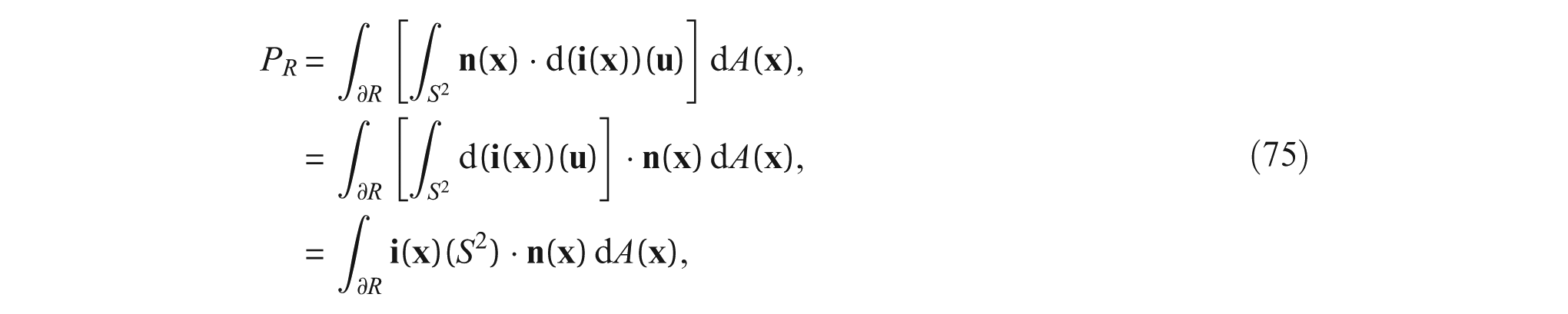
Using the basic assumption for radiance (31) we finally arrive at

\int_{\partial R} I_{R, u} w_{u} d A + \int_{R} w_{u} (\partial_{t} ρ_{u} - s_{u}) d V = \int_{R} j_{u} u \cdot \nabla w_{u} d V,

(57)

where u·∇w_u represents a directional derivative like that in (44).

3. Measure-valued radiance

3.1. Preliminaries

In the foregoing analysis, the flux of radiant energy is distributed continuously on the sphere S². For example, for a point x ∈ ∂R, a function $I_{x} = I_{R} (x) : S^{2} \to R$ describes the distribution of radiation power, where for u ∈ S², I_x(u) was interpreted as the radiation in the direction of u. It is noted that if one wishes to consider power concentrated in one particular direction u₀, a distribution such as I_x above is not sufficiently general. Now, one has to include mathematical objects such as the Dirac delta distribution, $δ_{u_{0}}$ .

It is observed that traditional treatments (e.g. [1, 10, 21]) assume explicitly that the derivative dE/dω as in Equation (2) exists and use it to define the radiative intensity. It is therefore our objective in this section to provide a setting for radiance theory in which the existence of

lim_{Δ ω \to 0} \frac{Δ E}{Δ ω}

is not required and singular distributions, such as the Dirac delta distribution, are admissible.

Thus, it is assumed henceforth that the distribution of radiation, or the radiance, at x ∈ ∂R, is generally a Borel measure on the unit sphere. Hence, if we denote the radiance at x by J_x, for any Borel subset D of the sphere S², J_x(D) denotes the measure of D indicating the total power transmitted through the pencil at x subtended by D. In particular, the irradiance is given by

E = J_{x} (S^{2}) = \int_{S^{2}} d J_{x} .

(58)

We henceforth denote by J, i the respective measures associated with I, j, reversing the alphabetical order to emphasize the distinction. In the traditional continuous case, the measure J_x is absolutely continuous relative to the solid angle measure, or area measure on the unit sphere, so that there is a Radon–Nikodym derivative

I_{x} = \frac{d J_{x}}{d ω}, I_{x} : S^{2} \to R

(59)

and

J_{x} (D) = \int_{D} I_{x} d ω .

(60)

(see [1, 21]). We will denote by M the vector space of Borel measures on the unit sphere, and so J_x ∈ M (as a generalization of I_x ∈ U). The vector space operations are naturally defined in M by (aJ_x + a′J′_x)(D) = aJ_x(D) + a′J′_x(D).

It is recalled that the space of Borel measures M may be identified with the dual space U* of the space U of continuous real-valued mappings on the sphere. Specifically, the measure J_x may be regarded as a continuous linear functional $J'_{x} : U \to R$ such that

J'_{x} (υ) = \int_{S^{2}} υ (u) d J_{x} (u), for all v \in U .

(61)

The expression above is interpreted as the virtual power flux at x for the change in a hypothetical distribution of radiance meters υ at x. In the sequel, a measure is not distinguished notationally from the linear functional it induces. In terms of this action, a natural norm on M may be defined by

| | J_{x} | | = sup_{υ \in U} \frac{J_{x} (υ)}{| | υ | |},

(62)

where $‖ υ ‖ = max_{u \in S^{2}} | υ (u) |$ . With this norm, M is provided with the structure of a Banach space.

3.2. Measure-valued densities and fluxes

In analogy with the definition of the radiance field over ∂R in (12), the basic assumption is that for every region $R \subset R^{3}$ there is a smooth function, the measure-valued radiance,

J_{R} : \partial R \to M .

(63)

The collection {J_R}, for all regions R is a measure-valued radiance system. For a given measure-valued radiance system and an element υ ∈ U, let { $J_{R, υ}$ } be the flux system such that

J_{R, υ} (x) = J_{R} (x) (υ) = \int_{S^{2}} υ d (J_{R} (x)),

(64)

i.e. the action of J_R(x) on υ is the action of a continuous linear functional on a continuous function defined on the sphere. Similarly, one can evaluate the integral of the measure J_R(x) over any integrable Borel subset $D \subset S^{2}$ to yield

J_{R} (x) (D) = \int_{D} d (J_{R} (x)) .

(65)

In analogy with Section 2.2 we now assume that for each fixed υ ∈ U, the measure-valued radiance systems {J_R,υ} satisfies Cauchy’s postulates. Let υ ∈ U be a fixed distribution. It follows from Cauchy’s theorem for scalar-valued flux systems that there is a vector field $i_{υ} = \sum_{k} i_{υ k} e_{k} : R^{3} \to R^{3}$ such that

J_{R, υ} (x) = J_{R} (x) (υ) = i_{υ} (x) \cdot n (x) = \sum_{k} i_{υ k} (x) n_{k} (x)

(66)

for any x ∈ ∂R. It follows from Equation (66) that i_υ and i_{υ
k} depend on υ ∈ U continuously and linearly. As i_{υ
k}(x) is real, there are three elements i_k(x) ∈ M such that i_{υ
k}(x) = i_k(x)(υ). Hence,

J_{R, υ} (x) = \sum_{k} n_{k} (x) i_{k} (x) (υ) = \sum_{k} n_{k} (x) \int_{S^{2}} υ d (i_{k} (x)) .

(67)

Clearly, i_k(x) ∈ M are the three flux distributions at x corresponding to the area elements which are perpendicular to the standard base vectors in $R^{3}$ .

Using the notation $L (R^{3}, M)$ for the space of linear mappings $R^{3} \to M$ (which are also continuous as they are defined on a finite dimensional space), one can now define the mapping

i : R^{3} \to L (R^{3}, M) ≅ M \otimes R^{3}

(68)

(i (x) (n)) (υ) = i_{υ} (x) \cdot n = \sum_{k} n_{k} (x) i_{k} (x) (υ) .

(69)

Observe that for any $n \in R^{3}$ ,

\begin{matrix} \sum_{k} i_{k} (x) n_{k} & = i (x) (n), \\ = i (x) (\sum_{k} n_{i} e_{i}), \\ = \sum_{k} n_{k} i (x) (e_{k}), \end{matrix}

(70)

so that i_k(x) = i(x)(e_k) ∈ M. Thus, we may introduce the notation

i = \sum_{k} i_{k} \otimes e_{k},

(71)

and write

J_{R} = i \cdot n = (\sum_{k} i_{k} \otimes e_{k}) \cdot (n_{k} e_{k}) = \sum_{k} i_{k} n_{k} = i (n) .

(72)

The infinite-dimensional tensor i will be referred to as the measure-valued radiance tensor. In particular, for any Borel integrable set D,

\begin{matrix} J_{R} (x) (D) & = \sum_{k} i_{k} (x) (D) n_{k} (x) = i (x) (D) \cdot n (x), \\ = \sum_{k} n_{k} (x) \int_{D} d (i_{k} (x)) . \end{matrix}

(73)

In the case where the measures i(x) may be represented by densities relative to the solid angle measure ω on the sphere, one has

d i (x) = j (n, x) d ω

(74)

where j(n,x) is the radiance tensor.

Using the measure-valued radiance tensor, the total energy flux out of a region R is given as

\begin{matrix} P_{R} & = \int_{\partial R} [\int_{S^{2}} n (x) \cdot d (i (x)) (u)] d A (x), \\ = \int_{\partial R} [\int_{S^{2}} d (i (x)) (u)] \cdot n (x) d A (x), \\ = \int_{\partial R} i (x) (S^{2}) \cdot n (x) d A (x), \end{matrix}

(75)

where,

i (x) (S^{2}) = \sum_{k} i_{k} (x) (S^{2}) \otimes e_{k}

(76)

and i_k(x)(S²), k = 1, 2, 3, represent the total measures of the sphere. The energy flux vector field q is therefore given by

q (x) = \int_{S^{2}} d (i (x)) (u) = i (x) (S^{2}) .

(77)

3.3. Measure-valued radiance tensors: global approach

We present below an alternative derivation of the measure-valued radiance tensor in terms of a global radiation distribution on a region R. In order to formulate the theory, one needs integration and differentiation of functions defined on $R^{3}$ and having values in a Banach space: the space M in our case. (See for example [22, Chap. V] or [23, Chap. VIII] for details on the calculus of functions with values in Banach spaces.)

3.3.1 The analogs of Cauchy’s postulates

As in the definition of the radiance field over ∂R in (63), the basic assumption is that for every region $R \subset R^{3}$ there is a smooth function, the measure-valued radiance, J_R: ∂R→M. The total of the radiation corresponding to the region R is defined as the distribution

Φ_{R} = \int_{\partial R} J_{R} d A \in M,

(78)

where we integrate the measure J_R(x) over ∂R. In other words, for each measurable subset D_{S
²}, Φ_R(D) is the total flux of energy flowing in the directions included in the pencils determined by D from all points in ∂R.

In case Φ_R is absolutely continuous relative to the solid angle measure on the sphere, the directional emissive power P_R,u is given by the Radon–Nikodym derivative

P_{R, u} = \frac{d Φ_{R}}{d ω} (u) .

(79)

The following assumptions are made in analogy with Section 2.1.

3.3.2 Locality

It is assumed that for a point x ∈ ∂R, J_R(x) depends on R through the outwards pointing normal n(x) to ∂R at x.

It follows that there is a function

J : R^{3} \times S^{2} \to M,

(80)

to which we will refer as the Cauchy mapping, such that

J (x, n (x)) = J_{R} (x)

(81)

for any region R such that x ∈ ∂R and n(x) is the outwards pointing normal to R at x.

Using the Cauchy mapping we may rewrite the total as

Φ_{R} = \int_{\partial R} J (x, n (x)) d A .

(82)

3.3.3. Boundedness (balance)

We assume that there is a positive number C such that

| | Φ_{R} | | \leq C | R |,

(83)

where ||Φ_R|| is the norm in M of the total.

3.3.4. Regularity

It is assumed that the Cauchy mapping J is smooth.

3.3.5 The analog of Cauchy’s theorem

We outline a sketch of the proof of Cauchy’s theorem for the current settings. Consider an infinitesimal tetrahedron containing the point $x \in R^{3}$ such that for α = 0, 1, 2, 3, A_α are the areas of the faces of the tetrahedron and n_α are the unit normals to the faces. Thus, Equation (82) assumes the form

Φ_{R} = \sum_{α} J (x, n_{α}) A_{α},

(84)

and the boundedness assumption (83) implies that

| | Φ_{R} | | = ‖ \sum_{α} J (x, n_{α}) A_{α} ‖ \leq C | R | .

(85)

Since $\sum_{α} n_{α} A_{α} = 0$ , we have

n_{0} = - \sum_{p = 1}^{3} \frac{A_{p}}{A_{0}} n_{p},

(86)

which implies

‖ J (x, - \sum_{p = 1}^{3} \frac{A_{p}}{A_{0}} n_{p}) + \sum_{p = 1}^{3} J (x, n_{p}) \frac{A_{p}}{A_{0}} ‖ \leq C \frac{| R |}{A_{0}} .

(87)

As the size of the tetrahedron approaches zero, the right-hand side of the last equation tends to zero. Taking the limit, it follows that the left-hand side of the last equation vanishes. Since for any norm on M, ||J₀|| = 0 implies that J₀ = 0 ∈ M, we obtain

J (x, - \sum_{p = 1}^{3} \frac{A_{p}}{A_{0}} n_{p}) = - \sum_{p = 1}^{3} \frac{A_{p}}{A_{0}} J (x, n_{p}) .

(88)

The last equation implies that the dependence of J on its second argument n is linear.

We conclude that there is a field

i : R^{3} \to L (R^{3}, M) given by i (x) (n) = J (x, n) .

(89)

Using the mapping i, one can write the analog of Cauchy’s formula as

i (x) (n) = J_{R} (x)

(90)

for every region R such that n is the outwards pointing normal to ∂R at x. Hence, i is identical to the measure-valued radiance tensor of (69).

Using the measure-valued radiance tensor, the irradiance, the total of the radiation may be written as

Φ_{R} = \int_{\partial R} i (x) \cdot n (x) d A \in M .

(91)

Using the Gauss theorem for the measure-valued field I we may rewrite Equation (91) as

Φ_{R} = \int_{R} div i d V .

(92)

The measure Φ_R may be integrated over the sphere (or any other Borel measurable subset thereof) to give the total power

P_{R} = \int_{S^{2}} d Φ_{R} = \int_{S^{2}} d (\int_{\partial R} i (n) (x) d A) .

(93)

3.4. The basic assumption of radiation for measure-valued radiation tensors

The basic assumption for radiance theory should be generalized so that it applies to the measure-valued radiance tensor. The assumption cannot be formulated as in (31) because in the general case one cannot assume that the vector j_u exists. Nevertheless, the basic constitutive assumption may be generalized as follows.

We recall that a measure μ, viewed as a continuous, linear functional acting on continuous functions, may be multiplied by an integrable function ϕ to yield the measure ϕ⊙μ defined by

(ϕ ⊙ μ) (f) = μ (ϕ f) or, equivalently, \int f d (ϕ ⊙ μ) = \int f φ d μ .

(94)

In addition, the Radon–Nikodym theorem implies that if there is a positive measure λ such that λ(D) = 0 implies that μ(D) = 0, then there is an integrable function, the Radon–Nikodym derivative

f = \frac{d μ}{d λ},

(95)

such that μ = f⊙λ.

We now use a procedure as in [24, pp. 236–239]. For each $x \in R^{3}$ which is kept fixed in this paragraph, consider the positive measure

| i (x) | \equiv | i | (x) : = {[\sum_{k} i_{k}^{2} (x)]}^{\frac{1}{2}}, where [i_{k}^{2} (x)] (D) = {[i_{k} (x) (D)]}^{2} .

(96)

Clearly, for each k = 1, 2, 3, |i_k(x)(D)| ≤ |i(x)(D)| for every measurable subset D. It follows from the Radon–Nikodym theorem that for each k there is an integrable function ${\hat{i}}_{k} (x)$ defined on S² such that

i_{k} (x) = {\hat{i}}_{k} (x) ⊙ | i (x) | and \sum_{k} {\hat{i}}_{k}^{2} (x) (u) = 1

(97)

for almost all u ∈ S² relative to the measure |i(x)|. For example, for any measurable subset D,

\int_{D} d (i_{k} (x)) = \int_{D} {\hat{i}}_{k} (x) d | i (x) | .

(98)

One may define the vector function $\hat{i} (x) : S^{2} \to R^{3}$ on the sphere by

\hat{i} (x) (u) = \sum_{k} {\hat{i}}_{k} (x) (u) e_{k}

(99)

and so

i (x) = \sum_{k} i_{k} (x) e_{k} = \hat{i} (x) ⊙ | i (x) |,

(100)

where ⊙ in the equation above indicates the product of the measure |i(x)| by the vector-valued integrable function $\hat{i} (x)$ . In other words, all of the singularities of the measures i_k(x) are included in |i(x)| and the “unit vector” $\hat{i} (x)$ distributes them to the various directions.

The basic assumption of radiation theory may be formulated simply as

\hat{i} (x) (u) = u .

(101)

In other words, for each $x \in R^{3}$ there is a scalar measure |i(x)| such that

i (x) = ι ⊙ | i (x) |,

(102)

where

ι : S^{2} \to S^{2}

(103)

is the identity mapping on the sphere.

It follows from Equations (69)–(71) that

J (x, n) = i (x) \cdot n = | i (x) | ⊙ (u \cdot n) .

(104)

Using Equation (104) the total distribution may now be written as

Φ_{R} = \int_{\partial R} | i | ⊙ (u \cdot n) d A,

(105)

and using Gauss’s theorem

Φ_{R} = \int_{R} \sum_{k} \frac{\partial | i |}{\partial x_{k}} ⊙ u_{k} d V = \int_{R} (\nabla | i |) ⊙ u d V,

(106)

where the gradient of the measure-valued function |i| is used as well as the notation $(\nabla | i |) ⊙ u = \sum_{k} \partial | i | / \partial x_{k} ⊙ u_{k}$ .

For any measurable $D \subset S^{2}$ ,

\begin{matrix} \int_{D} d (i (x) \cdot n) & = \int_{D} d (| i (x) | u \cdot n), \\ = \int_{D} u \cdot n d | i (x) | . \end{matrix}

(107)

In the classical case where d|i(x)| = j_u(x)dω we revert to

\int_{D} d (i (x) \cdot n) = \int_{D} u \cdot n j_{u} (x) d ω .

(108)

4. Conclusions: extensions to spectral distribution and diffusive scattering

The techniques employed above have immediate application to the usual spectral description of radiant energy flux. In particular, and as anticipated above, we may enlarge the parameter space from u ∈ S² to $y = {u, λ} \in S^{2} \times ℝ^{+}$ , where λ ∈ (0, ∞) is the spectral wavelength. Then, with velocity appropriate to spectrally invariant propagation given by v = {c_yu, 0}, one may replace u by y in various balance equations, in particular the first member of (48), to obtain the relevant balances for the enlarged parameter space. The implied dependence of c_y on λ can be interpreted as dispersive propagation.

In the present work, as in most of the classical literature on radiation, effects such as optical scattering are subsumed in the source terms in (48). However, it is known that in optically dense media, such effects are manifest as (Rosseland) photonic diffusion² [9, 10]. This situation is covered formally by writing the flux as

j_{y} = v ρ_{y} + {j'}_{y}, where div {j'}_{y} = r_{y},

(109)

where ${j'}_{y} (x)$ represents a diffusive flux. The latter may be derived from s_y(x) according to a method described elsewhere [25], provided that s_y(x) has finite support. No attempt will be made here to consider other situations nor to derive the Rosseland diffusion model, which would take us beyond the scope of the present work.

Footnotes

Funding

The research leading to this work, originated during J.D. Goddard’s visit to Ben-Gurion University, was partially supported by the President’s Award for Visiting Scholars, by the Perlstone Center for Aeronautical Engineering Studies and by the H. Greenhill Chair for Theoretical and Applied Mechanics, all at Ben-Gurion University.

Notes

References

Preisendorfer

. Radiative Transfer on Discrete Spaces. Pergamon, 1965.

Siegel

Howell

. Thermal Radiation Heat Transfer. Hemisphere, 1992.

Gershun

. The light field. Journal of Mathematics and Physics1939; 18: 51–151.

Rajagopal

Tao

. Mechanics of Mixtures (Series on Advances in Mathematics for Applied Sciences, vol. 35). River Edge, NJ: World Scientific, 1995.

Born

Wolf

. Principles of Optics, 7th edn. Cambridge: Cambridge University Press, 1999.

Müller

Ruggeri

. Rational Extended Thermodynamics (Springer Tracts in Natural Philosophy, vol. 37). New York: Springer, 1998.

Planck

. The Theory of Heat Radiation. New York: Dover, 1959.

Chandrasekhar

. Radiative Transfer. New York: Dover, 1960.

Apresyan

Kravtsov

. Radiation Transfer, Statistical and Wave Aspects. New York: Gordon and Breach, 1996.

10.

Modest

. Radiative Heat Transfer. New York: McGraw-Hill, 1993.

11.

Sobolev

. A Treatise on Radiative Transfer. Van Nostrand, 1963.

12.

Noll

. The foundations of classical mechanics in the light of recent advances in continuum mechanics. In Henkin

Suppes

Tarski

(eds.), The Axiomatic Method, with Special Reference to Geometry and Physics. Amsterdam: North-Holland, pp. 266–281.

13.

Gurtin

Williams

. An axiomatic foundation for continuum thermodynamics. Archive for Rational Mechanics and Analysis1967; 26: 83–117.

14.

Schuricht

. A new mathematical foundation for contact interactions in continuum physics. Archive for Rational Mechanics and Analysis2007; 184: 495–551.

15.

Mahan

. Radiation Heat Transfer: A Statistical Approach. New York: Wiley, 2002.

16.

Arvo

. Applications of irradiance tensors to the simulation of non-Lambertian phenomena. In Proceedings of the 22nd Annual Conference on Computer Graphics and Interactive Techniques. New York: ACM Press, pp. 335–42.

17.

Richter

Florian

Henneberger

. Poynting’s theorem and energy conservation in the propagation of light in bounded media. Eurphysics Letters2008; 81: 67005.

18.

Kinsler

Favaro

McCall

. Four Poynting theorems. European Jourral of Physics2009; 30: 983.

19.

Boyd

. Radiometry and the Detection of Optical Radiation. New York: Wiley, 1983.

20.

Rajagopal

Tao

. Modeling of the microwave drying process of aqueous dielectrics. ZAMP2002; 53: 923–948.

21.

Arvo

. Analytic Methods for Simulated Light Transport. PhD Thesis, Yale University, 1995.

22.

Lang

. Analysis II. Reading, MA: Addison-Wesley, 1969.

23.

Dieudonne

. Foundations of Modern Analysis. New York: Academic Press, 1960.

24.

Edwards

. Functional Analysis: Theory and Applications. Holt, Rinehart and Winston, 1965.

25.

Goddard

. A note on Eringen’s moment balances. International Journal of Engineering Science2011; 49: 1486–1493.