A new approach to curvature measures in linear shell theories

Abstract

The paper presents a coordinate-free analysis of deformation measures for shells modeled as 2D surfaces. These measures are represented by second-order tensors. As is well-known, two types are needed in general: the surface strain measure (deformations in tangential directions), and the bending strain measure (warping). Our approach first determines the 3D strain tensor E of a shear deformation of a 3D shell-like body and then linearizes E in two smallness parameters: the displacement and the distance of a point from the middle surface. The linearized expression is an affine function of the signed distance from the middle surface: the absolute term is the surface strain measure and the coefficient of the linear term is the bending strain measure. The main result of the paper determines these two tensors explicitly for general shear deformations and for the subcase of Kirchhoff-Love deformations. The derived surface strain measures are the classical ones: Naghdi’s surface strain measure generally and its well-known particular case for the Kirchhoff-Love deformations. With the bending strain measures comes a surprise: they are different from the traditional ones. For shear deformations our analysis provides a new tensor $ρ^{D}$ , which is different from the widely used Naghdi’s bending strain tensor $ρ^{N}$ . In the particular case of Kirchhoff–Love deformations, the tensor $ρ^{D}$ reduces to a tensor $ρ^{AL}$ introduced earlier by Anicic and Léger (Formulation bidimensionnelle exacte du modéle de coque 3D de Kirchhoff–Love. C R Acad Sci Paris I 1999; 329: 741–746). Again, $ρ^{AL}$ is different from Koiter’s bending strain tensor $ρ^{K}$ (frequently used in this context).

AMS 2010 classification: 74B99

Keywords

Naghdi’s shell theory shear deformation Kirchhoff-Love deformation surface strain tensor bending strain tensor

1. Introduction

The paper presents an analysis of deformations of thin shells. The ultimate goal is the determination of appropriate deformation measures for linear shells modeled as 2D surfaces. It is well-known that the literature contains multiple suggestions in this case, with different, often not entirely clear, motivations. Our motivation is based on a 3D-2D approximation of the geometry of deformation. The main novel features in our analysis are

– strict adherence to an index-free notation for curved surfaces (i.e., Christoffel’s symbols and covariant derivatives do not occur in our analysis), and

– simultaneous linearization in small magnitude of deformation and small thickness of the 3D shell.

The paper introduces two new linearized curvature tensors,

ρ^{C} and ρ^{D}

(1)

given by (3) and (9), respectively. Each of these two tensors is related to a specific situation involving a deformation of an oriented surface, as described in Subsections (a) and (b), below.

(a) The tensor $ρ^{C}$ and the change of curvature under deformation.

Consider a general deformation of an oriented 2D surface $S$ in $R^{3}$ with normal n, i.e., a bijective map $η$ onto another oriented surface 2D surface $\bar{S}$ in $R^{3}$ with normal $\bar{n} .$ The curvature tensors L of $S$ and $\bar{L}$ of $\bar{S}$ are second-order tensors given by

L = \nabla n and \bar{L} = \nabla \bar{n}

where $\nabla$ denotes the surface gradient (see Section 3). Theorem 5.3 determines the difference $\bar{L} - L$ under the assumption that the displacement

ω (ξ) = η (ξ) - ξ, ξ \in S,

is small. Equation (41) of Theorem 5.3 says that

\bar{L} - L \approx ρ^{C}

(2)

where ≈ denotes the linear part and $ρ^{C}$ is a second-order tensor given by

ρ^{C} = - n \cdot \nabla^{2} ω - L (\nabla ω - \nabla ω^{T} n \otimes n) - (\nabla ω^{T} - n \otimes \nabla ω^{T} n) L .

(3)

Equation (2) contradicts the common belief that the linear part of the change of curvature is equal to Koiter’s bending strain tensor¹

ρ^{K} = - n \cdot \nabla^{2} ω .

(4)

This belief is seemingly supported by the fact that Koiter [10, Eq. (3.4)] defines the components of $ρ^{K}$ as the linear part of the difference of the components of $\bar{L}$ and L. However, the components of the linearization of $\bar{L} - L$ generally differ from the linearization of the difference of components of $\bar{L}$ and L. The point is that the latter neglects the change of coordinate vectors in the deformation. Proposition 5.7 determines the difference of the two ways of linearization explicitly; for a general superficial tensor S this difference is

(n \otimes \nabla ω^{T} n - \nabla ω^{T}) S + S (n \otimes \nabla ω^{T} n - \nabla ω^{T}) .

The difference between $ρ^{C}$ and $ρ^{K}$ is a particular case $S = L .$

Example 5.10 considers a homogeneous, isotropic extension of a sphere of radius r to a sphere of a bigger radius $\bar{r} = r + Δ r,$ $Δ r > 0 .$ The tensors $\bar{L}$ and L can be easily computed directly, which also gives the linearized part of difference $\bar{L} - L$ when $Δ r$ is small. The result is subsequently compared with the ‘predictions’ given by $ρ^{C}$ and $ρ^{K}$ . It turns out that $ρ^{C}$ gives the correct result while that $ρ^{K}$ gives the opposite value. (!) While the linearization of the curvature tensors may be the subject of a dispute, this is not the case of the (scalar) mean curvature, where the definition is commonly accepted and unambiguous. Also in this case $ρ^{K}$ gives a wrong value. The correct value is

1 / \bar{r} - 1 / r \approx - Δ r / r^{2},

which is negative if $Δ r$ is positive, naturally. However, $ρ^{K}$ gives the opposite value, i.e., it predicts the increase of the mean curvature.

(b) The tensor $ρ^{D}$ and the change of the 3D small strain tensor under deformation.

Sections 6 and 7 are devoted to the choice of the strain tensors in the 2D linear shell theory by the 3D elasticity. Our line of argument starts at the 3D elasticity. The central geometric entity is the 3D deformation gradient $F$ of the deformation of the 3D body. A linearization about a stress-free state results in the 3D linear elasticity. The ^★

E = \frac{1}{2} (\nabla u + \nabla u^{T})

(5)

of the displacement u of the 3D body $Ω$ ; here ∇ is the gradient with respect to $x \in Ω$ . The passage from the nonlinear to linear elasticities is not described here; see, e.g., [13, Chapter 20].

Thus we start from the 3D linear elasticity. We consider a 3D shell-like body with the reference configuration

Ω : = {x = ξ + tn (ξ) : ξ \in S, - h < t < h},

where $S$ is the middle surface with the normal $n,$ and where $h > 0$ is the thickness of the shell. If h is sufficiently small, one can pass from the variable $x \in Ω$ to the normal coordinates $(ξ, t)$ of $x .$ These are defined implicitly by the equation

x = ξ + tn (ξ) where ξ \in S and - h < t < h,

(6)

which expresses x uniquely in terms $(ξ, t) .$ A shear deformation is defined by the 3D displacement u of $Ω$ of the format

u (ξ + tn (ξ)) = ω (ξ) + t δ (ξ)

(7)

where $ω$ and $δ$ some vector-valued functions defined on $S .$ Clearly, $ω$ is the displacement on the middle surface. The quantity $δ$ is called the change of the director; the deformation moves the normal fiber of direction $n (ξ)$ in the reference configuration into a fiber whose direction is $n (ξ) + δ (ξ)$ .

Next, we calculate the small strain tensor E of the displacement u in (7). The tensor E is given by (5) with the gradients with respect to the variable $x \in Ω$ . However, we use (6) and (7) to express E in terms of $ω$ and $δ$ and their their (surface) derivatives with respect to the normal coordinates $(ξ, t) .$ One uses Proposition 6.1 (below) to accomplish this.

In the main step we linearize E simultaneously in t, $ω$ and $δ$ , assuming that these quantities and their surface derivatives are small. The linearization is defined explicitly (but on a formal level); no ambiguities occur, see Subsection 7.2. The result is

E (ξ + tn (ξ)) \approx ε^{N} (ξ) + t ρ^{D} (ξ),

(8)

where

ε^{N} = \frac{1}{2} (P (\nabla ω + \nabla ω^{T}) P + (δ + \nabla ω^{T} n) \otimes n + n \otimes (δ + \nabla ω^{T} n)),

ρ^{D} = \frac{1}{2} (\nabla δ + \nabla δ^{T} - \nabla ω L - L \nabla ω^{T}) .

(9)

The tensor $ε^{N}$ is Naghdi’s surface strain tensor [12, Equation (7.69)]; the tensor $ρ^{D}$ is new, as already mentioned.

A linearization procedure similar to ours is undertaken by Naghdi in [12, Section 7], but he arrives at different results [12, Equation (7.69)], viz.,

E (ξ + tn (ξ)) \approx ε^{N} (ξ) + t ρ^{N} (ξ),

(10)

where $ε^{N}$ is as before, but

ρ^{N} = \frac{1}{2} (\nabla δ + \nabla δ^{T} + L (\nabla ω + δ \otimes n) + (\nabla ω + δ \otimes n)^{T} L),

which is called Naghdi’s bending strain tensor in the literature. I am not able to reproduce Naghdi’s result. Example 7.5 tests the discrepancy between $ρ^{D}$ and $ρ^{N}$ on a radial deformation of a spherical shell, where E can be evaluated directly. The calculation confirms (8), while (10) gives the opposite sign of the term linear in $t .$

(d) Kirchoff-Love’s deformations.

A Kirchoff-Love deformation is the special case of shear deformation when the normal fiber in the reference configuration is deformed into the normal fiber to the deformed middle surface. A Kirchoff-Love deformation is completely determined by the displacement $ω$ of the middle surface since $δ = - \nabla ω^{T} n$ , as will be shown below. The tensors $ε^{N}$ and $ρ^{D}$ reduce to the tensors $ε$ and $ρ^{AL}$ , respectively, where

ε = \frac{1}{2} P (\nabla ω + \nabla ω^{T}) P,

ρ^{AL} = - n \cdot \nabla^{2} ω - ε L - L ε,

where P is the projection onto the tangent space to the middle surface in the reference configuration. The tensor $ε$ is used standardly for the Kirchoff-Love deformations. The tensor $ρ^{AL}$ , called the Anicic-Léger bending strain tensor in this paper, was introduced by Anicic & Léger in [2], independently of $ρ^{D},$ but their motivation is different. The resulting asymptotics is

E (ξ + tn (ξ)) \approx ε (ξ) + t ρ^{AL} (ξ)

(11)

and not the one in terms of the Koiter bending strain tensor $ρ^{K}$ :

E (ξ + tn (ξ)) \approx ε (ξ) + t ρ^{K} (ξ),

(12)

as might be tempting. Indeed, Example 7.5 confirms (11) and excludes (12).

Outline of the paper. Section 2 summarizes the notation and gives a synoptic view on the surface strain and bending strain tensors to be encountered. Section 3 presents a coordinate-free geometry of surfaces suitable for our purposes. Sections 4 and 5 determine the changes of geometric quantities under the deformation of surfaces (most importantly of the curvature); Sections 4 exact and Section 5 linearized. However, Sections 4 and 5 are included only for completeness, because it is not apriori clear, why the change of curvature should be related to the elastic response of the shell. The main theme of the paper is treated in Sections 6 and 7. Section 6 introduces a shell-like body $Ω$ and calculates important formulas for the 3D gradients of the normal coordinates. Finally, Section 7 introduces the shear and Kirchhoff-Love’s deformations of $Ω,$ evaluates the exact value of E for them and applies the linearization to obtain formulas outlined above.

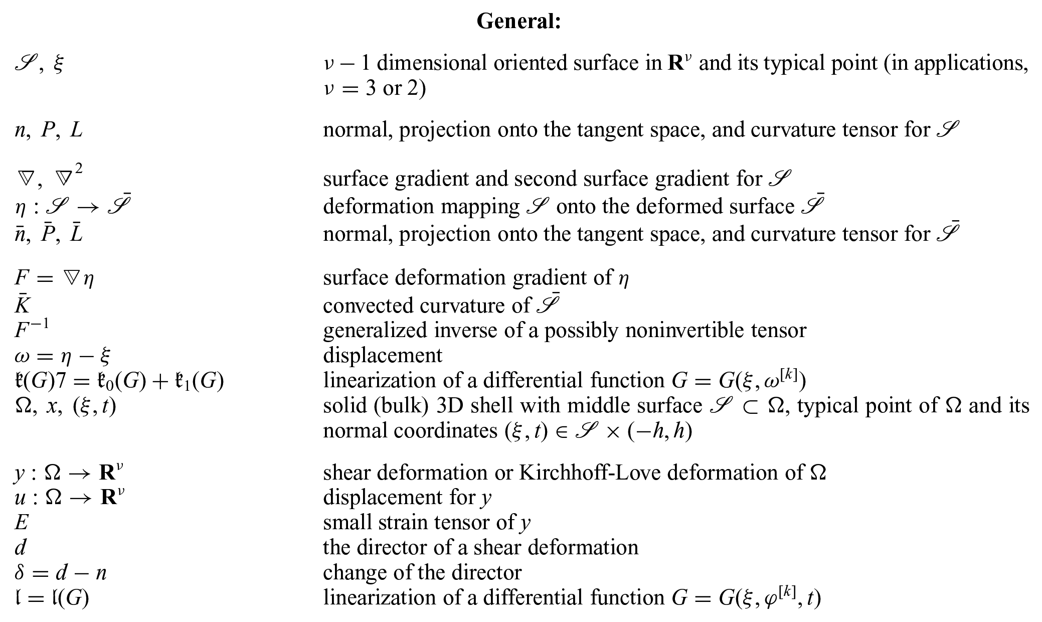
2. Glossary of notation

	General:
$S, ξ$	$ν - 1$ dimensional oriented surface in $R^{ν}$ and its typical point (in applications, $ν = 3$ or 2)
$n, P, L$	normal, projection onto the tangent space, and curvature tensor for $S$
$\nabla, \nabla^{2}$	surface gradient and second surface gradient for $S$
$η : S \to \bar{S}$	deformation mapping $S$ onto the deformed surface $\bar{S}$
$\bar{n}, \bar{P}, \bar{L}$	normal, projection onto the tangent space, and curvature tensor for $\bar{S}$
$F = \nabla η$	surface deformation gradient of $η$
$\bar{K}$	convected curvature of $\bar{S}$
$F^{- 1}$	generalized inverse of a possibly noninvertible tensor
$ω = η - ξ$	displacement
$k (G) 7 = k_{0} (G) + k_{1} (G)$	linearization of a differential function $G = G (ξ, ω^{[k]})$
$Ω, x, (ξ, t)$	solid (bulk) 3D shell with middle surface $S \subset Ω$ , typical point of $Ω$ and its normal coordinates $(ξ, t) \in S \times (- h, h)$
$y : Ω \to R^{ν}$	shear deformation or Kirchhoff-Love deformation of $Ω$
$u : Ω \to R^{ν}$	displacement for y
E	small strain tensor of y
d	the director of a shear deformation
$δ = d - n$	change of the director
$l = l (G)$	linearization of a differential function $G = G (ξ, φ^{[k]}, t)$

Review of the surface strain and bending strain tensors:

Shear deformations

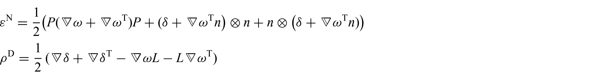
Present analysis: Naghdi’s surface strain $ε^{N}$ and a new bending strain tensor $ρ^{D}$ :

\begin{matrix} ε^{N} = \frac{1}{2} (P (\nabla ω + \nabla ω^{T}) P + (δ + \nabla ω^{T} n) \otimes n + n \otimes (δ + \nabla ω^{T} n)) \\ ρ^{D} = \frac{1}{2} (\nabla δ + \nabla δ^{T} - \nabla ω L - L \nabla ω^{T}) \end{matrix}

Naghdi: Naghdi’s surface strain $ε^{N}$ and Naghdi’s bending strain tensor $ρ^{N}$ :

ρ^{N} = \frac{1}{2} (\nabla δ + \nabla δ^{T} + L (\nabla ω + δ \otimes n) + (\nabla ω + δ \otimes n)^{T} L)

Kirchhoff-Love deformations

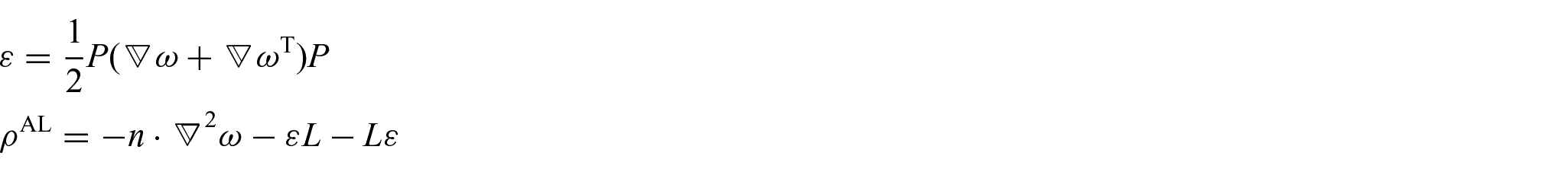
Present analysis: classical surface strain $ε$ and the Anicic-Léger bending strain tensor $ρ^{AL}$ :

\begin{matrix} ε = \frac{1}{2} P (\nabla ω + \nabla ω^{T}) P \\ ρ^{AL} = - n \cdot \nabla^{2} ω - ε L - L ε \end{matrix}

Koiter, Ciarlet: classical surface strain $ε$ and Koiter’s bending strain tensor $ρ^{K}$ :

ρ^{K} = - n \cdot \nabla^{2} ω

Budiansky-Sanders: classical surface strain $ε$ and Budiansky-Sanders bending strain tensor $ρ^{BS}$ :

ρ^{BS} = - n \cdot \nabla^{2} ω - \frac{1}{2} (ε L + L ε)

Invariant change of curvature

Present analysis: a new bending strain tensor $ρ^{C}$ :

ρ^{C} = - n \cdot \nabla^{2} ω - L (\nabla ω - \nabla ω^{T} n \otimes n) - (\nabla ω^{T} - n \otimes \nabla ω^{T} n) L

3. Geometry of surfaces, surface gradients of orders 1 and 2

This section presents the geometry of $ν - 1$ dimensional surfaces in $R^{ν}$ . Central to the approach are the first and second surface gradients as defined in [15], [14]. Our approach has many features in common with [11], [8], [6], [3], [4].

3.1. Surface and its tangent space

By a surface we mean an oriented $C^{2}$ manifold of dimension $ν - 1$ (without boundary) embedded in $R^{ν}$ . Thus a surface is a pair $(S, n)$ where $S \subset R^{ν}$ is the set of points and $n : S \to S^{ν - 1}$ is the unit normal giving the orientation, to be specified below. By definition, $S$ can be locally parametrized by a $C^{2}$ parametrization $π : dom π \to S$ . Specifically, we require that $π$ maps homeomorphically an open subset $dom π$ of $R^{ν - 1}$ onto a relatively open subset $ran π$ of $S$ and $\nabla π (λ)$ is an injective linear transformation from $R^{ν - 1}$ into $R^{ν}$ for every $λ \in dom π$ . The tangent space to $S$ at $ξ \in {cl}_{S}$ is the linear subspace of $R^{ν}$ of dimension $ν - 1$ given by

Tan (S, ξ) = ran \nabla π (λ) \equiv {\nabla π (λ) a : a \in R^{ν - 1}}

where $π$ is any local parametrization of $S$ such that $ξ = π (λ)$ for some $λ \in dom π$ . The normal in the pair $(S, n)$ is any continuous function $n : S \to S^{ν - 1}$ with values in the unit sphere such that $n (ξ)$ is perpendicular to $Tan (S, ξ)$ for every $ξ \in S .$ The class $C^{2}$ smoothness of $S$ implies that n is of class $C^{1} .$ We denote by $P (ξ)$ the orthogonal projection from $R^{ν}$ onto $Tan (S, ξ),$ given by

P = I - n \otimes n .

(13)

We often denote by $S$ the oriented surface $(S, n) .$

3.2. Definitions

Let $V$ be a finite dimensional vector space and $f : S \to V$ .

(i) We say that f is differentiable at $ξ \in S$ if f has an extension $\tilde{f} : U \to V$ to an n-dimensional neighborhood U of $ξ$ that is differentiable at $ξ .$ The surface gradient (= derivative) $\nabla f (ξ) \in Lin (R^{ν}, V)$ of f at $ξ$ is defined by

\nabla f (ξ) [a] = \nabla \tilde{f} (ξ) [P (ξ) a]

(14)

for any $a \in R^{ν}$ . This definition is independent of the choice of the extension. The element of $V$ defined by

\nabla_{a} f (ξ) : = \nabla f (ξ) [a]

is called the directional derivative of f at $ξ \in S$ in the direction $a \in R^{ν} .$

(ii) We say that f is twice differentiable at $ξ \in S$ if f is differentiable in some neighborhood of $ξ$ in $S,$ and $\nabla f$ has the derivative $\nabla (\nabla f) (ξ)$ at $ξ$ . We identify $\nabla (\nabla f) (ξ)$ with an equally denoted bilinear form given by

\nabla (\nabla f) (ξ) [a, b] = \nabla_{b} (\nabla_{a} f) (ξ) .

The form $\nabla (\nabla f) (ξ) [\cdot, \cdot]$ is not symmetric in general and should be distinguished from the second surface gradient of f. The second surface gradient of f at $ξ$ is a bilinear form $\nabla^{2} f (ξ)$ defined by

\nabla^{2} f (ξ) [a, b] = \nabla (\nabla f) (ξ) [Pa, b]

(15)

for any $a,$ $b \in R^{ν} .$ Proposition 3.4 shows that the form $\nabla^{2} f (ξ) [\cdot, \cdot]$ is symmetric; also it establishes the relation between $\nabla (\nabla f)$ and $\nabla^{2} f$ .

We interpret the second-order tensors as linear transformations from $R^{ν}$ into $R^{ν} .$ We denote the set of all second-order tensors by $Lin$ . Define the functions $L : S \to Lin$ and $κ : S \to R$ by

L = \nabla n, κ = {tr}_{L}

where $tr$ denotes the trace of a second-order tensor. We call L the curvature of $S$ and $κ$ the scalar curvature of $S$ . For the boundary $(S, n)$ of the unit ball oriented by the exterior normal n our choice of signs of L and $κ$ provides L a positive-semidefinite tensor and $κ$ a positive number. See Example 3.7.

3.3. Proposition

The curvature is symmetric and superficial, i.e.,

L = L^{T} and Ln = 0 .

(16)

Moreover, we have

\nabla_{b} Pa = - (n \cdot a) Lb - n (La \cdot b)

(17)

for any $a,$ $b \in R^{ν};$ equivalently,

\nabla P [b] = - Lb \otimes n - n \otimes Lb

for any $b \in R^{ν} .$

3.4. Proposition

If $f : S \to V$ is twice continuously differentiable then $\nabla^{2} f$ is symmetric, i.e.,

\nabla^{2} f [a, b] = \nabla^{2} f [b, a]

(18)

and we have

\nabla (\nabla f) [a, b] = \nabla^{2} f [a, b] - (n \cdot a) \nabla f [Lb] .

(19)

3.5. Lemma. (Normal extensions)

If $f : S \to V$ is a class $C^{2}$ function on $S$ then for each $x \in S$ there exists a class $C^{2}$ extension of f $\tilde{f} : U \to V$ defined on some neighborhood U of x in $R^{ν}$ such that

\nabla \tilde{f} (ξ) [n (ξ)] = 0 for every ξ \in S \cap U .

(20)

Proof. Let Z be the linear subspace of $R^{ν}$ given by

Z = {(x_{1}, \dots, x_{ν}) \in R^{ν} : x_{1} = x_{2} = \dots = x_{ν - 1} = 0} .

By [7, Subsection 3.1.19], each point of $S$ has a neighborhood U in $R^{ν}$ , a diffeomorphism $σ : U \to R^{ν}$ of class $C^{2}$ , and a relatively open subset $G$ of Z such that

σ (S \cap U) = G .

If $f : S \to V$ is a class $C^{2}$ function on $S$ then $g : = f ° σ^{- 1}$ is a class $C^{2}$ function on $G \subset Z .$ Let $\tilde{g} : G \times R \to V$ be given by

\tilde{g} (x_{1}, \dots, x_{ν}) = g (x_{1}, \dots, x_{ν - 1})

for any $(x_{1}, \dots, x_{ν}) \in G \times R .$ Then $\tilde{f} : = \tilde{g} ° σ$ has the required properties. □

Proof of Propositions 3.3 & 3.4. The properties (16) are well-known and their proof is omitted. To prove (17), we note that it is easy to verify that the directional surface gradient satisfies the product rule

\nabla_{a} (β \otimes γ) = (\nabla_{a} β) \otimes γ + β \otimes \nabla_{a} γ

for any $a \in R^{ν}$ and any two vector fields $β,$ $γ : S \to R^{ν} .$ Let $a,$ $b \in R^{ν}$ be fixed. From (13) we obtain

Pb = b - n (n \cdot b);

we then take the directional surface gradient $\nabla_{a}$ , use the product rule and the definition of L to obtain (17).

To prove (19), we take an arbitrary point x of $S$ , a class $C^{2}$ extension $\tilde{f}$ of f to a neighborhood of x in $R^{ν}$ satisfying (20) and a class $C^{1}$ extension $\tilde{P}$ of P to a neighborhood of x in $R^{ν}$ . We can assume that $\tilde{f}$ and $\tilde{P}$ are defined on the same neighborhood U of x. Throughout the proof let a and b be fixed vectors in $R^{ν} .$ The definition gives

\nabla f (ξ) [a] = \nabla \tilde{f} (ξ) [P (ξ) a]

(21)

for any $ξ \in S \cap U .$ Let $g_{a} : U \to V$ be defined by

g_{a} (η) = \nabla \tilde{f} (η) [\tilde{P} (η) a], η \in U .

(22)

A differentiation in the direction $\tilde{P} b$ yields

\nabla g_{a} [\tilde{P} b] = \nabla^{2} \tilde{f} [\tilde{P} a, \tilde{P} b] + \nabla \tilde{f} [\nabla (\tilde{P} a) [\tilde{P} b]]

(23)

throughout U. A comparison of the right-hand sides of (21) and (22) shows that $g_{a}$ is a class $C^{1}$ extension of $\nabla f [a]$ to U and hence the restriction of (23) to $S \cap U$ provides

\nabla (\nabla f [a]) [b] = \nabla^{2} \tilde{f} [Pa, Pb] + \nabla \tilde{f} [\nabla (Pa) [b]] .

(24)

The insertion of the formula

\nabla (Pa) [b] = - (n \cdot a) Lb - n (La \cdot b),

which is a consequence of (17), into the second term on the right-hand side of (24) and the use of (20) yields

\nabla (\nabla f [a]) [b] = \nabla^{2} \tilde{f} [Pa, Pb] - (n \cdot a) \nabla f [Lb] .

(25)

By (15) then

\nabla^{2} f [a, b] = \nabla^{2} \tilde{f} [Pa, Pb],

which proves (18) and reduces (25) to (19).

3.6. Example. (Surface gradients of the identity map)

Let $id : S \to R^{ν}$ be the identity map on $S$ given by

id (ξ) = ξ, ξ \in S .

(26)

Then

\nabla id = P, \nabla^{2} id = - n \otimes L .

(27)

Proof. The identity map ${id}_{R^{ν}}$ , given by ${id}_{R^{ν}} (η) = η$ for every $η \in R^{ν},$ is a local extension of $id$ . Then (14) provides $\nabla id = \nabla {id}_{R^{ν}} P = P,$ which is $(27)_{1}$ . From (17) we obtain

\nabla_{b} (\nabla_{a} id) = \nabla_{b} (Pa) = \nabla_{b} (a - n (n \cdot a)) = - Lb (n \cdot a) - n (La \cdot b),

which in combination with (15) yields $(27)_{2} .$ □

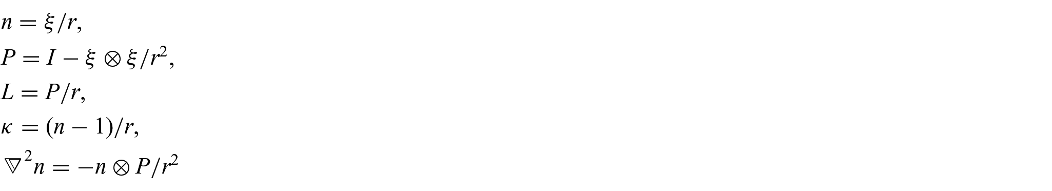
3.7. Example. (The curvature of a sphere)

Let $S = {ξ \in R^{ν} : | ξ | = r}$ be the sphere of radius $r > 0 .$ This is a surface of dimension $ν - 1$ of class $\infty$ and we have

\begin{matrix} n = ξ / r, \\ P = I - ξ \otimes ξ / r^{2}, \\ L = P / r, \\ κ = (n - 1) / r, \\ \nabla^{2} n = - n \otimes P / r^{2} \end{matrix}

where the quantities on the left-hand sides are evaluated at a general point $ξ \in S$ .

Proof. The expressions for n and P are immediate. To obtain the curvature, we use the local normal extension $\tilde{n}$ of n to $R^{ν}$ given by $\tilde{n} (η) = η / | η |$ for every $η \in R^{ν} \ {0} .$ Then $\nabla \tilde{n} (η) = (| η |^{2} - η \otimes η) / | η |^{3}$ and (14) yields $L = \nabla n = \nabla \tilde{n} = P / r .$ Next we note that for sphere $S$ we have $n = id / r$ and thus the expression for $\nabla^{2} n$ follows from $(27)_{2}$ . □

4. Deformation of a surface. Changes of the normal and curvature under deformation

This and the next sections determine the changes of the normal, projection onto the tangent space and curvature under the deformation of a surface. Here we treat exact formulas, the next section linearizations. The central results are the transformation formulas for the curvature in Proposition 4.4. As a preparation, we introduce the surface deformation gradient F and its generalized inverse $F^{- 1}$ as a particular case of the generalized of a non-invertible linear transformation to be introduced below.

4.1. Deformation of surfaces

Let $(S, n)$ be an oriented surface. We say that a map $η : S \to R^{ν}$ is a deformation of $S$ if $η$ is twice continuously differentiable, injective, and the surface deformation gradient of $η,$

F = \nabla η,

(28)

has the rank equal to $ν - 1$ everywhere on $S .$ It follows that the pair $(S, n)$ , given by

\bar{S} = η (S), \bar{n} ° η = | cof F |^{- 1} cof F n

(29)

is an oriented surface. Indeed, if $π : dom π \to S$ is a local parametrization of $S$ then $η ° π$ is a local parametrization of $\bar{S}$ ; moreover, the tangent space to $\bar{S}$ at $\bar{x} \in \bar{S}$ is given by

Tan (\bar{S}, \bar{x}) = F (ξ) Tan (S, ξ) where ξ = η^{- 1} (\bar{x}) .

To prove $(29)_{2}$ , we note that the tensor of cofactors is the unique continuous function $cof : Lin \to Lin$ satisfying $F^{T} cof F = (det F) I$ for every $F \in Lin$ . In the case (28), we have $F^{T} cof F = 0$ from which $cof F n \cdot Ft = 0$ for every $t \in Tan (S, ξ)$ and hence $cof F n \cdot \bar{t} = 0$ for every $\bar{t} \in Tan (\bar{S}, \bar{x}) .$

We call the pair $(\bar{S}, \bar{n})$ the image of $(S, n)$ under the deformation $η$ . The general unit normal to $\bar{S}$ is, of course, locally $\pm | cof F |^{- 1} cof F n$ , but our sign convention for the image is always as in $(29)_{2} .$

The formula

\bar{P} = I - \bar{n} \otimes \bar{n}

gives the projection onto the tangent space of $\bar{S} .$ We further denote by $\bar{L} : \bar{S} \to Lin$ the curvature of $\bar{S}$ , given by

\bar{L} = \nabla \bar{n},

where, of course, $\nabla$ denotes the surface differentiation with respect to $\bar{S} .$ Finally, we denote by $\bar{K} : S \to Sym$ the convected curvature, i.e., the pullback of $\bar{L}$ to $S,$ given by

\bar{K} = F^{T} (\bar{L} ° η) F .

4.2. Generalized inverse

To state the formulas that follow in a notationally simple form, we now introduce the generalized inverse of any $F \in Lin$ , invertible or not. Namely, we shall prove that for each $F \in Lin$ there exists a unique $F^{- 1} \in Lin$ such that

F^{- 1} F = P, F F^{- 1} = \bar{P} .

(30)

where P is the orthogonal projection onto the orthogonal complement $(\ker F)^{⊥}$ of the kernel of F and $\bar{P}$ is the orthogonal projection onto the range $ran F$ of $F .$ It suffices to note that F maps bijectively $(\ker F)^{⊥}$ onto $ran F$ and to put

F^{- 1} a = {\begin{matrix} F_{0}^{- 1} a & if & a \in ran F, \\ 0 & if & a \in {(ran F)}^{⊥}, \end{matrix}

where $F_{0}^{- 1} : ran F \to (\ker F)^{⊥}$ is the inverse of the restriction $F_{0}$ of F to $(\ker F)^{⊥} .$ Clearly,

F = FP = \bar{P} F, F^{- 1} = F^{- 1} \bar{P} = P F^{- 1},

(F^{- 1})^{- 1} = F .

If F is bijective, the generalized inverse coincides with the usual inverse of $F .$ One has $0^{- 1} = 0$ and $P^{- 1} = P$ for any orthogonal projection $P .$

If D is a $R^{ν}$ -valued bilinear form on $R^{ν} \times R^{ν}$ and $c \in R^{ν}$ a vector, we define the product $c \cdot D$ as a second-order tensor satisfying

(c \cdot D) a \cdot b = c \cdot D (a, b)

(31)

for every $a,$ and $b \in R^{ν} .$

4.3. Lemma

If $g : S \to R^{ν}$ is a $C^{2}$ function and $a \in R^{ν}$ a fixed vector then

\nabla (\nabla g^{T} a) = a \cdot \nabla^{2} g - n \otimes L \nabla g^{T} a

(32)

throughout $S .$

Proof. Let $f : S \to R$ be defined by $f (ξ) = g (ξ) \cdot a$ for every $ξ \in S .$ Then $\nabla f [b] = \nabla g [b] \cdot a = \nabla g^{T} a \cdot b$ for every $b \in R^{ν} .$ Hence (19) yields, for every $c \in R^{ν},$

\begin{matrix} \nabla_{c} (\nabla g^{T} a \cdot b) = \nabla_{c} (\nabla_{b} f) \\ = \nabla^{2} f [b, c] - (b \cdot n) \nabla f [Lc] \\ = a \cdot \nabla^{2} g [b, c] - (b \cdot n) (L \nabla g^{T} a \cdot c) \end{matrix}

(33)

where we have used $\nabla^{2} f = a \cdot \nabla^{2} g .$ Since b and c are arbitrary, we can restate (33) as (32). □

The following important proposition expresses the quantities $\bar{L}$ and $\bar{K}$ in terms of the second surface gradient of the deformation function $η$ .

4.4. Proposition

We have

\bar{L} ° η = - F^{- T} [(\bar{n} ° η) \cdot \nabla^{2} η] F^{- 1},

(34)

\bar{K} = - (\bar{n} ° η) \cdot \nabla^{2} η .

(35)

By (31), at each $ξ \in S,$ the right-hand sides of (34) and (35) are symmetric second-order tensors $S,$ T satisfying

a \cdot Sb = - \bar{n} (η) \cdot \nabla^{2} η [F^{- 1} a, F^{- 1} b],

a \cdot Tb = - \bar{n} (η) \cdot \nabla^{2} η [a, b],

for every $a,$ $b \in R^{ν},$ where the argument $ξ$ has been omitted.

Proof. Since the normal to the deformed surface is always in the orthogonal complement of F, we have the relation $F^{T} (\bar{n} ° η) = 0$ at every point $ξ$ of $S .$ The surface gradient of this relation provides

F^{T} \nabla (\bar{n} ° η) + (\nabla F^{T}) (\bar{n} ° η) = 0 .

We now apply (32) with $g = η$ to evaluate the second term to obtain

F^{T} (\nabla \bar{n} ° η) + (\bar{n} ° η) \cdot \nabla^{2} η - n \otimes L F^{T} (\bar{n} ° η) = 0 .

We multiply this equation by $F^{- 1}$ from the right and combine with the chain rule to obtain

F^{T} \bar{L} ° η + (\bar{n} ° η) \cdot (\nabla^{2} η) F^{- 1} - n \otimes F^{- T} L F^{T} (\bar{n} ° η) = 0 .

A multiplication from the right by $F^{- T}$ and the use of $F^{- T} n = 0$ gives (34). Equation (35) is a consequence. □

5. Linearized changes of the normal and curvature under deformation of a surface

This section gives approximate formulas for the changes of the normal, projection onto the tangent space and curvature under the deformation $η : S \to \bar{S}$ provided the displacement

ω (ξ) = η (ξ) - ξ, ξ \in S,

and its surface gradients up to some order k are small. We recall that by the results of Section 4 the quantities $\bar{n},$ $\bar{P},$ $\bar{L},$ and $\bar{K}$ can be expressed as functions of $η$ and its surface derivatives up to order $2 .$ Hence they can be expressed as functions of $ω$ and its surface derivatives up to order $2 .$

5.1. Differential functions of $(ξ, φ)$ ; linearization in the variable $φ^{[k]}$

Let $W$ and $V$ be finite dimensional vector spaces. If $φ : S \to W$ is a k-times continuously differentiable function and $ξ \in S,$ we denote by

φ^{[k]} (ξ) = (φ (ξ), \dots, \nabla^{k} φ (ξ))

(36)

the collection of surface derivatives of $φ$ at $ξ$ up to order k. Here $k = 0, 1, \dots$ Further, we denote by

J^{[k]} (S, W)

the set of all pairs $(ξ, φ^{[k]} (ξ))$ where $ξ$ ranges $S$ and $φ$ ranges the space $C^{k} (S, W)$ of all k-times continuously differentiable $W$ -valued functions on $S$ .

By a $V$ -valued differential function of $(ξ, φ)$ of order k we mean a continuously differentiable $V$ -valued function G on an open subset $dom G$ of $J^{[k]} (S, W)$ which contains all elements of the form $(ξ, 0^{[k]})$ where $ξ \in S$ . We write symbolically

G = G (ξ, φ^{[k]}) .

If $φ \in C^{k} (S, W)$ , then the equation

g (ξ) = G (ξ, φ^{[k]} (ξ)), ξ \in S,

determines the field g on $S$ corresponding to $φ .$

By the linearization of G in the variable $φ^{[k]}$ we mean a differential function $k (G)$ of $(ξ, φ)$ given by

k (G) (ξ, φ^{[k]}) = k_{0} (G) (ξ) + k_{1} (G) (ξ, φ^{[k]})

(37)

for every $(ξ, φ^{[k]}) \in J^{[k]} (S, W)$ where

k_{0} (G) (ξ) = G (ξ, 0), k_{1} (G) (ξ, φ^{[k]}) = \frac{dG (ξ, s φ^{[k]})}{ds} |_{s = 0} .

The assumption on $dom G$ guarantees that the arguments of G in the last two relations belong to $dom G$ (in the case of the second relation for all sufficiently small $| s |$ ). We write

G \approx k (G) as ω^{[k]} \to 0 .

Equation (37) shows that the function $k (G) (ξ, φ^{[k]})$ is affine in the variable $φ^{[k]}$ . The two terms on the right-hand side of (37) are the absolute and linear terms, respectively.

Let $V$ , $W$ and $X$ finite-dimensional vector spaces and let $(a, b) \to a ⊙ b$ be a bilinear operation from $V \times W$ into $X$ . The operation ⊙ can be, e.g., the product of two real numbers, scalar or tensor products, etc. Let G and H be differential functions with values in $V$ and $W$ . Then we have Leibniz’s rule

k_{1} (G ⊙ H) = k_{1} (G) ⊙ k_{0} (H) + k_{0} (G) ⊙ k_{1} (H) .

(38)

5.2. Lemma. (Linearized changes of the normal and tangential projection)

We have

\bar{n} \approx n - \nabla ω^{T} n,

(39)

\bar{P} \approx P + \nabla ω^{T} n \otimes n + n \otimes \nabla ω^{T} n

(40)

as $ω^{[1]} \to 0$ .

Equation (39) is standard; together with its consequence (40) it will be numerously used below.

Proof. Equation (39): We apply the operator $k_{1}$ to the equations

F^{T} \bar{n} = 0 and \bar{n} \cdot \bar{n} = 1 .

The use of Leibniz’s rule (38) and of the relations

k_{1} (F) = \nabla ω, k_{0} (F) = P, k_{0} (\bar{n}) = n,

then gives

\nabla ω^{T} n + P k_{1} (\bar{n}) \approx 0, n \cdot k_{1} (\bar{n}) \approx 0 .

The elimination of P from the first equation via $P = I - n \otimes n$ and the simplification of the result by the second equation provides

\nabla ω^{T} n + k_{1} (n) = 0

which is (39).

Equation (40) is obtained by the application of the operator $k_{1}$ to the equation $P = I - n \otimes n$ and the use of Leibniz’s rule in combination with (39). □

5.3. Theorem. (Linearized change of plain curvature)

We have

\bar{L} \approx L + ρ^{C} as ω^{[2]} \to 0

(41)

where $ρ^{C}$ is a second-order tensors given by

ρ^{C} = - n \cdot \nabla^{2} ω - L (\nabla ω - \nabla ω^{T} n \otimes n) - (\nabla ω^{T} - n \otimes \nabla ω^{T} n) L .

As mentioned in Introduction, Equation (41) and the tensor $ρ^{C}$ are new.

Proof. Recall the identity map $id : S \to R^{ν}$ from (26). The application of Leibniz’s rule (38) to the right-hand side of (34) gives

k_{1} (\bar{L}) = - k_{1} (F^{- T}) (n \cdot \nabla^{2} id) - k_{1} (\bar{n}) \cdot \nabla^{2} id - n \cdot \nabla^{2} ω - (n \cdot \nabla^{2} id) k_{1} (F^{- 1})

(42)

where we have used

k_{0} (\nabla^{2} η) = \nabla^{2} id, k_{1} (\nabla^{2} η) = \nabla^{2} ω

since $η = id + ω .$ We now linearize the individual terms occurring in (42). First, let us prove that

k_{1} (F^{- 1}) = - P \nabla ω + \nabla ω^{T} n \otimes n .

(43)

Indeed, the application of the operator $k_{1}$ to the equations $F^{- 1} F = P$ and $F^{- 1} \bar{n} = 0$ and Leibniz’s rule give

k_{1} (F^{- 1}) P + P \nabla ω = 0, k_{1} (F^{- 1}) n - \nabla ω^{T} n = 0 .

The elimination of P from the first equation via $P = I - n \otimes n$ and the simplification of the result by the second equation provides (43). Further, Equations $(27)_{2}$ and (39) provide

n \cdot \nabla^{2} id = - L, k_{1} (\bar{n}) \cdot \nabla^{2} id = 0 .

(44)

The insertion of (43) and (44) into (42) gives (41).

5.4. Theorem. (Linearized change of the convected curvature)

We have

\bar{K} \approx L + ρ^{K} as ω^{[2]} \to 0

(45)

where $ρ^{K}$ is a second-order tensor given by

ρ^{K} = - n \cdot \nabla^{2} ω .

(46)

The tensor $ρ^{K}$ is called the Koiter bending strain tensor. The compact expression in (46) is equivalent to the original component expression by Koiter [10, Eq. (3.4)]. The equivalence can be established by a straightforward computation; however, a more direct way is employed here. Namely, Koiter defines the covariant components of $ρ^{K}$ as the linearization of the difference of components of $\bar{L}$ and L in the convected and original coordinate systems, respectively. That property of $ρ^{K}$ is proved in Theorem 5.8 (below).

Proof. Equation (45): We linearize (35) by Leibniz’s rule to obtain

k_{1} (\bar{K}) = - k_{1} (\bar{n}) \cdot \nabla^{2} id = - n \cdot \nabla^{2} ω .

(47)

Equations $(27)_{2}$ and (39) provide $k_{1} (\bar{n}) \cdot \nabla^{2} id = 0$ and thus (47) reduces to (45). □

5.5. Coordinates and convected coordinates

Let $π : dom π \to S$ be a local parametrization of $S$ defined on an open subset $dom π$ of $R^{ν - 1}$ (Section 3.1). Each $ξ \in S$ that belong also to the range $ran π$ of $π$ can be written as $ξ = π (x^{1}, \dots, x^{ν - 1})$ where $(x^{1}, \dots, x^{ν - 1}) \in dom π$ are called local coordinates of $ξ .$ Let $a_{α} : ran π \to R^{ν}$ be the coordinate vectors, i.e.,

a_{α} ° π = \partial π / \partial x^{i}, a_{α} (ξ) \in Tan (S, ξ), α = 1, \dots, ν - 1,

and let $a^{α}$ be the dual basis (in the tangent space). If $η : S \to \bar{S}$ is a deformation, then each point $\bar{ξ} \in \bar{S} \cap η (ran π)$ can be written as $\bar{ξ} = η (π (x^{1}, \dots, x^{ν - 1}))$ where $(x^{1}, \dots, x^{ν - 1}) \in dom π$ are called convected local coordinates of $\bar{ξ} .$ We denote by ${\bar{a}}_{α} (\bar{ξ}),$ ${\bar{a}}^{α} (\bar{ξ}) \in Tan (\bar{S}, \bar{ξ})$ the coordinate vectors corresponding to the convected coordinates. Clearly,

{\bar{a}}_{α} ° η = F a_{α}, {\bar{a}}^{α} ° η = F^{- T} a^{α}

where F is the deformation gradient of $η .$ Let $L_{α β}$ be the components of L in the basis $a^{α}$ and let ${\bar{L}}_{α β}$ be the components of $\bar{L}$ in the basis ${\bar{a}}^{α}$ of the convected coordinate system i.e.,

L = L_{α β} a^{α} \otimes a^{β}, \bar{L} = {\bar{L}}_{α β} {\bar{a}}^{α} \otimes {\bar{a}}^{β},

where we use the summation convention.

5.6. Components of linearization versus linearization of components

It is important to realize that the components of the linearization of the curvature tensor differ from the linearization of the components of the curvature tensor. The reason is that the former takes into account changes of coordinate vectors while the latter not.

We now determine the difference explicitly for a general quantity. Let $\bar{S}$ be a $Lin$ -valued differential function of $(ξ, ω)$ of order $k \geq 1$ such that $\bar{S} (ξ, ω^{[k]})$ is a symmetric linear transformation from $Tan (S, ξ)$ into itself. To introduce the components of $\bar{S}$ as differential functions of $(ξ, ω),$ we first define ${\bar{a}}^{α}$ as a differential function of $(ξ, ω)$ of order 1 by

{\bar{a}}^{α} (ξ, ω^{[1]}) = F^{- T} a^{α}

(48)

for any $(ξ, ω^{[1]}) \in J^{[k]} (S, R^{n})$ where $F = P (ξ) + \nabla ω (ξ)$ and $a^{α} = a^{α} (ξ) .$ Then we define differential functions ${\bar{S}}_{α β}$ of $(ξ, ω)$ of order k by

\bar{S} (ξ, ω^{[k]}) = {\bar{S}}_{α β} (ξ, ω^{[k]}) {\bar{a}}^{α} \otimes {\bar{a}}^{β}

for any $(ξ, ω^{[k]}) \in J^{[k]} (S, R^{n})$ , where ${\bar{a}}^{α}$ and ${\bar{a}}^{β}$ are evaluated at $(ξ, ω^{[1]}) .$

5.7. Proposition

For any $(ξ, ω^{[k]}) \in J^{[k]} (S, R^{n})$ we have

\begin{matrix} k ({\bar{S}}_{α β} {\bar{a}}^{α} \otimes {\bar{a}}^{β}) - k ({\bar{S}}_{α β}) a^{α} \otimes a^{β} \\ = (n \otimes \nabla ω^{T} n - \nabla ω^{T}) S + S (\nabla ω^{T} n \otimes n - \nabla ω); \end{matrix}

(49)

where $S = \bar{S} (ξ, 0^{[k]})$ and $\nabla ω$ and n are evaluated at $ξ$ .

Proof. Since the absolute terms of the two linearizations on the left-hand side of (49) coincide, it suffices to compute the difference of the linear terms. If we view the term ${\bar{S}}_{α β} {\bar{a}}^{α} \otimes {\bar{a}}^{β}$ as the product of ${\bar{S}}_{α β}$ with ${\bar{a}}^{α} \otimes {\bar{a}}^{β}$ , Leibniz’s rule (38) gives

k_{1} ({\bar{S}}_{α β} {\bar{a}}^{α} \otimes {\bar{a}}^{β}) = k_{1} ({\bar{S}}_{α β}) a^{α} \otimes a^{β} + S_{α β} k_{1} ({\bar{a}}^{α} \otimes {\bar{a}}^{β}) .

(50)

By (48) we obtain $k_{1} ({\bar{a}}^{α}) = k_{1} (F^{- T}) a^{α} .$ Using (43) to compute $k_{1} (F^{- T})$ , we obtain

k_{1} ({\bar{a}}^{α}) = n (n \cdot \nabla ω^{T} n) - \nabla ω^{T} {\bar{a}}^{α} .

(51)

By Leibniz’s rule

k_{1} ({\bar{a}}^{α} \otimes {\bar{a}}^{β}) = k_{1} ({\bar{a}}^{α}) \otimes a^{β} + a^{α} \otimes k_{1} ({\bar{a}}^{β}) .

(52)

The insertion of (51) into (52) and the insertion of the result into (50) then gives (49). □

5.8. Theorem. (Linearized changes of components of the curvature tensor)

We have

{\bar{L}}_{α β} \approx L_{α β} + ρ_{α β}^{K} as ω^{[2]} \to 0,

(53)

where $ρ_{α β}^{K}$ are the components of $ρ^{K}$ in the basis $a^{α}$ .

As already mentioned, Property (53) is used as the definition of $ρ^{K}$ in [10, Eq. (3.4)]. It is also employed in [5, Section 2.5].

Proof. The particular case $S = L$ in (49) gives

k (\bar{L}) - k ({\bar{L}}_{α β}) a^{α} \otimes a^{β} = (n \otimes \nabla ω^{T} n - \nabla ω^{T}) L + L (\nabla ω^{T} n \otimes n - \nabla ω) .

(54)

By (41) we have $k (\bar{L}) = L + ρ^{C}$ and the elimination of $k (\bar{L})$ from (54) provides

k ({\bar{L}}_{α β}) a^{α} \otimes a^{β} = L_{α β} a^{α} \otimes a^{β} - n \cdot \nabla^{2} ω

which completes the proof of (53). □

The eigenvalues of the curvature tensor L are called the principal curvatures of $S$ . We recall that L is superficial, i.e., $Ln = 0$ and hence at least one eigenvalue of L is equal to $0 .$ The remaining eigenvalues are denoted by $κ_{1} \geq \dots \geq κ_{ν - 1},$ where in this descending sequence we take into account multiplicities. We define the principal curvatures ${\bar{κ}}_{1} \geq \dots \geq {\bar{κ}}_{ν - 1}$ of $\bar{S}$ analogously.

5.9. Theorem. (Linearized changes of principal curvatures, Anicic [1])

Let $S$ have distinct principal curvature $κ_{α},$ $α = 1, \dots, ν - 1,$ with the corresponding normalized eigenvectors of L denoted by $e_{α}$ . Then the linearizations of the principal curvatures of $\bar{S}$ are

{\bar{κ}}_{α} \approx κ_{α} + ρ^{C} e_{α} \cdot e_{α} \equiv κ_{α} + ρ^{AL} e_{α} \cdot e_{α}

(55)

as $ω^{[2]} \to 0$ , where $ρ^{AL}$ is a second-order tensor given by

ρ^{AL} = - n \cdot \nabla^{2} ω - ε L - L ε .

(56)

Proof. Since the principal curvatures ${\bar{κ}}_{α}$ are the eigenvalues of $\bar{L},$ which we write as ${\bar{κ}}_{α} = {\hat{κ}}_{α} (\bar{L})$ , the well-known continuity and differentiability properties of eigenvalues of a symmetric tensor (see, e.g., [9, Eq. (6.10), p. 125] or [16, Section 2, Eq. (2.1)]) show that ${\hat{κ}}_{α} (\bar{L})$ are Lipschitz continuous functions of $\bar{L}$ and if ${\hat{κ}}_{α} (L)$ is a simple eigenvalue of $L,$ then ${\hat{κ}}_{α} (\bar{L})$ is infinitely differentiable in some neighborhood of L and the derivative at L is given by

D_{{\hat{κ}}_{α}} (L) [B] = B e_{α} \cdot e_{α}

for every symmetric $B \in Lin$ where $e_{α}$ is the corresponding unit eigenvector of L. The last formula in combination with the chain rule and (41) gives

k_{1} ({\bar{κ}}_{α}) = k_{1} (\bar{L}) e_{α} \cdot e_{α} = ρ^{AL} e_{α} \cdot e_{α} .

Observing that $ρ^{C} e_{α} \cdot e_{α} = ρ^{AL} e_{α} \cdot e_{α},$ we obtain (55).

5.10. Example. (Comparison of linearized curvature tensors)

We consider an isotropic expansion the sphere $S$ of radius $r > 0$ and center 0 in $R^{ν}$ into the sphere $\bar{S}$ of radius $\bar{r} > r$ and of the same center. This changes the curvature tensor L and scalar curvature $κ$ of $S$ into the corresponding quantities $\bar{L}$ and $\bar{κ}$ of $\bar{S}$ . We calculate the differences

\bar{L} - L, \bar{κ} - κ

(57)

directly from the definitions and then, assuming that the difference $Δ r : = \bar{r} - r$ is small, we linearize the quantities (57) in $Δ r .$ The goal is to compare these linearized changes with the ‘predictions’ given by $ρ^{K},$ $ρ^{BS},$ $ρ^{AL},$ and $ρ^{C}$ .

By Example 3.7,

L = P / r, κ = (n - 1) / r, \bar{L} = \bar{P} / \bar{r}, \bar{κ} = (n - 1) / \bar{r};

here P and $\bar{P}$ are the projections onto the tangents spaces of $S$ and $\bar{S};$ the tensors L and P are evaluated at a general point $ξ \in S$ and the tensors $\bar{L}$ and $\bar{P}$ at the point $\bar{ξ} = (\bar{r} / r) ξ \in \bar{S} .$ Consequently,

\bar{L} (\bar{ξ}) - L (ξ) = (1 / \bar{r} - 1 / r) P (ξ), \bar{κ} - κ = (n - 1) (1 / \bar{r} - 1 / r) .

The linearizations in $Δ r : = \bar{r} - r$ are

1 / \bar{r} - 1 / r \approx - Δ r / r^{2},

\bar{L} (\bar{ξ}) - L (ξ) \approx - (Δ r / r^{2}) P (ξ), \bar{κ} - κ \approx - (n - 1) Δ r / r^{2} .

(58)

We now interpret the correspondence $ξ \to \bar{ξ} = (\bar{r} / r) ξ$ as a deformation $η$ of the sphere $S$ into the sphere $\bar{S} .$ Thus the deformation and the displacement are

η (ξ) = (\bar{r} / r) ξ and ω (ξ) = Δ r n (ξ) for every ξ \in S .

From the equation $\nabla^{2} n = - n \otimes P / r^{2}$ (see Example 3.7) we obtain

\nabla^{2} ω = - (Δ r / r) n \otimes L = - (Δ r / r^{2}) n \otimes P

and from that we deduce

ρ^{K} = (Δ r / r^{2}) P, ρ^{BS} = 0, ρ^{C} = ρ^{AL} = - (Δ r / r^{2}) P .

(59)

In view of (58), only $ρ^{AL}$ and $ρ^{C}$ give the correct result. In particular, (59)₁ gives

tr ρ^{K} = (ν - 1) Δ r / r^{2},

which is positive if $Δ r$ is positive. Thus $ρ^{K}$ predicts an increase of the mean curvature under a genuine increase of the radius $r \to \bar{r} = r + Δ r > r .$

5.11. Lemma

For any oriented surface $(S, n)$ we have

n \cdot \nabla^{2} n = - L^{2} .

(60)

Proof. Since $\nabla n = L$ is symmetric and superficial, we have $n \cdot \nabla n [a] \equiv n \cdot La = 0$ for any $a \in R^{ν}$ . A differentiation of the relation $n \cdot \nabla n [a] = 0$ in the direction $b \in R^{ν}$ provides

\nabla n [b] \cdot \nabla n [a] + n \cdot \nabla (\nabla n) [a, b] = 0 .

(61)

By (19) we have

\nabla (\nabla n) [a, b] = \nabla^{2} n [a, b] - (n \cdot a) L^{2} b

and consequently,

n \cdot \nabla (\nabla n) [a, b] = n \cdot \nabla^{2} n [a, b] .

The insertion of this into (61) and the omission of the arguments $a,$ $b,$ yields (60). □

5.12. Example. (Normal expansion of a surface)

The preceding example can be generalized. Let $(S, n)$ be an oriented surface, let $s > 0$ be a given number, and consider a subset $\bar{S}$ of $R^{ν}$ and a map $η : S \to R^{ν}$ given by

\begin{matrix} \bar{S} = {ξ + sn (ξ) : ξ \in S}, \\ η (ξ) = ξ + sn (ξ), ξ \in S . \end{matrix}

If $s > 0$ is sufficiently small, the implicit function theorem can be used to prove that the map $η$ is injective. Moreover, if $\bar{n} : \bar{S} \to R^{ν}$ is defined by

\bar{n} (\bar{ξ}) = n (η^{- 1} (\bar{ξ})), \bar{ξ} \in \bar{S},

(62)

then $\bar{n}$ is normal to $\bar{S}$ and thus $(\bar{S}, \bar{n})$ is an oriented surface. We now determine the curvature of $\bar{S} .$ One possibility is to use the general formula (34) ; however, in view of (62), it is simpler to use directly the definition of curvature. Namely, we have

\bar{L} ° η = \nabla \bar{n} ° η = \nabla (\bar{n} ° η) F^{- 1} = \nabla n F^{- 1}

where $F = P + sL$ is the surface deformation gradient of $η$ and

F^{- 1} = (P + sL)^{- 1}

its generalized inverse. Thus

\bar{L} ° η = L (P + sL)^{- 1} .

Thus the change of curvature under the passage from $S$ to $\bar{S}$ is

\bar{L} - L = L (P + sL)^{- 1} - L

where $\bar{L}$ is evaluated at $η (ξ)$ and the remaining quantities at $ξ .$ It is easy to verify that $\bar{L} - L$ is negative semidefinite if $t > 0 .$ Thus a normal expansion of $S$ can only decrease the curvature, an intuitively clear fact. The linearized change of curvature is

\bar{L} - L \approx - s L^{2} .

The displacement of the deformation $η$ is

ω = sn .

The elimination of the term $n \cdot \nabla^{2} ω \equiv sn \cdot \nabla^{2} n$ by (60) from the formulas for $ρ^{K},$ $ρ^{BS},$ $ρ^{AL},$ and $ρ^{C}$ provides

ρ^{K} = s L^{2}, ρ^{BS} = 0, ρ^{C} = ρ^{AL} = - s L^{2} .

Thus the conclusion is the same as that in Example 5.10: only $ρ^{AL}$ and $ρ^{C}$ give the correct result.

6. Shell-like bodies

The following notion is central for this and the next sections.

A shell-like body is a subset $Ω$ of $R^{ν}$ of the form

Ω : = {x = ξ + tn (ξ) : ξ \in S, - h < t < h},

where $(S, n)$ is an $ν - 1$ -dimensional oriented surface and h a positive number. For technical reasons we assume that $S$ is bounded and that there exists a $C^{2}$ oriented surface $\tilde{S}$ such that the closure ${cl}_{S}$ of $S$ in $R^{ν}$ satisfies ${cl}_{S} \subset \tilde{S}$ . We call $S$ the middle surface of $Ω$ and $2 h$ the thickness of $Ω$ . As before, we denote by $P,$ $L : S \to Lin$ the projection onto the tangent space of $S$ , and the curvature of $S,$ respectively.

6.1. Proposition. (Normal coordinates)

If the thickness of a shell-like body $Ω$ is sufficiently small then the map $x_{°} : S \times (- h, h) \to R^{ν}$ defined by

x_{°} (ξ, t) = ξ + tn (ξ), (ξ, t) \in S \times (- h, h),

(63)

is a diffeomorphism onto $Ω$ . The inverse map associates with any $x \in Ω$ an element of $S \times (- h, h)$ which we denote by $(ξ_{°} (x), t_{°} (x))$ . We have

\nabla ξ_{°} (x) = (P (ξ) + tL (ξ {))}^{- 1}, \nabla t_{°} (x) = n (ξ)

(64)

for any $x \in Ω,$ where $ξ = ξ_{°} (x)$ and where the right-hand side of $(63)_{1}$ is the generalized inverse of the noninvertible tensor $P + tL,$ see Subsection 4.2. We call the parameters $ξ_{°} (x), t_{°} (x)$ the normal coordinates of $x .$

Throughout this chapter, $Ω$ denotes a shell-like body that admits normal coordinates $(ξ_{°}, t_{°}) .$

Proof. The normal coordinates are solutions of the equation

x = ξ_{°} (x) + t_{°} (x) n (ξ_{°} (x))

(65)

Let $\tilde{S}$ be the extension of ${cl}_{S}$ as in the definition of a shell-like body. Consider an extension ${\tilde{x}}_{°} : \tilde{S} \times (- h, h) \to R^{ν}$ of $x_{°}$ given by the right-hand side of (63) for every $(ξ, t) \in \tilde{S} \times (- h, h) .$ The derivative of ${\tilde{x}}_{°}$ at $ξ \in \tilde{S}$ and $t = 0$ is given by

\nabla {\tilde{x}}_{°} (ξ, 0) (a, b) = P (ξ) a + b \bar{n} (ξ)

for every $a \in Tan (\tilde{S}, ξ)$ and $b \in R,$ where we have used that the surface gradient of the identity map ${id}_{\tilde{S}}$ on $\tilde{S}$ is $\nabla {id}_{\tilde{S}} = P,$ see (27). From the definition of a surface one readily deduces that $\nabla {\tilde{x}}_{°} (ξ, 0)$ maps $R^{ν}$ bijectively onto $R^{ν}$ for any $ξ \in \tilde{S} .$ Thus by the inverse function theorem, for every point $ξ \in \tilde{S}$ , ${\tilde{x}}_{°}$ has a continuously differentiable inverse ${\tilde{x}}_{°}^{- 1} : O_{ξ} \to \tilde{S} \times R$ defined in some neighborhood of $ξ$ . Since ${cl}_{S}$ is compact, a standard compactness argument shows that ${\tilde{x}}_{°}$ is invertible in some neighborhood of ${cl}_{S} .$ Hence $x_{°}$ has a continuously differentiable inverse in $Ω$ if h is sufficiently small. To prove (64), we differentiate (65) in the direction $c \in R^{ν} .$ The definition of L provides

c = \nabla ξ_{°} [c] + \nabla t_{°} [c] n (ξ_{°}) + t_{°} L (ξ_{°}) \nabla ξ_{°} [c]

where we have omitted the argument $x .$ Splitting the last equation into the tangential and normal components and solving for $\nabla ξ_{°} (x)$ and $\nabla t_{°} (x)$ we obtain (64). □

7. Linearized strain tensors: the shear and Kirchhoff-Love’s cases

This section deals with shear deformations and Kirchhoff-Love’s deformations of a shell-like body of $Ω$ . The strain tensor E is determined for these two types of deformations as functions of the normal coordinates $(ξ, t)$ of a point $x \in Ω .$ The objective is to linearize E under the assumption that t and the displacement are small.

7.1. Shear deformations

A map $y : Ω \to R^{ν}$ is said to be a shear deformation if

y (x) = η (ξ) + td (ξ)

for any $x \in Ω$ with the normal coordinates $(ξ, t)$ , where $η : S \to R^{ν}$ is a deformation of $S$ (see Subsection 4.1) and $d : S \to R^{ν}$ is a map.

The function d gives the direction after the deformation of the material line that was normal to the middle surface before the deformation.

The bulk displacement u and the bulk strain tensor E of any deformation are given by

u (x) = y (x) - x, x \in Ω,

(66)

and

E = \frac{1}{2} (\nabla u + \nabla u^{T}) .

One obtains

u (x) = ω (ξ) + t δ (ξ)

where $(ξ, t)$ are the normal coordinates of $x \in Ω$ and

ω (ξ) = η (ξ) - ξ, δ (ξ) = d (ξ) - n (ξ)

(67)

are the displacement of the middle surface and the change of $d,$ respectively. A differentiation of u given by (66) using equations (64) provides

\nabla u = (\nabla ω + t \nabla δ) (P + tL)^{- 1} + δ \otimes n .

(68)

The derivative $\nabla u$ in (68), and hence also its symmetrization $E,$ depends explicitly on $\nabla ω,$ $\nabla δ$ and t, and implicitly on $ξ$ through the quantities n, P and $L .$ Using the notation (36), we can say that $\nabla u$ and E depend on $(ξ, ω^{[1]}, δ^{[1]}, t) .$ Similarly, it will be seen in (84) (below) that in the Kirchhoff-Love case $\nabla u$ depends on $(ξ, ω^{[2]}, t)$ . Below, these dependencies are unified in the notion of a differential function of $(ξ, φ, t)$ of order $k,$ where $φ$ is a function with values in a finite dimensional vector space. A differential function G of $(ξ, φ, t)$ of order k is an ordinary function of the variables $(ξ, φ^{[k]}, t)$ . The function G is generally nonlinear in the variables $(φ^{[k]}, t) .$ If $φ^{[k]}$ and t are small, we can replace the exact dependence of G on $(φ^{[k]}, t)$ by the linearization of G in the variables $(φ^{[k]}, t)$ (‘small displacements of thin shells’).

7.2. Differential functions of $(ξ, φ, t)$ ; linearization in the variables $(φ^{[k]}, t) .$

Let $W$ and $V$ be finite dimensional vector spaces. We denote by

J^{[k]} (S, W, R)

the set of all triples $(ξ, φ^{[k]} (ξ), t)$ , where $ξ$ ranges $S$ , $φ$ ranges $C^{k} (S, W)$ , and t ranges $R .$ We refer to (36) for the definition of $φ^{[k]} (ξ) .$ Here $k = 0, 1, \dots$

By a $V$ -valued differential function of $(ξ, φ, t)$ of order k we mean a continuously differentiable $V$ -valued function G on an open subset $dom G$ of $J^{[k]} (S, W, t)$ which contains all elements of the form $(ξ, 0^{[k]}, 0)$ , where $ξ \in S$ . We write symbolically

G = G (ξ, φ^{[k]}, t) .

If $Ω$ is a shell-like body, then any $φ \in C^{k} (S, W)$ determines a field g on $Ω$ by putting

g (x) = G (ξ, φ^{[k]} (ξ), t)

for a general point $x \in Ω$ with normal coordinates $(ξ, t)$ .

The linearization of G in the variables $(φ^{[k]}, t)$ is a differential function $l (G)$ of $(ξ, φ, t)$ of order $k .$ The procedure consists of two steps. The first step is the linearization $k$ of $G (ξ, φ^{[k]}, t)$ in the variable $φ^{[k]}$ , defined in Subsection 5.1. The second step is the linearization in the variable t. If H is a function of t defined on an open subset of $R$ which contains the origin, we define its linearization in the variable t as the function $t (H)$ on $R$ by

t (H) (t) = H (0) + \frac{dH (τ t)}{d τ} |_{τ = 0} .

(69)

A formal definition of the linearization of $G = G (ξ, φ^{[k]}, t)$ in the variables $(φ^{[k]}, t)$ is as follows. Given $t \in R,$ we define a differential function $G_{t}$ of $(ξ, φ)$ by

G_{t} (ξ, φ^{[k]}) = G (ξ, φ^{[k]}, t)

and determine the linearization $k (G_{t})$ of $G_{t}$ in the variable $φ^{[k]},$ which is again a differential function of $(ξ, φ)$ , as defined in Subsection 5.1. To proceed to the linearization in the variable $t,$ for each $ξ, φ$ we define the function $H_{ξ, φ}$ of t by

H_{ξ, φ} (t) = k (G_{t}) (ξ, φ^{[k]}) .

The linearization of G in $(φ, t)$ is a differential function $l (G)$ of $(ξ, φ^{[k]}, t)$ given by

l (G) (ξ, φ^{[k]}, t) = t (H_{ξ, φ})

for every $(ξ, φ^{[k]}, t) \in J^{[k]} (S, W, R) .$ We write

G \approx l (G) as (φ^{[k]}, t) \to 0 .

The definition implies that for every $ξ \in S$ , the function $l (G) (ξ, φ^{[k]}, t)$ is affine in t at fixed $φ^{[k]}$ and affine in $φ^{[k]}$ at fixed $t .$ Hence $l (G)$ is the sum

l (G) (ξ, φ^{[k]}, t) = A (ξ) + B (ξ, φ^{[k]}) + C (ξ, t) + D (ξ, φ^{[k]}, t)

(70)

where the four terms on the right-hand side of (70) are the absolute term, the term linear in $φ^{[k]},$ the term linear in $t,$ and the term bilinear in the pair of variables $(φ^{[k]}, t) .$ These functions are given in (93) (below) in terms of G and its partial derivatives.

We now apply this formalism to $φ = (ω, δ)$ and to a differential function given by the right-hand side of (68).

7.3. Proposition

We have the following approximate formula for the strain tensor E of a shear deformation at a point $x \in Ω$ with normal coordinates $(ξ, t)$ :

E \approx ε^{N} + t ρ^{D} as (ω^{[1]}, δ^{[1]}, t) \to 0,

(71)

where

ε^{N} = \frac{1}{2} (\nabla ω + \nabla ω^{T} + δ \otimes n + n \otimes δ),

(72)

ρ^{D} = \frac{1}{2} (\nabla δ + \nabla δ^{T} - \nabla ω L - L \nabla ω^{T})

(73)

where all quantities are evaluated at $ξ .$

Proof. Let G be a differential function of order 1 of $φ : = (ω, δ)$ given by

G (ξ, φ^{[1]}, t) = (\nabla ω + t \nabla δ) (P + tL)^{- 1} + δ \otimes n .

(74)

Since the right-hand side of (74) is linear in $φ^{[1]}$ , it coincides with its linearization. Next, to linearize the right-hand side of (74) in the variable $t,$ we note that the absolute and linear terms of the linearization are

\nabla ω + δ \otimes n

and

\frac{d [(\nabla ω + τ t \nabla δ) (P + τ tL)^{- 1}]}{d τ} |_{τ = 0},

(75)

respectively. To use the product rule to calculate the derivative in (75), let us preliminarily prove that

\frac{d {(P + tL)}^{- 1}}{dt} |_{t = 0} = - L .

(76)

Indeed, if $t \in R$ is sufficiently close to 0 then $\ker (P + tL) = n^{⊥}$ is the orthogonal complement of n and hence $(\ker (P + tL {))}^{⊥} = ran P .$ Thus, invoking the definition of the generalized inverse, we see that $(30)_{1}$ reads

(P + tL)^{- 1} (P + tL) = P .

The differentiation at $t = 0$ gives (76). The calculation of the derivative in (75) provides $t (\nabla δ - \nabla ω) L .$ Hence the linearization of the right-hand side of (74) in the variable t is

\nabla ω + δ \otimes n + t (\nabla δ - \nabla ω) L

which also $l (G) (ξ, φ^{[k]} (ξ), t)$ by definition. Thus

\nabla u \approx \nabla ω + δ \otimes n + t (\nabla δ - \nabla ω L) as (ω^{[1]}, δ^{[1]}, t) \to 0 .

A symmetrization gives (71), (72) and (73). □

7.4. Remark

In [12, Equation (7.69)] Naghdi derives a different approximate expression for the components $γ_{ij}^{*}$ of $E .$ In our notation, he derives

E \approx ε^{N} + t ρ^{N} as (ω^{[1]}, δ^{[1]}, t) \to 0,

(77)

where $ε^{N}$ is as before, but

ρ^{N} = \frac{1}{2} (\nabla δ + \nabla δ^{T} + L (\nabla ω + δ \otimes n) + (\nabla ω + δ \otimes n)^{T} L),

(78)

which is called Naghdi’s bending strain tensor in the literature. It is often used with the additional realistic restriction $δ \cdot n = 0,$ in which case we have [5, p. 365], [4]

ρ^{N} = \frac{1}{2} (P \nabla δ + \nabla δ^{T} P + L \nabla ω + \nabla ω^{T} L) .

(79)

The difference between the tensors in (78) and (73) is found to be

ρ^{N} - ρ^{D} = ε^{N} L + L ε^{N}

The following example is devoted to this discrepancy.

7.5. Example

Let $Ω$ be a solid spherical shell with the middle surface $S^{ν - 1}$ and the thickness $2 h$ , $0 < h < 1$ , i.e.,

Ω = {x \in R^{ν} : | | x | - 1 | < h} .

Let $y : Ω \to R^{ν}$ be a deformation and the corresponding displacement $u : Ω \to R^{ν}$ given by

y (x) = cx / | x | + x and u (x) = cx / | x |, x \in Ω,

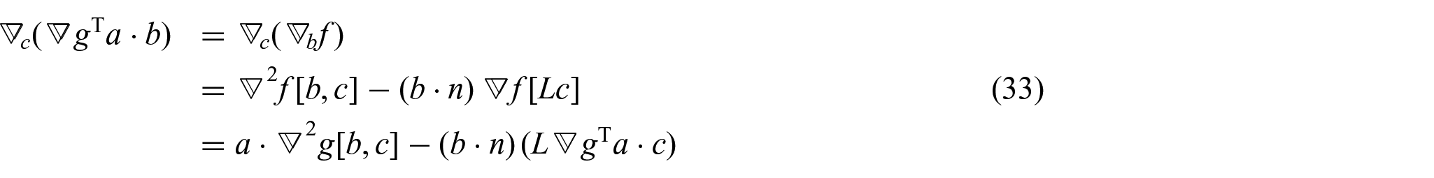
where c is a constant. Our goal is to compute the strain tensor of u, then to linearize in c under the assumption that c is small, and finally to compare the result with the ‘predictions’ for this linearization given by $ρ^{D}$ and $ρ^{N} .$

The strain tensor of the displacement $ω$ is

E (x) = \nabla u (x) = \frac{c (| x |^{2} I - x \otimes x)}{| x |^{3}}, x \in Ω .

In terms of the normal coordinates $(ξ, t),$ $ξ = x / | x |,$ $t = | x | - 1$ we have

E (x) = cP / (t + 1)

(80)

where $P = I - ξ \otimes ξ$ is the projection onto the tangent space of $S^{ν - 1} .$ It is easy to see that y is a shear deformation of $Ω$ with

ω = c ξ, δ = 0 .

(81)

The linearization of (80) in $(ω, t)$ is

E (x) = c (1 - t) P .

(82)

On the other hand, we have

\nabla ω = cP, L = P

by a combination of $(81)_{1}$ with $(27)_{1}$ and by Example 3.7, respectively. It is also recalled that $δ = 0 .$ The definitions (72), (73), and (79) then give

ε = cP, ρ^{D} = - cP, ρ^{N} = cP .

A comparison with (82) shows that Equation (71) holds, but (77) does not.

7.6. Kirchhoff-Love’s deformations

A map $y : Ω \to R^{ν}$ is said to be a Kirchhoff-Love’s deformation if

y (x) = η (ξ) + t \bar{n} (η (ξ))

for any $x \in Ω$ with the normal coordinates $(ξ, t),$ where $η : S \to R^{ν}$ is a deformation of $S$ and $\bar{n}$ is the normal to the deformed surface $\bar{S} = η (S) .$

The Kirchhoff-Love’s deformation is a special case in which the normal line before the deformation is mapped into a normal line to the deformed middle surface, i.e., $d = \bar{n} .$ The Kirchhoff-Love hypothesis is usually formulated for small deformations; in the verbal statements this restriction is missing. The reader is referred to e.g., [17, Assumption 4, Section 3.1], [5, p. 336 and p. 372] for essentially the same assumptions.

The bulk displacement of a Kirchhoff-Love deformation is

u (x) = ω (ξ) + t (\bar{n} (η (ξ)) - n (ξ))

(83)

where $ω$ is given by $(67)_{1}$ . We now differentiate (83) with the help of (64) ; the subsequent use of the chain rule and the definition of the curvature of $\bar{S}$ provides

\nabla u = (\nabla ω + t ((\bar{L} ° η) \nabla η - L)) (P + tL)^{- 1} + (\bar{n} ° η - n) \otimes n .

(84)

Equations $(29)_{2}$ and (34) expresses $\bar{n}$ and $\bar{L}$ as a functions of $η$ and its derivatives up to order 2 and hence also of $ω$ and its derivatives up to order 2. Thus the right-hand side of (84) is an implicitly defined differential function $G = G (ξ, ω^{[2]}, t)$ .

Thus we can apply the linearization of Subsection 7.2 to $φ : = ω$ and G given by the right-hand side of (84) to obtain the following result.

7.7. Proposition

We have the following approximate formula for the strain tensor E of a Kirchhoff-Love deformation at a point $x \in Ω$ with normal coordinates $(ξ, t)$ :

E (u) \approx ε + t ρ^{AL} as (ω^{[2]}, t) \to 0,

where

ε = \frac{1}{2} P (\nabla ω + \nabla ω^{T}) P,

ρ^{AL} = - n \cdot \nabla^{2} ω - ε L - L ε

where all quantities are evaluated at $ξ .$ We note that $ρ^{AL}$ has already been encountered in (56).

Proof. To linearize the function $G = G (ξ, ω^{[2]}, t)$ in the variable $ω^{[2]}$ at fixed $t,$ we split G into three parts, viz.,

\nabla ω (P + tL)^{- 1}, t ((\bar{L} ° η) \nabla η - L)) (P + tL)^{- 1}, (\bar{n} ° η - n) \otimes n .

(85)

The first term is linear in $\nabla ω$ and so it coincides with its linearization. To determine the linearization of the second term, we first linearize the term $(\bar{L} ° η) F$ by Leibniz’s rule (38), which gives

k_{1} ((\bar{L} ° η) F) = k_{1} (\bar{L} ° η) P + L k_{1} (F) .

Using (41) and $k_{1} (F) = \nabla ω$ we obtain

k_{1} ((\bar{L} ° η) F) = ρ^{C} P + L \nabla ω = - n \cdot \nabla^{2} ω - \nabla ω^{T} L + n \otimes L \nabla ω^{T} n .

Thus the linearization of the second term in (85) is

t (- n \cdot \nabla^{2} ω - \nabla ω^{T} L + n \otimes L \nabla ω^{T} n) (P + tL)^{- 1} .

Finally, the linearization of the third term in (85) is $- \nabla ω^{T} n$ by (39). Collecting these three partial linearizations, we see that the linearization of G in the variable $ω^{[2]}$ at fixed t is equal to

(\nabla ω + t (- \nabla ω^{T} L + n \otimes L \nabla ω^{T} n - n \cdot \nabla^{2} ω)) (P + tL)^{- 1} - \nabla ω^{T} n \otimes n .

We linearize the last equation in the variable $t .$ The absolute term (i.e., the first term on the right-hand side of (69) ) is

\nabla ω - \nabla ω^{T} n \otimes n

(86)

and the linear term is

((- \nabla ω^{T} P + n \otimes \nabla ω^{T} n) L - n \cdot \nabla^{2} ω) - \nabla ω L .

(87)

The sum of (86) and (87) is the linearization $l (G)$ of G in the variables $(ω^{[2]}, t)$ ; a computation provides

l (G) (ξ, ω^{[2]}, t) = \nabla ω - \nabla ω^{T} n \otimes n - t (n \cdot \nabla^{2} ω + P (\nabla ω^{T} + \nabla ω) L) .

A symmetrization of the equation

\nabla u \approx l (G) (ξ, ω^{[2]}, t) as (ω^{[2]}, t) \to 0

provides the result. □

7.8. Remark. (Consistency)

The linearization of the right-hand side of (83) in $ω$ using (39) gives

u \approx ω - t \nabla ω^{T} n .

In this approximation, a Kirchhoff-Love deformation is a shear deformation with

δ = - \nabla ω^{T} n .

(88)

Let us show that with the choice (88), the bulk stain tensor E of a shear deformation from Proposition 7.3 reduces to that of a Kirchhoff-Love deformation from Proposition 7.7. That is, let us prove that

ε^{N} = ε, ρ^{D} = ρ^{AL} .

(89)

Equation $(89)_{1}$ is immediate. To obtain $(89)_{2},$ we have to determine $\nabla δ .$ By the product rule,

\nabla δ = - \nabla (\nabla ω^{T}) n - \nabla ω^{T} L .

The evaluation of the first term on the right-hand side by (32) with $ψ = ω$ provides

\nabla δ = - n \cdot \nabla^{2} ω + n \otimes L \nabla ω^{T} n - \nabla ω^{T} L .

(90)

The insertion into (73) provides $(89)_{2} .$

Next, let us show that with the choice (88), we have

ρ^{N} = - n \cdot \nabla^{2} ω .

(91)

Indeed, from (90) we obtain

P \nabla δ = - n \cdot \nabla^{2} ω - \nabla ω^{T} L

and the insertion into (79) provides (91).

8. Conclusions

The paper presents a rigorous derivation of the strain measures in linear shell theory. The main working tool is a novel formalism for linearization of functions depending on quantities defined on surfaces and on their surface gradients. The linearization procedure is used to obtain approximate formulas for the 3D linear strain tensor for shear deformable and Kirchhoff-Love type models. These approximations are new and contradict classical approximations. Examples are given which confirm our approximations and refute the classical ones.

The paper uses a direct notation. In comparison with the traditional index notation (as presented, e.g., in Ciarlet [5]), our notation leads to compact, notationally simple formulas with more transparent and more immediate meaning.

The analysis provides two new curvature-type tensors. The first of them, $ρ^{C},$ is equal to the linearized change of the curvature tensor of a 2D surface under deformation. The second of them, $ρ^{D},$ is involved in the approximate formula for the infinitesimal strain tensor in shear deformations.

Footnotes

Appendix

We determine the functions $A (ξ),$ $B (ξ, φ^{[k]}),$ $C (ξ, t)$ , and $D (ξ, φ^{[k]}, t)$ from (70) in terms of the function $G = G (ξ, φ^{[k]}, t)$ .

The definition in Subsection 5.1 gives that the linearization in $φ$ is

(92)

k (G_{t}) = G (ξ, 0, t) + \frac{\partial G (ξ, s φ^{[k]}, t)}{\partial s} |_{s = 0} .

The subsequent linearization of $H_{ξ, φ} (t)$ in t reduces to the sum of linearizations of the two terms on the right-hand side of (92). The linearization of the first and second terms are

G (ξ, 0, 0) + \frac{\partial G (ξ, 0, τ t)}{\partial τ} |_{τ = 0}

and

\frac{\partial G (ξ, s φ^{[k]}, 0)}{\partial s} |_{s = 0} + \frac{\partial^{2} G (ξ, s φ^{[k]}, τ t)}{\partial s \partial τ} |_{s = τ = 0},

respectively. Thus

(93)

\begin{matrix} A (ξ) & = & G (ξ, 0, 0), \\ B (ξ, φ^{[k]}) & = & \frac{\partial G (ξ, s φ^{[k]}, 0)}{\partial s} |_{s = 0}, \\ C (ξ, t) & = & \frac{\partial G (ξ, 0,)}{\partial τ} |_{τ = 0}, \\ D (ξ, φ^{[k]}, t) & = & \frac{\partial^{2} G (ξ, s φ^{[k]},)}{\partial s \partial τ} |_{τ = s = 0} . \end{matrix}}

The interchangeability of the second partial derivatives implies that the linearization in $(φ, t)$ is independent of the order of linearizations in $φ$ and $t .$

Acknowledgements

The author is thankful to M. Lucchesi for many helpful discussions.

Funding

The author(s) disclosed receipt of the following financial support for the research, authorship, and/or publication of this article: This research was supported by RVO 67985840 and by the Department of Civil and Environmental Engineering, University of Florence (author’s visit in October 2018).

ORCID iD

Miroslav Šilhavý

1

It will be shown in Section 5 that (4) is equivalent to the component expression by Koiter [10, Eq. (3.4)] and Ciarlet [5, pp. xlii, 93, 173, 301].

References

Anicic

Mesure des variations infinitésimales des courbures principales d’une surface

C R Acad Sci Paris I 2002; 335: 301–306.

Anicic

Léger

Formulation bidimensionnelle exacte du modéle de coque 3D de Kirchhoff-Love. C R Acad Sci Paris I 1999; 329: 741–746.

Blouza

Le Dret

Existence and uniqueness for the linear Koiter model for shells with little regularity. Quart Appl Math 1999; 57: 317–337.

Blouza

Le Dret

Nagdhi’s shell model: existence, uniqueness and continuous dependence on the midsurface. J Elasticity 2001; 64: 199–216.

Ciarlet

PG.

Mathematical elasticity, Volume III: Theory of Shells. Amsterdam: North-Holland, 2000.

Delfour

Zolésio

JP.

Tangential differential equations for dynamical thin/shallow shells. J Differential Equations 1996; 128: 125–167.

Federer

Geometric measure theory. New York: Springer, 1969.

Gurtin

ME.

Configurational forces as basic concepts of continuum physics. New York: Springer, 2000.

Kato

Perturbation theory for linear operators. New York: Springer, 1966.

10.

Koiter

WT.

On the nonlinear theory of thin elastic shells. Proc K Ned Akad Wet B 1966; 69: 1–54.

11.

Murdoch

Cohen

Symmetry considerations for material surfaces. Arch Rational Mech Analysis 1979; 72: 61–98.

12.

Naghdi

. The theory of shells and plates. In: Handbuch der Physik, Vol. VIa/2C. Truesdell (ed.). Berlin-Heidelberg-New York: Springer, 1972.

13.

Šilhavý

The mechanics and thermodynamics of continuous media. Berlin: Springer, 1997.

14.

Šilhavý

Equilibrium of phases with interfacial energy: a variational approach. J Elasticity 2011; 105: 271–303.

15.

Šilhavý

A direct approach to nonlinear shells with application to surface–substrate interactions. Math Mech Complex Syst 2013; 1: 211–232.

16.

Sun

JG.

Multiple eigenvalue sensitivity analysis. Linear Algebra Appl 1990; 137/138: 183–211.

17.

Vorovich

. Nonlinear theory of shallow shells. New York: Springer, 1999.

A new approach to curvature measures in linear shell theories

Abstract

Keywords

1. Introduction

2. Glossary of notation

3. Geometry of surfaces, surface gradients of orders 1 and 2

3.1. Surface and its tangent space

3.2. Definitions

3.3. Proposition

3.4. Proposition

3.5. Lemma. (Normal extensions)

3.6. Example. (Surface gradients of the identity map)

3.7. Example. (The curvature of a sphere)

4. Deformation of a surface. Changes of the normal and curvature under deformation

4.1. Deformation of surfaces

4.2. Generalized inverse

4.3. Lemma

4.4. Proposition

5. Linearized changes of the normal and curvature under deformation of a surface

5.1. Differential functions of ( ξ , φ ) ; linearization in the variable φ [ k ]

5.2. Lemma. (Linearized changes of the normal and tangential projection)

5.3. Theorem. (Linearized change of plain curvature)

5.4. Theorem. (Linearized change of the convected curvature)

5.5. Coordinates and convected coordinates

5.6. Components of linearization versus linearization of components

5.7. Proposition

5.8. Theorem. (Linearized changes of components of the curvature tensor)

5.9. Theorem. (Linearized changes of principal curvatures, Anicic [1])

5.10. Example. (Comparison of linearized curvature tensors)

5.11. Lemma

5.12. Example. (Normal expansion of a surface)

6. Shell-like bodies

6.1. Proposition. (Normal coordinates)

7. Linearized strain tensors: the shear and Kirchhoff-Love’s cases

7.1. Shear deformations

7.2. Differential functions of ( ξ , φ , t ) ; linearization in the variables ( φ [ k ] , t ) .

7.3. Proposition

7.4. Remark

7.5. Example

7.6. Kirchhoff-Love’s deformations

7.7. Proposition

7.8. Remark. (Consistency)

8. Conclusions

Footnotes

Appendix

Acknowledgements

Funding

ORCID iD

1

References

5.1. Differential functions of $(ξ, φ)$ ; linearization in the variable $φ^{[k]}$

7.2. Differential functions of $(ξ, φ, t)$ ; linearization in the variables $(φ^{[k]}, t) .$