
Abstract
Finsler differential geometry enables enriched mathematical and physical descriptions of the mechanics of materials with microstructure. The first propositions for Finsler geometry in solid mechanics emerged some six decades ago. Ideas set forth in these early works are reviewed, along with subsequent literature culminating in contemporary theories of Finsler-geometric continuum mechanics. Concepts unique to generalized Finsler spaces, in the context of continuum mechanical applications, are highlighted. Capabilities afforded by physical models in generalized Finsler spaces are contrasted with those of standard approaches in affinely connected spaces. Theory and several examples of reduced dimensionality are reported for boundary value problems of fracture and phase transformations, showing how simultaneously novel, physical, and pragmatic model predictions can be obtained from Finsler-type continuum field theory. Lastly, the modern theory is newly applied to describe nonlinear elastic ferromagnetic solids in the magnetically saturated state. A variational approach is used to derive Euler–Lagrange equations for macroscopic and microscopic, i.e., respective electromechanical and electronic continuum, equilibrium states. For a representative generalized Finsler metric depending on material symmetry, augmented conservation laws of macroscopic momentum and electronic spin angular momentum naturally emerge.
1. Introduction
Differential geometry and continuum physics are inextricably related. In the context of solid mechanics, geometric methods provide mathematical insight into physical phenomena and establish rigorous foundations for construction of models of kinematics and constitutive behaviors of real materials. Perhaps most prominently known are compatibility conditions for deformation fields in nonlinear elastic bodies, eloquently derived and explained via Riemannian geometry [1–3].
Another well-known class of applications of non-Euclidean geometry in continuum solid mechanics is the description of imperfect crystalline materials, namely inelasticity, dislocations, and other kinds of lattice defects. The torsion tensor of the Weitzenböck connection corresponding to gradients of lattice vectors, or to gradients of lattice distortion or plastic deformation, depending on model kinematics, can be associated with a density of geometrically necessary dislocations [4–8]. The geometry of the connection afforded in this case is non-Riemannian. More general affine connections have been used to describe disclinations, point defects, fractures, and other lattice anomalies [9–15]. When defects induce residual or internal stresses, the curvature tensor associated with the metric of the distorted lattice does not vanish: the Levi-Civita connection is one of Riemannian geometry in this case, but is torsion-free by construction [4, 5]. Constitutive frameworks incorporating geometric concepts in the context of higher-grade elasticity and elasto-plasticity include [7, 8, 16–20]. Other geometric descriptions applicable to deformable media with microstructure invoke
In the above-mentioned examples, none of which incorporates Finsler geometry, a material body in the continuum limit can be viewed as a differentiable manifold
In contrast to approaches with geometry based on a Riemannian metric structure and affine connection over
In Finsler geometry and its generalizations, a base manifold
Components of the (generalized) pseudo-Finsler metric are of the form
When used to model physical phenomena, the essential motivation for Finsler geometry and its generalizations is description of detailed physics via the set of independent field parameters or auxiliary coordinates
In addition to applications in continuum mechanics of solids, to be reviewed later in this work, Finsler differential geometry has witnessed diverse use in other physical sciences since its inception over a century ago. These include broad field-theoretic descriptions of particles, space–time, and gravitation [46–50]. Generalized treatments of classical mechanics with Finsler geometry include [51, 52]. Heat flow and fluid flow (e.g., rheology) have also been characterized with tools from Finsler geometry and its generalizations [53–55]. Wave propagation in seismology [56, 57] and stochastic processes in biology [58] comprise several other recent applications. Contemporary theories with a basis in Finsler geometry of spinor structures and other topics in modern physics are discussed in [59] and references therein. A complete and detailed review of this vast application space, however, is outside the present scope that is focused on continuum mechanical applications.
This paper is structured as follows. Essential mathematical preliminaries on generalized Finsler spaces are given in Section 2. A review of historical applications in continuum physics of solids (1962–1990) is undertaken in Section 3. Contemporary literature, specifically that appearing in the last three decades (1991–present), is reviewed in Section 4. Sections 2–4 significantly update an earlier review [60], in both scope and rigor. Finally, in Section 5, a modern implementation of generalized Finsler-geometric continuum theory [61, 62] is newly advanced in a reformulation of a historic theory of Finsler geometry [63] of ferromagnetic crystals, whereby ideas from the variational approach of [64] framed in Euclidean space are herein extended to generalized Finsler space.
2. Generalized Finsler space
Fundamental aspects are tersely explained in the following, albeit in sufficient rigor and detail to support applications in mechanics discussed subsequently. The current presentation improves upon [61, 62]. Brief summaries with historical context are given in [65, 66]. Extensive treatments include [28, 29, 33].
2.1. Material representation via a fiber bundle
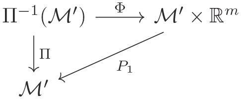
The fiber bundle approach of [33] for generalized Finsler spaces is general enough to encompass all aspects of the present description. In usual continuum mechanical settings, the reference configuration is identified with a particular instant in time at which a deformable solid body is considered undeformed. A differential manifold
Let
Define
2.1.1. Basis vectors and nonlinear connections
In (generalized) Finsler geometry, coordinate transformations from

where


Similarly, for the holonomic basis on


Clearly, the

By construction [35],

The set

The

The horizontal subspace is thus not involutive unless (2.9) vanishes identically, and
Subsequent presentation assumes vertical and horizontal subspaces of the same dimension:

Specialization in (2.10) is standard in Finsler geometry [29, 33] and not overly restrictive for subsequent applications. A formal way of achieving (2.10) using soldering forms is given in [35], whereby
Finally, coordinate differentiation operations are denoted by the following condensed notation:

2.1.2. Metric tensors, lengths, areas, and volumes
The Sasaki metric tensor [29, 36, 67], symmetric by definition, enables a natural inner product of vectors over


Components of
Let

The scalar volume element and the volume form of

The second of definitions (2.15) is consistent with [39]; others exist [68, 69], e.g., those representing volume elements and forms on total space

2.1.3. Linear connections and covariant derivatives
Let ∇ denote the covariant derivative. Horizontal gradients of basis vectors are determined by generic affine connection coefficients

Vertical gradients are specified by generic connection coefficients

As in a prior example, let
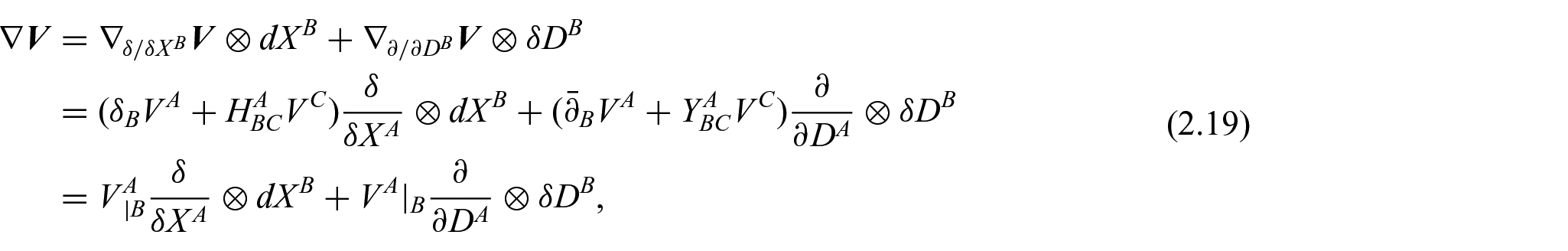
where

The following identity is also noted for

Particular linear connections used often in Finsler geometry are discussed next. Christoffel symbols of the second kind for the Levi-Civita connection on

Cartan’s tensor is defined as

Horizontal coefficients of the Chern–Rund and Cartan connections are defined as

Finally, the Berwald linear connection coefficients are defined on

Individually, (2.22), (2.23), and (2.24) are torsion-free, i.e., symmetric. The Chern–Rund–Cartan connection coefficients are metric-compatible for horizontal covariant differentiation of

Then
With the metric tensor now introduced, different sets of nonlinear connection coefficients

Let

For characterization purposes, let
2.1.4. Stokes’ theorem on the base manifold
Let


where
First, the integrand on the right of (2.30), i.e., the
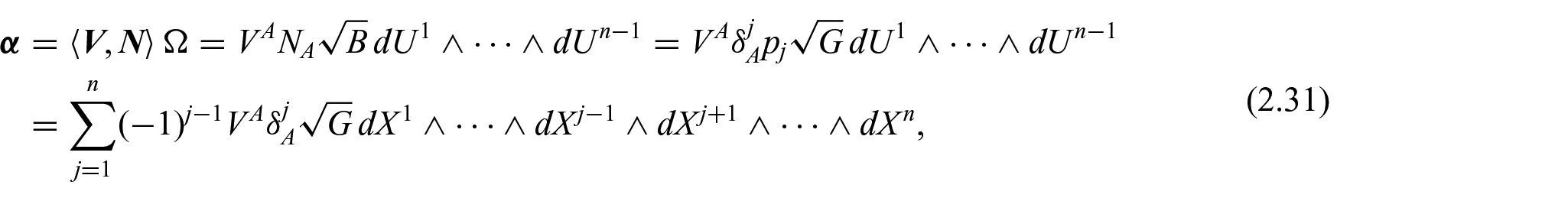
where
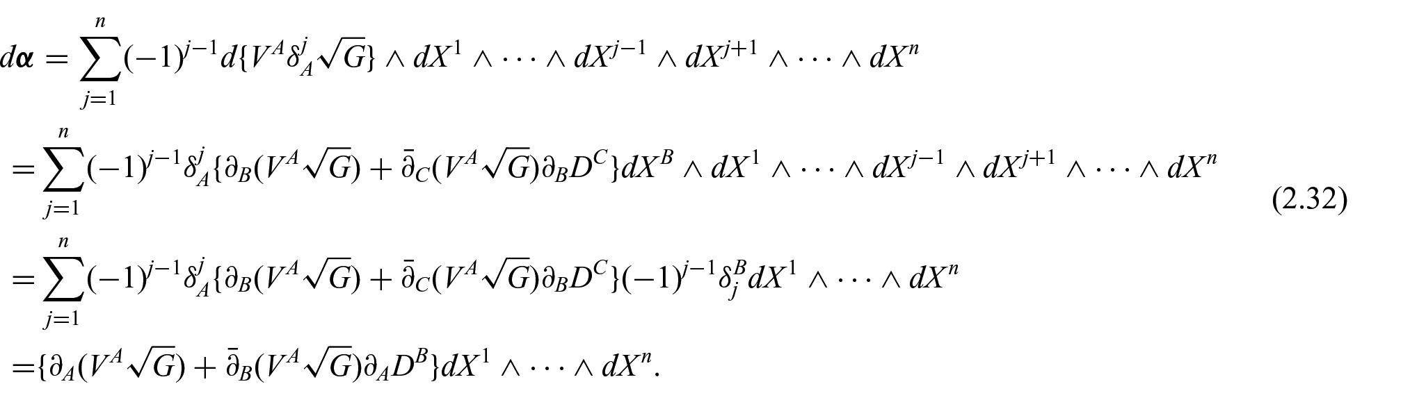
Using (2.21) with

and then using the first of (2.26),

Then noting that

where condensed notation is
2.1.5. Pseudo-Finsler and Finsler spaces
Developments to this point apply for generalized Finlser geometry, wherein the metric tensor components need not be derived from a Lagrangian [33, 37, 38]. Particular subclasses of generalized Finsler geometry require such a Lagrangian function, denoted by
Let

is non-singular over

In Finsler geometry [28, 29, 33], it follows that

2.1.6. Reductions and embeddings
A (strict)
Fn → Mn, where
Fn → Vn, where
Fn → En, where
Notions regarding embeddings of Finsler spaces in Riemannian spaces are summarized from [28, 73, 74]:
a Finsler space
a Finsler space
a Finsler space
2.2. Spatial representation via a fiber bundle
An analogous description on a fiber bundle is used for the spatial, i.e., current, configuration of a body. A differential manifold
The global mapping from referential to spatial base manifolds is
Definitions in the remainder of Section 2.2 fully parallel those of Section 2.1, where lowercase indices and symbols, with the exception of connections, are used to distinguish current-configurational quantities.
2.2.1. Basis vectors and nonlinear connections
Coordinate transformations from

where

The set


Subsequently, take

Spatial coordinate differentiation is described by the compact notation

2.2.2. Metric tensors, lengths, areas, and volumes
The Sasaki metric tensor [67] providing an inner product of vectors over


Let

The scalar volume element and volume form of

The embedding of an

2.2.3. Linear connections and covariant derivatives
Let ∇ denote the covariant derivative. Horizontal gradients of basis vectors are determined by generic affine connection coefficients


Let
Operations


The Berwald linear connection on

2.2.4. Stokes’ theorem on the base manifold
Let

where
2.2.5. Pseudo-Finsler and Finsler spaces
Definitions in Section 2.1.5 carry over directly from
2.2.6. Reductions and embeddings
Remarks in Section 2.1.6 transfer directly to the spatial representation.
3. Historical applications in field theory and mechanics of continua
The potential utility of Finsler geometry for continuum mechanics applications was recognized by several prominent theoreticians of the mid-twentieth century. Kondo [75] posited trial ideas towards a yielding criterion for plasticity based on deviations from geodesics of a Finsler space with a curvature tensor derived from the Chern–Rund–Cartan horizontal connection coefficients
However, none of the aforementioned researchers (i.e., Kondo, Kröner, nor Eringen) appear to have developed a continuum mechanical theory, i.e., a description of kinematics and balance laws of continuous bodies, based on Finsler geometry. Rather, the first continuum mechanical theory with a basis in Finlser geometry is apparently due to Amari [31], dealing with elastic–plastic–ferromagnetic crystals. Generalized Finsler-type treatments of solid bodies, with a focus on kinematics, were subsequently formulated by Ikeda [77] and Bejancu [33]. Key features of each of these works [33, 63, 77] are reviewed in what follows next. Choices of metric tensors, connection coefficients, motions, and tangent mappings between material and spatial configurations are highlighted in each case. None of these works contain solutions to any boundary value problems; hence, predictive capabilities of these early theories cannot be fully evaluated.
3.1. Amari’s theory of mechanics of ferromagnetic substances
The first theory (known to the present author) describing geometry, kinematics, and balance laws of solid mechanics with a basis in Finsler geometry is due to Amari [63]. The general kinematical theory admits finite deformation; however, derivations of balance laws invoke geometric linearization. A spatial, rather than material, description is adopted for implementation of Finsler concepts.
3.1.1. Geometry and kinematics
The geometric formalism of Section 2.2 of the present work applies to Amari’s theory, albeit with several extensions. The base manifold
Vector field

Such an immersion is not possible, in contrast, for the total generalized Finsler space
A reference configuration in the form of a generalized Finsler bundle, as in Section 2.1, is not introduced in the theory of [63]. Rather, a locally unloaded or relaxed configuration of the crystal (Figure 1), with base space denoted by

where

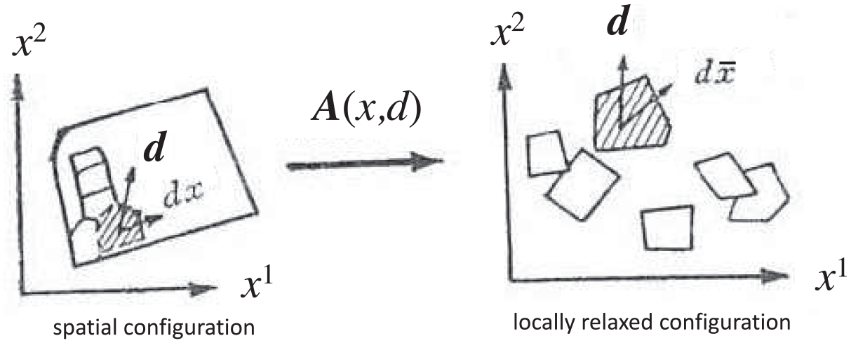
Ferromagnetic crystalline solid in spatial configuration (left) and locally relaxed, natural configuration (right), based on Figure 3 of [63]. The spin direction vector
In analogy to the elastic–plastic decomposition of deformation gradient
The spatial metric components

The spatial metric is expanded in (even) powers of

where the fourth-order tensor of magnetostriction constants is

where
No nonlinear connection

For a generalized Finsler space with distant parallelism, affine connections are prescribed as

This connection has non-vanishing torsion tensors, but it is metric compatible with
Other specializations of the geometric theory explored in [63] include reduction to an osculating non-Riemannian space, whereby
3.1.2. Equilibrium conditions
Balance laws of momentum conservation are derived in [63] under the conditions of small deformations and additive separation of lattice displacement gradient:


Elastic lattice distortion is

Total potential energy density depends on displacement
Euler–Lagrange equations are obtained from a variational principle with independent variations

The variational principle of [63] is as follows, where

with

a macroscopic balance of angular momentum consisting of three independent PDEs because

and a microscopic force balance in the spin domain, consisting of three PDEs subject to constraint (3.1),

Free natural boundary conditions on

A particular form of energy density
In a subsequent refinement of the theory in [63], a different covariant differential and corresponding modified connection coefficients have been suggested [79] such that the Euclidean length of the directors given by
3.2. Ikeda’s theory of directors in the mechanics of oriented media
Similarly to the fiber bundle approach in Section 2, denote by
Let

Components of the deformation gradient

The following transformations are posited in [77]:

with
The external derivative of the second of (3.20) is calculated as [77]

where

with

implying
The treatment of the spatial configuration in [77], in contrast to the reference configuration, admits a generalized nonlinear connection. Dual basis vectors on

The covariant derivative of a spatial vector field of components
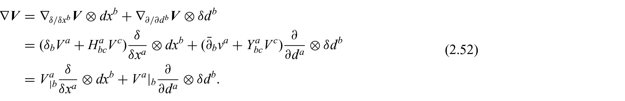
This expression reduces to (2.52) when
Let

To complete the geometric description, connection coefficients
3.3. Bejancu’s theory of geometry and deformations of oriented media
Another rather early application of Finsler geometry towards finite deformation of solid bodies comprises Chapter 8 of the monograph [33]. Fiber bundle descriptions of Sections 2.1 and 2.2 for
Recall from Section 2.1 that coordinate fields on

Components of the deformation gradient and its inverse are, as in (3.19),

Holonomic basis vectors

Accordingly, “deformed” nonlinear connection coefficients

As derived in [33] under assumptions inherent in (3.27)–(3.30), linear connection coefficients are pushed forward from reference ((2.17) and (2.18)) to current ((2.50) and (2.51)) configurations through deformation


Convected covariant metric tensor components for

When
4. Contemporary applications in nonlinear mechanics and materials physics
Applications of generalized Finsler geometry to continuum mechanical problems remain scarce. Using a pseudo-Finsler fiber bundle approach similar to that outlined in [33] and Section 3.3, the theory of [82] associates
The first known application of generalized Finsler geometry to calculate a material response in the context of mechanics of solids with microstructure was reported in the monograph [87], and more concisely summarized in [68, 88] with extensions in [89, 90]. In that work, reviewed in detail in Section 4.1, a complete continuum mechanical theory was developed, and the constitutive response was calculated numerically for a polycrystalline bar element undergoing combinations of homogeneous extension and shear. A more recently developed, complete theory of generalized Finsler-geometric continuum mechanics, originally published in [61, 91], contains the first known (semi-)analytical solutions to equilibrium equations for boundary value problems using a model of this class. Further theoretical advancements and solutions to many other physical problems, both analytical and numerical, were reported in [62, 72, 92–96]. Ideas from this body of work are reviewed in Section 4.2. New example problems in Section 4.2 demonstrate features of model predictions for a material body framed in generalized Finsler space absent for a material body framed in Euclidean space. Several improvements that alleviate inessential assumptions in the original framework [61, 91] are newly advocated.
4.1. Saczuk’s generalized Finsler theory of oriented media
Saczuk et al. [68, 87–90] invoked Finsler geometry to construct finite-deformation mechanics models of solids with microstructure. Director
4.1.1. Governing equations
The generalized fiber bundle-type description of reference and current configurations of a material body given in Sections 2 and 3 applies. Recall that

supplies the matching Sasaki metric tensor components
Coordinates of material points

where

In component form, horizontal


Mixed-configurational components of linear connections are attained by shifting

where it is assumed that deformations of line elements obey

Lagrangian strain tensors

Differences between squared total line lengths follow from (4.6)–(4.8) as

Balance laws were postulated as follows in [68, 87, 88], restricting current attention to the quasi-static, isothermal, and non-dissipative case. A Lagrangian function

with

where a similar description of

with
The local macroscopic linear momentum balance is the following, with

The double summation on components of

Traction boundary conditions on

with

these are perfectly analogous to those of classical continuum mechanics [2, 45], whereby corresponding Cauchy stress(es) are symmetric. Rate dependence, temperature, and dissipation were also discussed in [68, 90]; details are beyond the scope of this review. Furthermore, extensions to address viscoelasticity, damage mechanics, and gradients of
4.1.2. Material response problem
In the earliest known application of Finsler geometry to predict a material response in the context of mechanics of solids with microstructure, Saczuk [87] and Stumpf and Saczuk [68] used the quasi-static theory reviewed in Section 4.1.1 to study deformation of a material element representative of a bar loaded in tension and/or shear, with

More specifically,

Heuristic arguments were given in [68, 87] that associate
A single material element corresponding to a bar of length

where
At each increment, the metric tensor, deformation gradient, linear and nonlinear connection coefficients, strain measures, and stresses are calculated. The stress fields so obtained should satisfy (4.13)–(4.16). Whether this consistency is simply assumed, or if the governing PDEs with boundary conditions are solved numerically, is unclear from the text [68, 87].
Computed results show features qualitatively similar to those of polycrystalline metals undergoing strain softening. Even though the free energy density
4.2. Finsler-geometric continuum mechanics
The present author used concepts from generalized Finsler geometry to construct a complete variational theory for nonlinear elastic bodies with microstructure. The original theory [61, 91] accounts for finite deformations under conditions of static equilibrium for forces conjugate to material particle motion and state vector evolution. Time dependence does enter this theory, which is reviewed in Sections 4.2.1–4.2.3, with several demonstrative problems solved in Section 4.2.4. Extensions to explicit time dependence, dynamics, and dissipative processes are noted in Section 4.2.5.
4.2.1. Motions and deformations
Particle motion

with

Note that the fiber dimensions are chosen as
From (4.20) and (4.21), the following transformation formulae apply for partial differentiation operations between configurations of a differentiable function

However, unlike the theory of [33] reviewed in Section 3.3, basis vectors need not convect from

meaning
As implied in (4.23), the deformation gradient field

The inverse deformation gradient

Usual stipulations on regularity [3] of motions (4.20) apply such that
Transformation equations relating differential line elements of (2.14) and (2.47) follow as

Applying (4.26), definitions of the determinant, and (2.15) and (2.48), volume elements and volume forms, respectively, transform between reference and spatial coordinate systems on


Lengths of deformed and initial line elements can be compared using the Lagrangian deformation tensor

It follows that

A similar procedure with the second of (2.50) yields
4.2.2. Pragmatic assumptions
Stokes’ theorem 1 and (2.30), which extends the divergence theorem of Rund [39] to the base manifold

where the second of (4.31) is implied by the first under a consistent change of variables. Existence of the following functional forms emerges from (4.20), (4.21), and (4.31):


These functional forms are not inconsistent with (4.20): if functions (4.31) are known, then
The present theory, similar to those in [63, 68, 87], does not require that

where
Another requirement for use of (2.30) for arbitrary admissible

If metric

while the preferred choice of nonlinear connection
Once the field of referential generalized Finsler metric components
The following decomposition of

It proves convenient to choose
Statements of the prior paragraph for
4.2.3. Energy functional and static equilibrium equations
A variational principle is invoked, where

Surface forces are

where the variation of
Independent variables entering
Expansion of the integrand on the left-hand side of (4.38) is written

Here


Choices of connection coefficients in (4.34) and (4.35) are invoked, noting
The culminating Euler–Lagrange equations consist of the macroscopic balance of linear momentum:

and the balance of micro-momentum (i.e., director momentum or internal state equilibrium):

The natural boundary conditions derived on

Imposition of invariance under rigid rotations of spatial coordinate frames leads to the restricted form of energy density:

from which the first Piola–Kirchhoff stress

Given natural boundary conditions (4.44) and/or essential boundary conditions (prescribed
4.2.4. Simple example problems
One-dimensional (1D) problems on base manifold
Herein,
The formulation of Sections 4.2.2 and 4.2.3 reduces as follows for the 1D case. Spatial coordinates are

Noting that

However, the Cartan tensor

The pertinent component of deformation gradient and horizontal director gradient are, respectively,

The deformation tensor has axial component

The value of
Energy density entering (4.37) and (4.45) is specialized as follows, noting

Function
Macroscopic and microscopic stresses are

Macroscopic linear momentum balance (4.42) reduces to

where

Here,

Let

where

where
Summarizing, fracture prescriptions are

where parameter

Microscopic momentum balance (4.58) is then

Non-zero
Two specific boundary value problems are solved. The first invokes boundary conditions at

Sought are solutions of the form

Balance (4.61), with

For tensile loading, the positive root applies. Solutions for
Solutions derived in (4.63) and (4.64) are given in Figure 2, with total energy and domain length with respect to

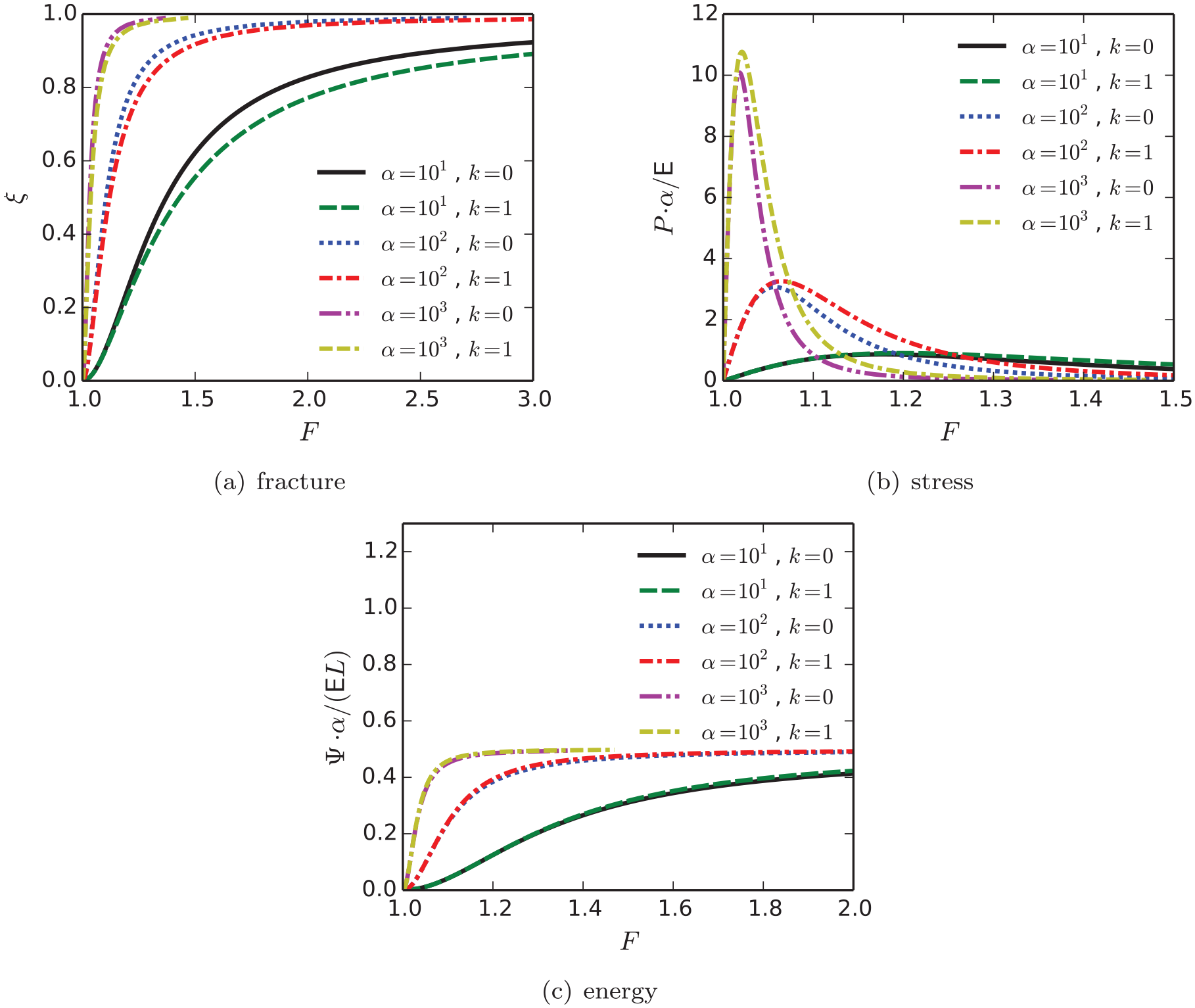
Solutions to homogeneous fracture problem (4.64) for Finsler (
Solutions to stress-free fracture problem (4.67) for Finsler (
As
The second fracture problem models complete fracture at

Stress-free conditions require, from (4.60),

For Riemmannian geometry (
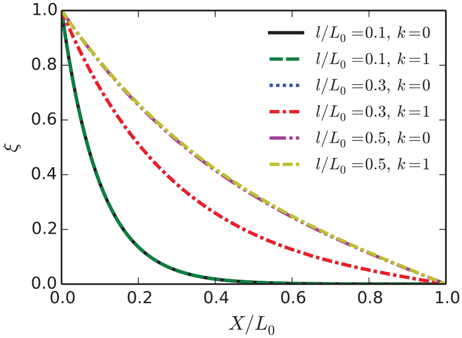
Profiles of

where
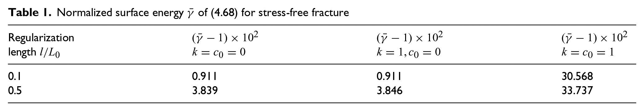
Normalized surface energy
The eigenstrain for intermediate states

Define

A logarithmic nonlinear elastic potential
Summarizing the above modeling assumptions, phase transformation prescriptions are

where parameter

Microscopic momentum balance (4.58) is, with

As was the case for the fracture example, non-zero
One specific boundary value problem is solved, with boundary conditions at

Homogeneous solutions of the form

Microscopic balance (4.73) becomes, with

A closed-form solution for
The transformation strain is chosen as

From Figure 4(a), as
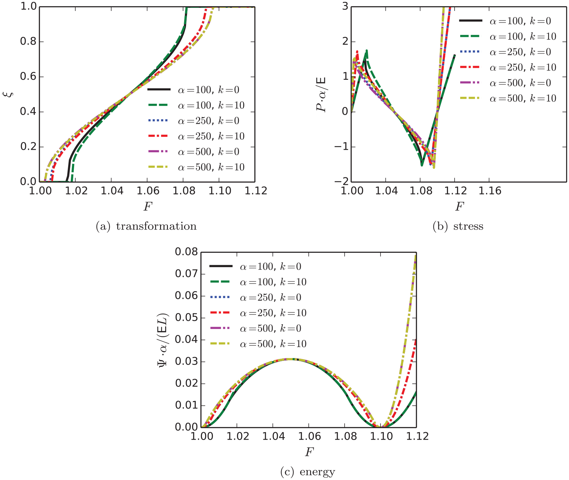
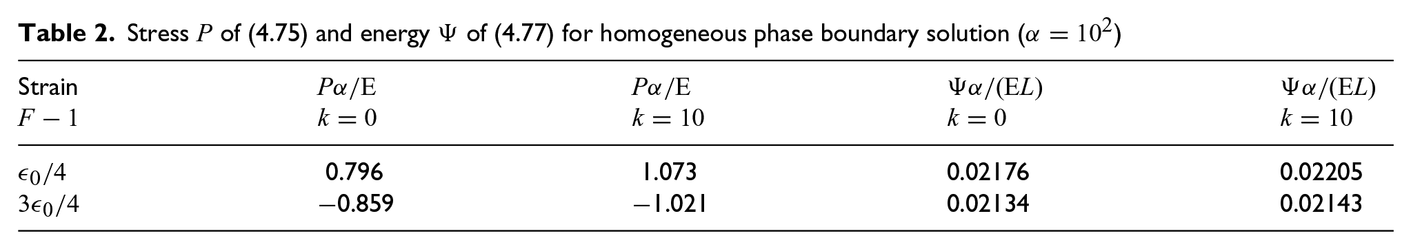
Homogeneous phase change solutions of (4.76) for Finsler (
Note from Figure 4(c) that energy attains a local maximum at
Stress
4.2.5. Extensions and applications
Recent advances in Finsler-geometric continuum theory consider the following:
Nonlinear elastic bodies undergoing shear failure, with
Additive or multiplicative decompositions [5, 63] of
Multiplicative decompositions of
Boundary value problems for simultaneous torsion, axial stretch, and/or radial contraction, with time-dependent field
Numerical simulations of polycrystals with
Fully dynamic fields
A transport theorem and jump conditions for mass, momentum, and energy exchange across a moving planar surface of discontinuity are derived in [72, 96]. Solutions to the jump conditions are obtained for crystals under shock compression undergoing shear on pyramidal planes [72, 95, 96].
Problems solved in [61, 62, 72, 92–96] have considered various crystalline materials (e.g., ice, metals, ceramics) with realistic properties and comparison with experiments and/or quantum mechanical results.
5. Ferromagnetic crystals revisited
In this final section, the generalized Finsler-geometric theory of Section 2 (mathematical foundations) and Section 4.2 (variational continuum mechanics) is adapted to describe ferromagnetic materials, revisiting a topic addressed by the apparent first continuum mechanical theory based on Finsler geometry [63]. The present theory essentially extends the nonlinear quasi-magnetostatic theory of Maugin and Eringen [64, 110] from its original setting on a Riemannian (and, more specifically, Eucildean) material manifold to a generalized Finsler manifold
Notable differences between the present approach and that of Amari [63] reviewed in Section 3.1 are as follows:
lattice deformations
finite deformations are considered in the variational formulation, unlike the linearized treatment in Section 3.1.2;
a spatial-rotationally objective constitutive theory is constructed, unlike the formulation of Section 3.1.2 that includes explicit potential energy dependence on lattice rotations and lattice rotation gradients;
the divergence theorem for generalized Finsler space, (2.30) of Theorem 1, is used to derive local equilibrium equations, unlike the treatment of Section 3.1.2 that invokes the classical divergence theorem on Euclidean space with a Cartesian metric;
the director vector of Finsler geometry is of constant magnitude with respect to an Euclidean metric, but it is not necessarily of unit length as in Section 3.1;
a different, and more general, form of Finsler metric is admitted in the present theory to capture various interactions between the magnetization direction and atomic-scale structure, as opposed to that of Section 3.1.1 accounting only for magnetostriction.
Fundamental aspects of this new theory of Finsler-geometric continuum mechanics of magnetically saturated, nonlinear elastic solids are defined and derived in Sections 5.1–5.5. A representative generalized Finsler metric, with conceivable physical origin, is chosen in Section 5.6 to demonstrate resulting differences from the original theory based in Euclidean space [64, 110].
5.1. Director vectors and fiber coordinates
The director vector field

Covariant components
Fiber coordinates on

Clearly,

Subsequent calculations are vastly simplified if connection coefficients for horizontal gradients of basis vectors on

Analogous spatial horizontal covariant derivatives

Consequences of the constant magnitude constraints in (5.1) and (5.2) with (5.4) include

Similar constraints are derived as follows for a variational differential

As

5.2. Energy density and variational principle
A local energy density

Dependence on deformation gradient
Let

Here,

Following [64], the following variational principle is posited, here in the absence of macroscopic mechanical inertia:

The left-hand side of (5.12) accounts for the change in stored energy of the body subject to the constraint that

where

Reference mass density is

5.3. Euler–Lagrange equations and electromechanical boundary conditions
Equations (5.10), (5.11), and (5.13)–(5.15) are substituted into (5.12). Theorem 1, i.e., (2.30), is used with integration by parts to convert volume to surface integrals. Independent variations are
Assuming (5.12) must hold for all admissible variations

Expression (5.16) is identical to (4.42) with the exception of body force contributions. Natural mechanical boundary conditions obtained

The remaining terms in volume integrals from (5.12), localized to a point

which is a microscopic work balance. Applying (5.8) to eliminate

As

Finally, natural boundary conditions for the electronic spin continuum are derived from (5.12) and (5.13) as follows, in agreement with (4.44) and [44]:

5.4. Objectivity and macroscopic angular momentum
Energy density

Here the field variables

Note the symmetries
The spatial Sasaki metric

This is analogous to the decomposition of
The set of 15 quantities

From (5.10) and (5.23), the thermodynamic force

The micro-stress

First Piola–Kirchhoff stress

Recall from (4.46) that the Cauchy stress tensor is

The term

None of
5.5. Maxwell’s equations and electromagnetic boundary conditions
Local versions of Maxwell’s equations for non-polar continua in the magnetostatic approximation (i.e., no electric field, electric current, or electric polarization) are

Denoted by

5.6 Example metric with reduced governing equations
A particular, relatively simple, example is used to highlight differences between the generalized Finsler model of ferromagnetic solids formulated in Sections 5.1–5.5 and the theory of [64, 110] framed in Euclidean space.
5.6.1. Coordinates and metrics
Respective sets of Cartesian coordinates

Here,
5.6.2. Connection coefficients
Recall from Section 4.2.2 that vertical affine coefficients of the Chern–Rund connection vanish by definition, and from Section 5.1 that horizontal gradients of basis vectors on fiber spaces vanish. For convenience, take referential holonomic basis vectors on

Coefficients

In contrast, Cartan tensors (2.23) and (2.54) do not always vanish since metrics


noting
5.6.3. Reduced governing equations
Applying (5.5) and (5.33)–(5.37) to (5.16), (5.30), (5.20), and (5.31), reduced forms of the macroscopic balance of linear momentum, macroscopic balance of angular momentum, balance of electronic spin momentum, and Maxwell’s equations are obtained, respectively:


Left-hand sides of each equation in (5.38)–(5.41) agree with [64, 110]. Non-vanishing terms on right-hand sides of (5.38) and (5.40) are the only differences from the theory of [64, 110] for the macroscopically quasi-static case with spin inertia. When
5.6.4. Magneto-elastic energy and Finsler metric scaling
The model is complete upon specification of energy density
The key new contribution of the present theory is implementation of

Consider first a cubic ferromagnetic crystal with lattice directions [100], [010], [001] aligned parallel to

Dimensionless material constants

where


Thus, for prescription (5.43) of a cubic crystal, all balance laws revert to those of Riemannian geometry.
Finally, consider a uniaxial (e.g., hexagonal) ferromagnetic crystal with c-axis [0001] oriented along


Finsler-originated contributions on the right-hand sides of (5.49) and (5.50) (
6. Concluding remarks
Early and contemporary theories of continuum mechanics of solids with foundations in generalized Finsler geometry have been analyzed. A modern theory of Finsler-geometric continuum mechanics has been refined, with new analytical and numerical solutions reported for 1D problems involving fractures and phase transformations. The modern theory has also been newly adapted to model ferromagnetic solids in the magnetically saturated state. Differences among governing equations, and problem solutions where applicable, among theories based in Finsler space versus those based in affine Riemannian space have been highlighted. Results demonstrate how the Finsler approach might enrich descriptions of physical phenomena, requiring, minimally, only a single additional parameter entering Sasaki metric tensors.