Dynamics of a string subjected to a dual-point contact moving mass

Abstract

This study investigates the planar transient dynamics of a linearized string interacting with a moving mass. Unlike conventional models that idealize the moving system as a point mass or particle, the mass is modeled more realistically as a finite body that maintains dual contact with the string at closely spaced points. This modeling choice naturally incorporates the rotational inertia of the moving mass into the formulation. For a prescribed motion of the moving mass along the string, the coupled governing equations are derived in terms of the Dirac delta function. In the limiting case where the two contact points approach at the mass center, the formulation reduces to an equivalent monopole–dipole representation. The governing equations are discretized using the Galerkin method and integrated in time via a Runge–Kutta scheme. The formulation is first applied to a stretched string subjected to a uniformly moving mass. Particular attention is given to the trajectory paradox reported in earlier studies for moving point masses near a boundary. Using the present two-point contact model, this paradox is examined in terms of trajectory at the front contact, the separation between the actual and virtual centers of mass, and the variation in contact-point spacing induced by abrupt responses near the boundary. Subsequently, a new system, in which a string is vertically hung and carries a uniformly moving mass, is analyzed. Trajectory convergence is demonstrated for both ascending and descending motions. Similar to the trajectory paradox, a jump-like response appears near the upper fixed boundary when the mass ascends at higher velocities. At these velocities, the two-point contact model yields divergent results across the entire domain, indicating limitations in its applicability. This behavior highlights the need for future studies that incorporate nonlinear effects to more accurately capture the observed dynamics.

Keywords

moving mass string dynamics moving two-axle system trajectory paradox hanging string

1. Introduction

In mechanics, particularly in structural and transportation engineering, loads that change with position and time are referred to as moving loads. The study of moving loads on structures has been an area of research since the advent of motorized transportation. This field has numerous engineering applications, including vehicles traveling over bridges, cable cars on ropeways, overhead cranes, trains on railway tracks, fighter jets on aircraft carrier decks, conveyor systems, and high-speed pods in hyperloop systems. Unlike stationary loads, moving loads introduce complexities such as transient vibrations, resonance phenomena, and unusual displacements, making the analysis mathematically rich and practically challenging.

Over the years, researchers have refined their models of moving systems to better understand how structures respond to loads traveling across them. The simplest model is a moving point force [1 –4], which represents the load as a single concentrated force moving along the structure. This approach is valid when the moving system is significantly smaller than the structure, and its inertial effects are negligible. When the transverse inertia of the moving system cannot be ignored, the model is upgraded to a moving point mass (or particle) [5 –12]. If we further include the system’s own stiffness, damping, and inertia, along with how these properties interact with the structure, the model becomes a moving oscillator [4,13 –15].

In addition, researchers have examined a wide range of non-point moving loads, including moving trains of forces or continuous moving masses [16 –18], two-axle [19 –22] and multi-axle systems [23,24], distributed and patch (area) loads, vehicle models with multiple degrees of freedom, finite-length loads with either uniform or variable characteristics, and loads with varying intensities. A comprehensive overview of these formulations is provided by Frỳba [4], who systematically analyzes and solves various types of moving-load problems on different structures. Bajer and Dyniewicz [25] have also addressed moving-mass problems on various structures using multiple approaches, including analytical, semi-analytical, numerical methods, the Newmark method, and space–time finite-element techniques.

Various studies have been conducted on one-dimensional structures with a moving point mass, such as a beam and a stretched string. In the mid-19th century, Willis [26] presented one of the earliest analyses of beams subjected to moving loads. Alongside developing an approximate theoretical solution, he conducted experiments to compare the responses of beams under static and dynamic loading. Shortly after, Stokes [27] provided an exact solution for a simply supported Euler–Bernoulli beam carrying a moving mass. His formulation included the inertia of the travelling particle and examined limiting cases, such as neglecting the beam mass relative to the moving load. The solution revealed an interesting behavior: as the mass approached the right support, its predicted vertical position did not approach zero, contrary to what would be expected for a simply supported boundary. This anomaly became one of the notable insights into the complexities of moving-mass problems.

Nearly a century later, Smith [5] revisited the moving mass problem, this time examining a horizontal, stretched string instead of a simply supported beam. His finding was similar to what was earlier reported by Stokes, that as the mass approached the terminating end of the string, its predicted position exhibited a discontinuity, terminating at a point different from the expected taut boundary. Dyniewicz and Bajer [6] examined the trajectory paradox by approximating the transverse displacement using a truncated Fourier sine integral series. They report similar behavior for an inertial string.

In recent years, the trajectory paradox for a moving point mass on a stretched string has been resolved in a series of studies [7,28,29] employing geometrically nonlinear string model that account for the coupling between transverse and longitudinal motions. Gavrilov et al. [7] revisited this long-standing problem by incorporating both geometrically nonlinear string model and wave-pressure effects, and examined their influence on the dynamics of the moving mass. Ferretti et al. [28] derived the governing equations for a mass moving along a stretched string and analyzed a reduced-order model using the Galerkin method. This study captures axial effects through tension variation. In a subsequent study, Ferretti et al. [29] further extended this framework by explicitly including dynamic tension due to axial stretching, referring to the resulting boundary irregularity as the Stokes–Smith paradox and investigating its convergence behavior along with the associated axial motion of the string.

Previous studies on the trajectory paradox have primarily modeled a point mass moving on a stretched string. In contrast, the moving system has not been treated as a two-axle or dual-point contact system on a stretched string, despite such models being widely used in beam dynamics. One of the earliest related contributions is by Wen [22], who introduced a two-axle model for moving vehicles on beams rather than a continuously distributed moving load. His results highlighted the significant influence of axle separation on the dynamic response. Subsequently, Frỳba [4,20] investigated how system parameters affect vibration characteristics. Additional studies on beams subjected to moving two-point contact loads include [19,30 –34]. For stretched strings, the effect of rotary inertia of a moving mass was considered more recently by Kumar and Gupta [9], who showed that the magnitude of the trajectory jump is largely insensitive to rotary inertia. This configuration can be regarded as a limiting case of a two-point contact system when the separation between the contact points approaches zero at the midpoint.

To the best of the authors’ knowledge, existing studies on moving-mass problems primarily focus on stretched strings [5,6,29] or slack catenary strings [35,36] subjected to a moving mass. However, the dynamic response of a hanging string under a moving mass remains largely unexplored. Such configurations arise in several engineering applications, including structural systems, industrial robotics, and the control of robotic manipulators. Representative examples include fast-roping operations in military deployments, where the motion of a descending soldier influences the system’s dynamic behavior, and rope-climbing robots. These robots are increasingly employed in high-altitude and hazardous tasks such as sluice maintenance, bridge inspection, high-rise building cleaning, and rescue operations [37,38]. Studies related to hanging strings have primarily considered configurations with a fixed tip mass [39 –42], in which the string tension varies along its length. For a hanging string with a moving mass, the tension varies both spatially and temporally. Moreover, the asymmetric boundary conditions (fixed at the top and free at the bottom) introduce additional complexity, leading to rich and nontrivial dynamic behavior.

In this study, these gaps in the literature are addressed by developing a general formulation for a linearized string subjected to a moving mass with two-point contact. Two specific systems are then investigated. First, the influence of the two-point contact model on the trajectory paradox, previously reported for a moving point mass on a stretched string, is examined. Subsequently, the dynamics of a linearized hanging string carrying a uniformly moving mass are analyzed for both ascending and descending scenarios.

This paper is organized as follows. Section 2 presents a general mathematical formulation for a prescribed moving dual-point contact mass traveling on a linearized string. The governing equation is derived using Dirac delta functions and is shown to reduce to a monopole–dipole representation under an appropriate limiting condition. In Section 3, the governing equations are non-dimensionalized to reduce the number of effective parameters and obtain a simplified formulation. Section 4 applies the Galerkin method to discretize the system, leading to a reduced matrix equation expressed in modal coordinates. The proposed formulation is then applied to two representative problems: a stretched string with a moving mass in Section 5, and a hanging string carrying a moving mass in Section 6. Finally, conclusions are drawn in Section 7.

2. Mathematical modeling

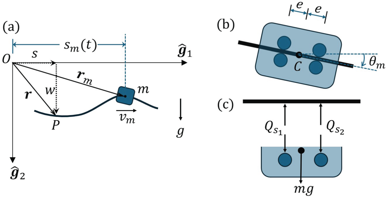
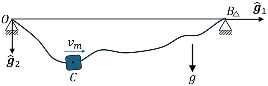
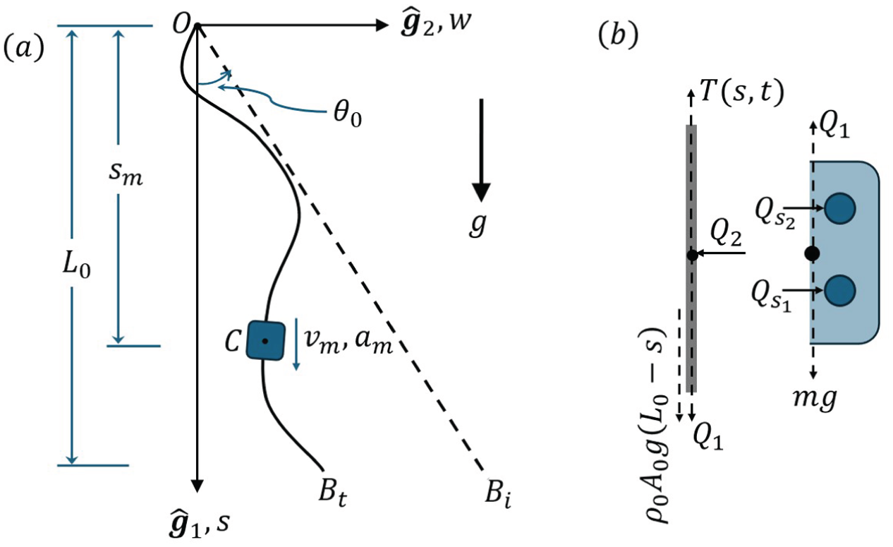
Figure 1(a) illustrates a schematic of a linearized string element carrying a moving mass in a plane. A fixed right-handed orthonormal Cartesian frame (RHOCF) $(\tilde{G}, O, {\hat{g}}_{j})$ , with $j \in 1, 2$ , is introduced to define the coordinate system and kinematics. The material coordinate s parametrizes the undeformed length of the string, while $w (s, t)$ denotes the transverse displacement of a material point at time t, measured along ${\hat{g}}_{2}$ . Gravity acts in the ${\hat{g}}_{2}$ direction, and the equilibrium configuration of the string is assumed to be straight along ${\hat{g}}_{1}$ . Dynamic axial displacement in the string is neglected. The string is characterized by a uniform mass density $ρ_{0}$ , constant cross-sectional area $A_{0}$ , and undeformed length $L_{0}$ . The material is assumed to be linearly elastic, homogeneous, and isotropic.

Figure 1.

(a) A linearized string element interacting with a moving mass that travels with a prescribed velocity $v_{m}$ along the ${\hat{g}}_{1}$ direction. Gravity acts in the ${\hat{g}}_{2}$ direction. (b) The moving mass is connected to the string through two point contacts, each located at an eccentric distance e from the mass center. (c) The free body diagram (FBD) of the moving mass and also illustrates the transverse reaction forces exerted at the two contact points on the string.

The position vector of a material point P on the string, see Figure 1(a), at time t, can be written as follows:

\begin{matrix} r (s, t) = s {\hat{g}}_{1} + w (s, t) {\hat{g}}_{2} . \end{matrix}

(1)

The moving mass of magnitude m, modeled as a cable-climbing robot with dual-point contact, engages the string at two discrete contact locations, as shown in Figure 1(b). This moving mass is similar to a two-axle moving system on a beam considered in [20 –22]. Unlike conventional moving systems (such as vehicles) on horizontal beams, which may operate with a single wheel at each contact point, the present system requires two wheels at each contact to securely grip the string. The center of mass lies midway between these contact points at point C. The mass is assumed to have finite rotary inertia about its center of mass, given by

\begin{matrix} I = m {(μe)}^{2}, \end{matrix}

(2)

where e denotes the eccentric distance of each contact point from the center of mass. The parameter e is taken as the radius of gyration, while μ is the factor of gyration that characterizes the distribution of mass relative to the center. The factor μ satisfies $0 \leq μ \leq 1$ : $μ = 0$ corresponds to the case where all the mass is concentrated at the center, reducing the system to a moving point mass, whereas $μ = 1$ represents the limiting case in which the mass is entirely distributed at a distance e from the center. In the present model, the choice $μ = 1$ corresponds to two equal point masses of magnitude $m ∕ 2$ located at the two contact points.

For the system considered here, values of $μ > 1$ may also be admissible when the effective mass distribution extends beyond the distance e, which can occur for larger robots with relatively small contact spacing. The parameter e is referred to as the radius of gyration primarily for analytical convenience, as this definition simplifies the governing equations derived in the subsequent sections.

Furthermore, the moving mass is assumed to travel along the string with a prescribed, externally imposed motion $s_{m} (t)$ of its center of mass. Under the assumption of small transverse displacements, $s_{m} (t)$ also represents the instantaneous axial location of the mass center along the ${\hat{g}}_{1}$ direction. Assuming that the mass center remains coincident with the string (central line of the string), the position vector of the moving mass center can be expressed, using equation (1), as follows (see Figure 1(a)):

\begin{matrix} r_{m} (t) = r (s, t) |_{s = s_{m}} = r (s_{m}, t) = s_{m} {\hat{g}}_{1} + w (s, t) |_{s = s_{m}} {\hat{g}}_{2} . \end{matrix}

(3)

The above relation is expected to be valid for small transverse displacements and when the eccentricity e is much smaller than the string length, i.e. $e ≪ L_{0}$ . Accordingly, this study adopts a two-point contact model with closely spaced contact locations, representing a small two-axle robot that makes dual contact with a linearized string and possesses finite rotary inertia. The actual position vector $r_{C} (t)$ , or corresponding transverse displacement $w_{C} (t)$ , of the moving mass center is defined as the average of the position vectors and transverse displacements of the two contact points, respectively. Hence, sometimes in the result section, $r_{m} (t)$ will be referred to as the virtual center of mass position.

Taking total derivatives once and twice of equation (3) with respect to t, we get that the velocity and acceleration of the mass, respectively, as follows

\begin{matrix} {\overset{\cdot}{r}}_{m} (t) = v_{m} {\hat{g}}_{1} + ẇ (s_{m}, t) {\hat{g}}_{2} = ṡ_{m} {\hat{g}}_{1} + (ṡ_{m} w,_{s} + w,_{t}) |_{s = s_{m}} {\hat{g}}_{2}, \end{matrix}

(4)

\begin{matrix} {\overset{\cdot\cdot}{r}}_{m} (t) = a_{m} {\hat{g}}_{1} + ẅ (s_{m}, t) {\hat{g}}_{2} = {\overset{\cdot\cdot}{s}}_{m} {\hat{g}}_{1} + ({\overset{\cdot\cdot}{s}}_{m} w,_{s} + ṡ_{m}^{2} w,_{ss} + 2 ṡ_{m} w,_{st} + w,_{tt}) |_{s = s_{m}} {\hat{g}}_{2} . \end{matrix}

(5)

Throughout this work, $(□),_{a}$ represents the partial derivative with respect to variable a. $(\overset{\cdot}{□})$ represents total derivative with respect to time t, $(□^{'})$ represents total derivative with respect to position coordinate s, and $(□ |_{s = s_{m}})$ represents evaluation of an expression at $s = s_{m}$ .

In equations (4) and (5), $ẇ (s_{m}, t)$ and $ẅ (s_{m}, t)$ denote the transverse components of the velocity and acceleration of the moving mass, respectively. The transverse velocity $ẇ (s_{m}, t)$ contains two contributions: $ṡ_{m} w,_{s} |_{s = s_{m}}$ , which is the convective component arising from the motion of the mass relative to the string, and $w,_{t} |_{s = s_{m}}$ , which is the local (temporal) component associated with the time-varying deformation of the string.

Similarly, the transverse acceleration $ẅ (s_{m}, t)$ consists of four components. The term ${\overset{\cdot\cdot}{s}}_{m} w,_{s} |_{s = s_{m}}$ represents the convective contribution due to the relative acceleration of the mass; the term $ṡ_{m}^{2} w,_{ss} |_{s = s_{m}}$ is the convective contribution arising from the relative velocity; the term $2 ṡ_{m} w,_{st} |_{s = s_{m}}$ is a mixed, Coriolis-like component; and the term $w,_{tt} |_{s = s_{m}}$ corresponds to the local (temporal) acceleration of the string. Note that throughout this work, the analysis is restricted to uniformly moving masses, for which ${\overset{\cdot\cdot}{s}}_{m} = 0$ . Nevertheless, the formulation retains the contribution of the prescribed relative acceleration ${\overset{\cdot\cdot}{s}}_{m}$ to ensure generality and facilitate its application to future studies.

For a prescribed motion of the moving mass, its position $s_{m} = s_{m} (t)$ is known. Accordingly, the relative velocity $v_{m} : = ṡ_{m}$ and relative acceleration $a_{m} : = {\overset{\cdot\cdot}{s}}_{m}$ along ${\hat{g}}_{1}$ are also known. In contrast, the transverse displacement, velocity, and acceleration along ${\hat{g}}_{2}$ cannot be determined a priori, as they depend on the string deformation governed by the coupled dynamics of the string–moving mass system.

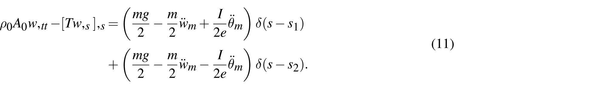
From Figure 1(c), the reaction forces $Q_{s_{1}}$ and $Q_{s_{2}}$ exerted by the moving mass act on the string in the negative ${\hat{g}}_{2}$ direction. Accounting for these transverse forces, the governing equation of motion for the string under a position-dependent tension $T (s)$ can be written as follows:

\begin{matrix} ρ_{0} A_{0} w,_{tt} - [Tw,_{s}],_{s} = - Q_{s_{1}} (t) δ (s - s_{1}) - Q_{s_{2}} (t) δ (s - s_{2}), \end{matrix}

(6)

where $δ (s - s_{j})$ represents a Dirac delta function and $s_{j}$ , for $j = 1, 2,$ is defined as

\begin{matrix} s_{1} = s_{m} (t) - e s_{2} = s_{m} (t) + e . \end{matrix}

(7)

From Figure 1(c), referring to the free body diagram (FBD) of the moving mass (robot), the linear momentum balance (LMB) along ${\hat{g}}_{2}$ and angular momentum balance (AMB) about C, respectively, are given as follows

\begin{matrix} mẅ (s_{m}, t) = mg + Q_{s_{1}} + Q_{s_{2}} \end{matrix}

(8)

\begin{matrix} I \overset{\cdot\cdot}{θ} (s_{m}, t) = e (Q_{s_{2}} - Q_{s_{1}}) . \end{matrix}

(9)

Inertial acceleration $ẅ (s_{m}, t) = ẅ_{m}$ is defined in equation (5). $θ (s_{m}, t) = θ_{m}$ , shown in Figure 1(b), is the orientation (rotation) of the mass and $\overset{\cdot\cdot}{θ} (s_{m}, t)$ is the corresponding angular inertial acceleration. Using equations (8) and (9), the reaction forces can be expressed as

\begin{matrix} Q_{s_{1}} = \frac{m}{2} ẅ_{m} - \frac{I}{2 e} {\overset{\cdot\cdot}{θ}}_{m} - \frac{mg}{2} and Q_{s_{2}} = \frac{m}{2} ẅ_{m} + \frac{I}{2 e} {\overset{\cdot\cdot}{θ}}_{m} - \frac{mg}{2} . \end{matrix}

(10)

Substituting these values into equation (6), we get

\begin{matrix} \begin{matrix} ρ_{0} A_{0} w,_{tt} - [Tw,_{s}],_{s} & = (\frac{mg}{2} - \frac{m}{2} ẅ_{m} + \frac{I}{2 e} {\overset{\cdot\cdot}{θ}}_{m}) δ (s - s_{1}) \\ + (\frac{mg}{2} - \frac{m}{2} ẅ_{m} - \frac{I}{2 e} {\overset{\cdot\cdot}{θ}}_{m}) δ (s - s_{2}) . \end{matrix} \end{matrix}

(11)

Now, the displacement compatibility relations at the two contacts can be written as

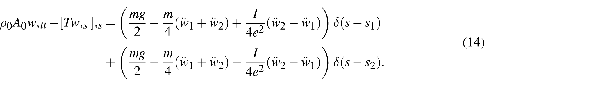
\begin{matrix} w_{1} = w (s_{1}, t) = w_{m} - e θ_{m} and w_{2} = w (s_{2}, t) = w_{m} + e θ_{m} . \end{matrix}

(12)

Here, $s_{1}$ and $s_{2}$ are substituted from equation (7). Taking total derivative of equation (12) twice with respect to t, we get

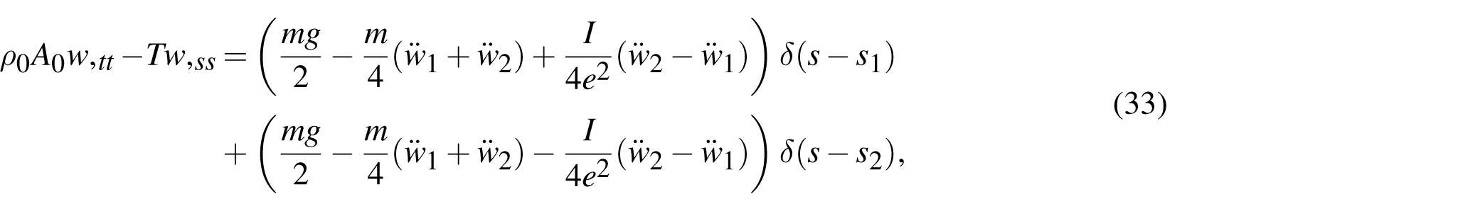
\begin{matrix} ẅ_{1} = ẅ (s_{1}, t) = ẅ_{m} - e {\overset{\cdot\cdot}{θ}}_{m} and ẅ_{2} = ẅ (s_{2}, t) = ẅ_{m} + e {\overset{\cdot\cdot}{θ}}_{m} . \end{matrix}

(13)

Using the kinematic relations in equation (13), and substituting the expressions for $ẅ_{m}$ and ${\overset{\cdot\cdot}{θ}}_{m}$ into equation (11), the equation of motion (EOM) of the system is expressed in terms of the inertial accelerations at the two point contacts of the moving mass as follows

\begin{matrix} \begin{matrix} ρ_{0} A_{0} w,_{tt} - [Tw,_{s}],_{s} & = (\frac{mg}{2} - \frac{m}{4} (ẅ_{1} + ẅ_{2}) + \frac{I}{4 e^{2}} (ẅ_{2} - ẅ_{1})) δ (s - s_{1}) \\ + (\frac{mg}{2} - \frac{m}{4} (ẅ_{1} + ẅ_{2}) - \frac{I}{4 e^{2}} (ẅ_{2} - ẅ_{1})) δ (s - s_{2}) . \end{matrix} \end{matrix}

(14)

It is worth noting that the EOM does not explicitly depend on $ẅ (s_{m}, t)$ . Consequently, an equivalent governing equation would be obtained if the formulation were expressed in terms of the actual center of mass position $r_{C} (t)$ . Furthermore, in equation (14), the inertial force associated with the contact point at $s_{1}$ acts at $s_{2}$ through Dirac delta functions, and vice versa.

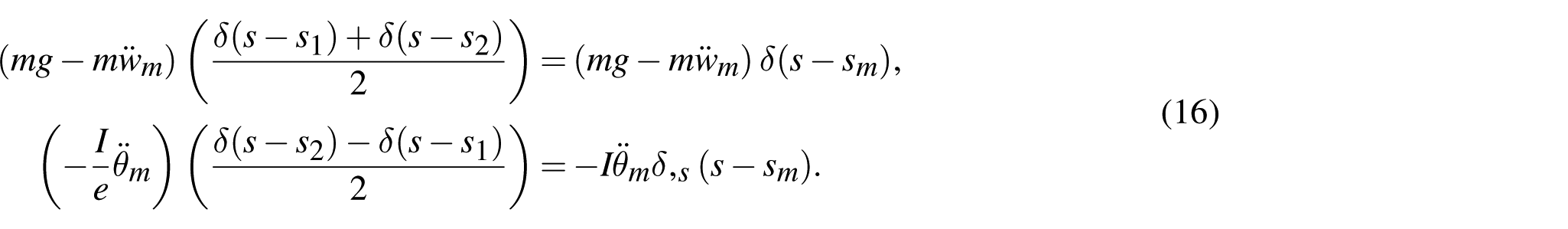
An alternative form of the governing equation (11) for a limiting case is derived by performing a Taylor expansion of the Dirac delta functions about $s_{m}$ in the limit $e \to 0$ , yielding

\begin{matrix} \begin{matrix} δ (s - s_{1}) = δ (s - s_{m} + e) & = δ (s - s_{m}) + eδ,_{s} (s - s_{m}) + O (e^{2}), \\ δ (s - s_{2}) = δ (s - s_{m} - e) & = δ (s - s_{m}) - eδ,_{s} (s - s_{m}) + O (e^{2}) . \end{matrix} \end{matrix}

(15)

From the right-hand side of equation (11) and using equation (15) and neglecting order $e^{2}$ , it follows that

\begin{matrix} \begin{matrix} (mg - m ẅ_{m}) (\frac{δ (s - s_{1}) + δ (s - s_{2})}{2}) & = (mg - m ẅ_{m}) δ (s - s_{m}), \\ (- \frac{I}{e} {\overset{\cdot\cdot}{θ}}_{m}) (\frac{δ (s - s_{2}) - δ (s - s_{1})}{2}) & = - I {\overset{\cdot\cdot}{θ}}_{m} δ,_{s} (s - s_{m}) . \end{matrix} \end{matrix}

(16)

As $e \to 0$ , equation (12) gives $θ_{m} = w,_{s} (s_{m}, t)$ , implying that the rotation of the mass is equal to the local slope of the string. Accordingly, upon applying equation (16), the governing equation (11) reduces to a representation involving Dirac delta (monopole) and dipole terms, expressed as

\begin{matrix} ρ_{0} A_{0} w,_{tt} - [Tw,_{s}],_{s} = [mg - mẅ (s_{m}, t)] δ (s - s_{m}) - Iẅ,_{s} (s_{m}, t) δ,_{s} (s - s_{m}) . \end{matrix}

(17)

This equation is identical to that employed in [9] and may also be derived using an energy-based formulation, as detailed in Appendix 1. It is important to note, however, that equation (17) represents the limiting case as $e \to 0$ , whereas equations (11) and (14) are valid for the regime $e ≪ L_{0}$ . In equation (17), the dipole term captures the effect of two closely spaced transverse forces acting at $s_{m}$ as $e \to 0$ , which formally introduces a point moment. While this representation is mathematically well-defined, it should be interpreted as a limiting case of force pairs rather than a true applied moment, since an ideal string (even under tension) does not possess bending rigidity and therefore cannot resist a moment in the same way as a beam. Accordingly, equation (14) provides the physically consistent description in terms of two separated transverse forces, while the moment term emerges only in the limiting sense.

3. Non-dimensional EOM

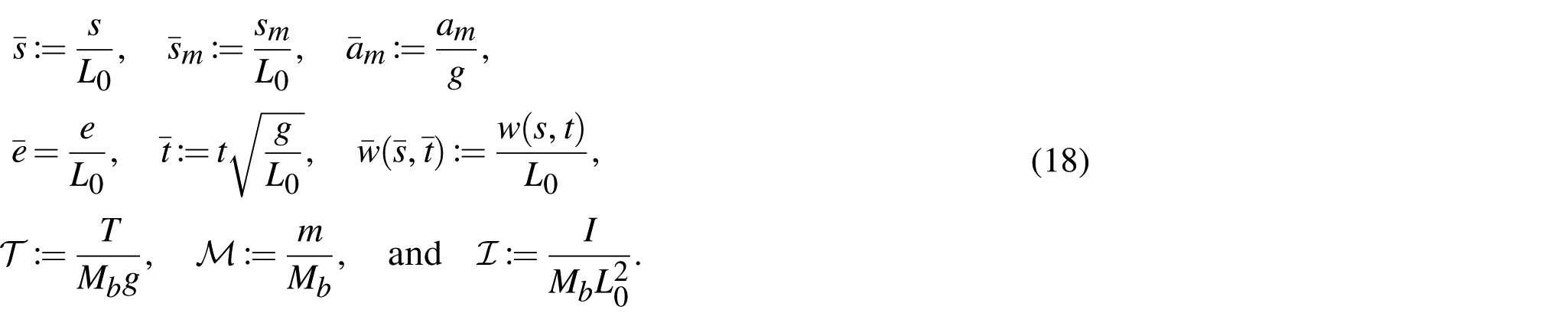
The following non-dimensional variables and parameters are introduced to get the non-dimensional form of the governing EOM

\begin{matrix} \begin{matrix} \bar{s} & : = \frac{s}{L_{0}}, {\bar{s}}_{m} : = \frac{s_{m}}{L_{0}}, ā_{m} : = \frac{a_{m}}{g}, \\ ē & = \frac{e}{L_{0}}, \bar{t} : = t \sqrt{\frac{g}{L_{0}}}, \bar{w} (\bar{s}, \bar{t}) : = \frac{w (s, t)}{L_{0}}, \\ T & : = \frac{T}{M_{b} g}, M : = \frac{m}{M_{b}}, and I : = \frac{I}{M_{b} L_{0}^{2}} . \end{matrix} \end{matrix}

(18)

Here, $M_{b} = ρ_{0} A_{0} L_{0}$ denotes the total mass of the string. The quantity $M$ denotes the ratio of the moving mass to the mass of the string. $T$ denotes the ratio of the string tension to its gravitational weight, while $I$ represents the ratio of the moment of inertia of the moving mass about point C to three times the moment of inertia of a rigid rod, dimensionally equivalent to the string, taken about one end. ē is the non-dimensional eccentric distance of the contact points from the center. For the sake of simplicity, overbars from all the variables are removed in the following texts.

Substituting non-dimensional variables from equation (18), into equation (14), we get

\begin{matrix} \begin{matrix} w,_{tt} - [T w,_{s}],_{s} & = (\frac{M}{2} - \frac{M}{4} (ẅ_{1} + ẅ_{2}) + \frac{μ^{2} M}{4} (ẅ_{2} - ẅ_{1})) δ (s - s_{1}) \\ + (\frac{M}{2} - \frac{M}{4} (ẅ_{1} + ẅ_{2}) - \frac{μ^{2} M}{4} (ẅ_{2} - ẅ_{1})) δ (s - s_{2}) \end{matrix} \end{matrix}

(19)

Collecting common variables, it simplifies to

\begin{matrix} \begin{matrix} w,_{tt} - [T w,_{s}],_{s} & = \frac{M}{4} (2 - (1 + μ^{2}) ẅ_{1} - (1 - μ^{2}) ẅ_{2}) δ (s - s_{1}) \\ + \frac{M}{4} (2 - (1 - μ^{2}) ẅ_{1} - (1 + μ^{2}) ẅ_{2}) δ (s - s_{2}) \end{matrix} \end{matrix}

(20)

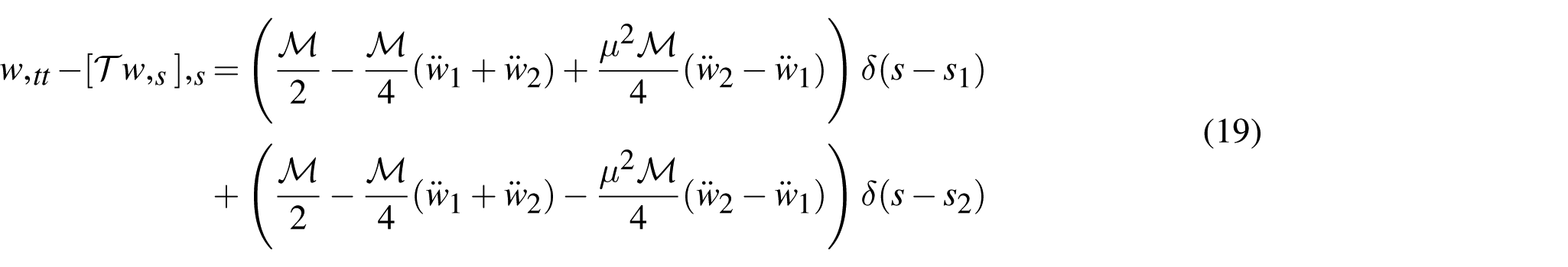
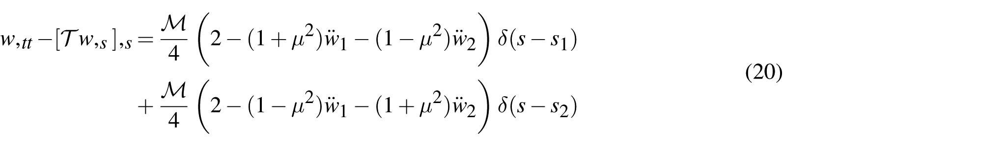
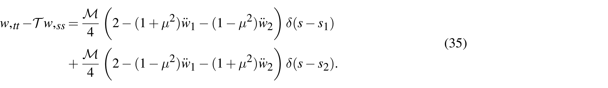
This equation represents the final non-dimensional EOM of a string interacting with a moving mass through two contact points located at the non-dimensional material coordinates $s_{1}$ and $s_{2}$ . The formulation involves five non-dimensional parameters: the tension–string weight ratio $T$ , the moving mass–string mass ratio $M$ , the gyration factor $μ$ , the half-distance between the two contact points $e$ , and the prescribed motion of the mass $s_{m}$ (or $v_{m}$ for uniformly moving mass). e and $s_{m}$ , which enter the equation through Dirac delta functions and the inertial acceleration $ẅ_{1}$ and $ẅ_{2}$ . For an accelerating prescribed motion $s_{m} = s_{m 0} + v_{m} t + 1 ∕ 2 a_{m} t^{2}$ introduces three parameters: the initial position $s_{m 0}$ along the undeformed string, the velocity $v_{m}$ , and the acceleration $a_{m}$ of the moving mass.

Equation (20) provides a general framework for analyzing linear dynamic problems under various boundary conditions. Before addressing specific cases and performing the parametric study presented in the following section, the continuous EOM is discretized using the Galerkin method.

4. Discretized governing equation

To discretize the non-dimensional EOM (20), we have employed the Galerkin method (GM) [2]. Let $W_{j} (s)$ be the trial functions that satisfy the essential boundary condition. Therefore, the non-dimensional transverse displacement can be written as follows

\begin{matrix} w (s, t) = \sum_{j = 1}^{N} W_{j} (s) p_{j} (t) . \end{matrix}

(21)

Here, $p_{j} (t)$ is the abstract modal coordinate of the jth trial function and N is the number of terms considered in the truncated solution series. In addition, the trial functions must satisfy the orthogonality property

\begin{matrix} \int_{0}^{1} W_{i} (s) W_{j} (s) ds = δ_{ij}, \end{matrix}

(22)

where $δ_{ij}$ is the Kronecker delta operator.

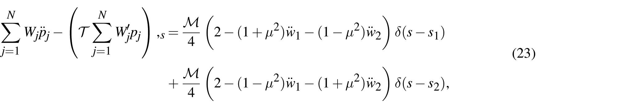
Substituting the assumed solution given by equation (21) into equation (20) and expanding all terms, we get

\begin{matrix} \begin{matrix} \sum_{j = 1}^{N} W_{j} {\overset{\cdot\cdot}{p}}_{j} - (T \sum_{j = 1}^{N} W_{j}^{'} p_{j}),_{s} & = \frac{M}{4} (2 - (1 + μ^{2}) ẅ_{1} - (1 - μ^{2}) ẅ_{2}) δ (s - s_{1}) \\ + \frac{M}{4} (2 - (1 - μ^{2}) ẅ_{1} - (1 + μ^{2}) ẅ_{2}) δ (s - s_{2}), \end{matrix} \end{matrix}

(23)

where $ẅ_{1}$ and $ẅ_{2}$ can be written using equations (21), (5), and (7), as follows

\begin{matrix} \begin{matrix} ẅ_{1} & = \sum_{j = 1}^{N} ({\overset{\cdot\cdot}{s}}_{m} W_{j}^{'} p_{j} + ṡ_{m}^{2} W_{j}^{″} p_{j} + 2 ṡ_{m} W_{j}^{'} ṗ_{j} + W_{j} {\overset{\cdot\cdot}{p}}_{j}) |_{s = (s_{m} - e)}, \\ ẅ_{2} & = \sum_{j = 1}^{N} ({\overset{\cdot\cdot}{s}}_{m} W_{j}^{'} p_{j} + ṡ_{m}^{2} W_{j}^{″} p_{j} + 2 ṡ_{m} W_{j}^{'} ṗ_{j} + W_{j} {\overset{\cdot\cdot}{p}}_{j}) |_{s = (s_{m} + e)} . \end{matrix} \end{matrix}

(24)

For a uniformly moving mass, ${\overset{\cdot\cdot}{s}}_{m} = 0$ . The remaining terms depend on the state variables $p_{j} (t)$ , $ṗ_{j} (t)$ , and ${\overset{\cdot\cdot}{p}}_{j} (t)$ , with $j = 1, \dots, N$ , and therefore contribute to the mass, damping, and stiffness matrices in the discretized EOM.

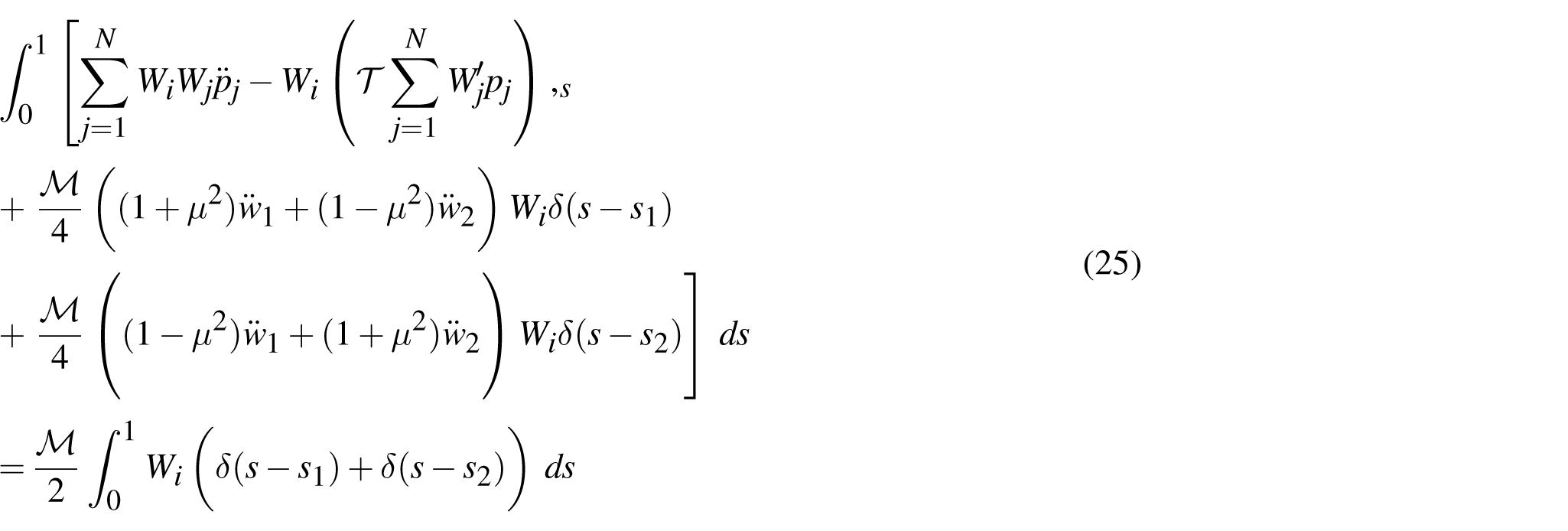
Now, let us take the inner product of the above equation with $W_{i} (s)$ over the non-dimensional domain length of the string, i.e. from 0 to 1, to get the ith EOM as follows

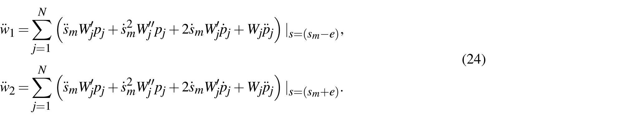
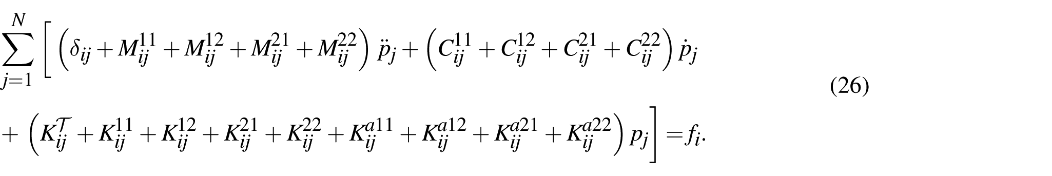
\begin{matrix} \begin{matrix} \int_{0}^{1} [\sum_{j = 1}^{N} W_{i} W_{j} {\overset{\cdot\cdot}{p}}_{j} - W_{i} (T \sum_{j = 1}^{N} W_{j}^{'} p_{j}),_{s} \\ + \frac{M}{4} ((1 + μ^{2}) ẅ_{1} + (1 - μ^{2}) ẅ_{2}) W_{i} δ (s - s_{1}) \\ + \frac{M}{4} ((1 - μ^{2}) ẅ_{1} + (1 + μ^{2}) ẅ_{2}) W_{i} δ (s - s_{2})] ds \\ = \frac{M}{2} \int_{0}^{1} W_{i} (δ (s - s_{1}) + δ (s - s_{2})) ds \end{matrix} \end{matrix}

(25)

From equation (24), it follows that the inertial acceleration terms $ẅ_{1}$ and $ẅ_{2}$ are evaluated at $s = s_{m} (t) \pm e$ . Consequently, these terms depend only on time $t$ and can therefore be taken outside the integration with respect to $s$ . The remaining terms are simplified by invoking the orthogonality condition given in equation (22) and the properties of the Dirac delta function [43]. Hence, the ith EOM can be concisely written as

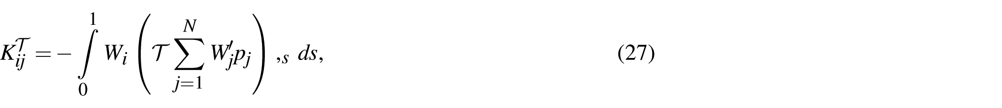
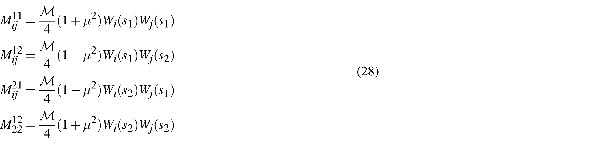
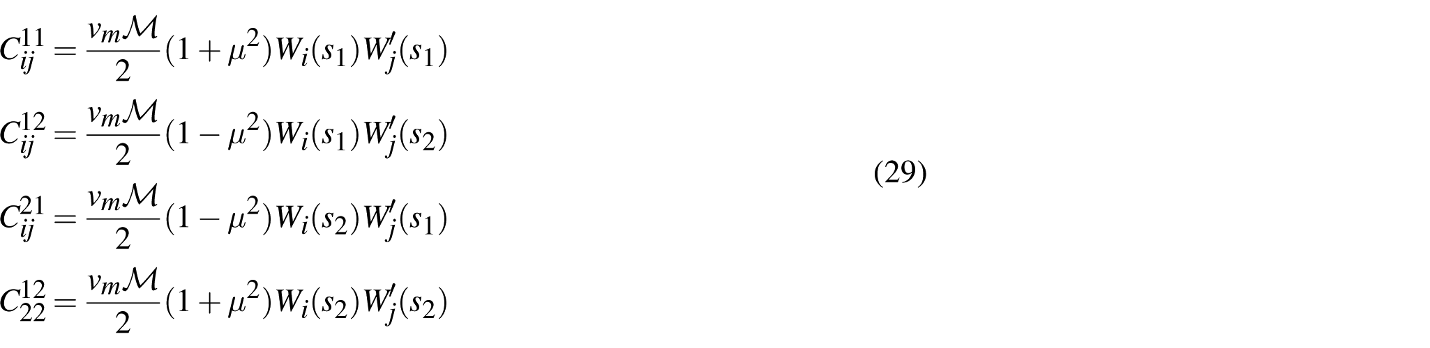
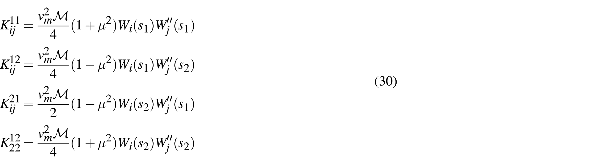
\begin{matrix} \begin{matrix} \sum_{j = 1}^{N} [(δ_{ij} + M_{ij}^{11} + M_{ij}^{12} + M_{ij}^{21} + M_{ij}^{22}) {\overset{\cdot\cdot}{p}}_{j} + (C_{ij}^{11} + C_{ij}^{12} + C_{ij}^{21} + C_{ij}^{22}) ṗ_{j} \\ + (K_{ij}^{T} + K_{ij}^{11} + K_{ij}^{12} + K_{ij}^{21} + K_{ij}^{22} + K_{ij}^{a 11} + K_{ij}^{a 12} + K_{ij}^{a 21} + K_{ij}^{a 22}) p_{j}] = f_{i} . \end{matrix} \end{matrix}

(26)

for $i = 1, 2, 3, \dots, N$ gives the discrete form N equations. $δ_{ij}$ is the Kronecker delta operator, and the remaining terms can be defined as follows

\begin{matrix} K_{ij}^{T} = - \int_{0}^{1} W_{i} (T \sum_{j = 1}^{N} W_{j}^{'} p_{j}),_{s} ds, \end{matrix}

(27)

\begin{matrix} \begin{matrix} M_{ij}^{11} & = \frac{M}{4} (1 + μ^{2}) W_{i} (s_{1}) W_{j} (s_{1}) \\ M_{ij}^{12} & = \frac{M}{4} (1 - μ^{2}) W_{i} (s_{1}) W_{j} (s_{2}) \\ M_{ij}^{21} & = \frac{M}{4} (1 - μ^{2}) W_{i} (s_{2}) W_{j} (s_{1}) \\ M_{22}^{12} & = \frac{M}{4} (1 + μ^{2}) W_{i} (s_{2}) W_{j} (s_{2}) \end{matrix} \end{matrix}

(28)

\begin{matrix} \begin{matrix} C_{ij}^{11} & = \frac{v_{m} M}{2} (1 + μ^{2}) W_{i} (s_{1}) W_{j}^{'} (s_{1}) \\ C_{ij}^{12} & = \frac{v_{m} M}{2} (1 - μ^{2}) W_{i} (s_{1}) W_{j}^{'} (s_{2}) \\ C_{ij}^{21} & = \frac{v_{m} M}{2} (1 - μ^{2}) W_{i} (s_{2}) W_{j}^{'} (s_{1}) \\ C_{22}^{12} & = \frac{v_{m} M}{2} (1 + μ^{2}) W_{i} (s_{2}) W_{j}^{'} (s_{2}) \end{matrix} \end{matrix}

(29)

\begin{matrix} \begin{matrix} K_{ij}^{11} & = \frac{v_{m}^{2} M}{4} (1 + μ^{2}) W_{i} (s_{1}) W_{j}^{″} (s_{1}) \\ K_{ij}^{12} & = \frac{v_{m}^{2} M}{4} (1 - μ^{2}) W_{i} (s_{1}) W_{j}^{″} (s_{2}) \\ K_{ij}^{21} & = \frac{v_{m}^{2} M}{2} (1 - μ^{2}) W_{i} (s_{2}) W_{j}^{″} (s_{1}) \\ K_{22}^{12} & = \frac{v_{m}^{2} M}{4} (1 + μ^{2}) W_{i} (s_{2}) W_{j}^{″} (s_{2}) \end{matrix} \end{matrix}

(30)

\begin{matrix} \begin{matrix} K_{ij}^{a 11} & = \frac{a_{m} M}{4} (1 + μ^{2}) W_{i} (s_{1}) W_{j}^{'} (s_{1}) \\ K_{ij}^{a 12} & = \frac{a_{m} M}{4} (1 - μ^{2}) W_{i} (s_{1}) W_{j}^{'} (s_{2}) \\ K_{ij}^{a 21} & = \frac{a_{m} M}{2} (1 - μ^{2}) W_{i} (s_{2}) W_{j}^{'} (s_{1}) \\ K_{22}^{a 12} & = \frac{a_{m} M}{4} (1 + μ^{2}) W_{i} (s_{2}) W_{j}^{'} (s_{2}) \end{matrix} \end{matrix}

(31)

\begin{matrix} f_{i} = \frac{M}{2} (W_{i} (s_{1}) + W_{i} (s_{2})) . \end{matrix}

(32)

For a given linearized string system carrying a moving mass and subject to appropriate boundary conditions, equation (26) can be integrated to obtain the system response. In the following section, two linearized string systems with a moving mass are examined: (1) a stretched string subjected to a uniformly moving mass, considered to investigate the trajectory paradox reported in earlier studies [5,6,29] when the moving body is modeled as a point mass; and (2) a vertically hanging string carrying a moving mass, which, to the best of our knowledge, has not been previously addressed in the literature.

5. Stretched string subjected to uniformly moving mass

Consider a stretched string carrying a moving mass, as illustrated in Figure 2. In a fixed RHOCF ${\tilde{G}, O, {\hat{g}}_{j}}$ , the string is fixed at two boundaries, O and $B_{△}$ , and is lying horizontally along the line $O B_{△}$ . Gravity acts perpendicular to this reference configuration, in the direction ${\hat{g}}_{2}$ .

Figure 2.

A horizontal linearized stretched string subjected to a moving mass. The mass possesses finite rotary inertia and touches the string a two close points.

The string is assumed to be under a constant and uniform tension T, which remains unchanged during the motion of the mass. The tension is sufficiently large that any initial sag of the string due to gravity is neglected. Nevertheless, gravitational forces act on the moving mass in the transverse direction and therefore influence the system dynamics. This modeling framework is standard in studies of stretched strings subjected to moving point masses [5,6,29].

In contrast to classical formulations that represent the moving body as a single point mass, the present work extends the model by introducing two closely spaced point contacts. This refinement enables the inclusion of the rotary motion of the moving mass, as formulated in Section 2.

All remaining characteristic parameters of the system are retained as defined in Section 2. With the length of $O B_{△}$ set to $L_{0}$ and the string has a constant and uniform tension T, the governing equation (14) reduces to

\begin{matrix} \begin{matrix} ρ_{0} A_{0} w,_{tt} - Tw,_{ss} & = (\frac{mg}{2} - \frac{m}{4} (ẅ_{1} + ẅ_{2}) + \frac{I}{4 e^{2}} (ẅ_{2} - ẅ_{1})) δ (s - s_{1}) \\ + (\frac{mg}{2} - \frac{m}{4} (ẅ_{1} + ẅ_{2}) - \frac{I}{4 e^{2}} (ẅ_{2} - ẅ_{1})) δ (s - s_{2}), \end{matrix} \end{matrix}

(33)

with the boundary conditions at both taut ends as follows

\begin{matrix} w (0, t) = 0, and w (L_{0}, t) = 0 . \end{matrix}

(34)

Using the non-dimensional parameters defined in (18), and subsequently dropping the overbars for convenience, the simplified non-dimensional form of the EOM is given by

\begin{matrix} \begin{matrix} w,_{tt} - T w,_{ss} & = \frac{M}{4} (2 - (1 + μ^{2}) ẅ_{1} - (1 - μ^{2}) ẅ_{2}) δ (s - s_{1}) \\ + \frac{M}{4} (2 - (1 - μ^{2}) ẅ_{1} - (1 + μ^{2}) ẅ_{2}) δ (s - s_{2}) . \end{matrix} \end{matrix}

(35)

The non-dimensional boundary conditions at the two ends reduce to

\begin{matrix} w (0, t) = 0, and w (1, t) = 0 . \end{matrix}

(36)

These boundary conditions are satisfied by the following trial functions, which are employed in the truncated Galerkin solution given in equation (21). In addition, the chosen trial functions satisfy the required orthogonality properties (22).

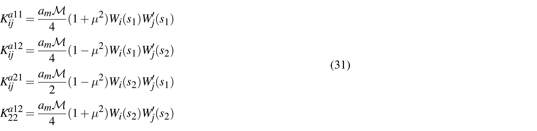
\begin{matrix} W_{j} (s) = \sqrt{2} \sin (ω_{j} s), for ω_{j} = jπ . \end{matrix}

(37)

Substituting these trial functions into equation (25) results in the discretized EOM (26). The associated components of mass, damping, and stiffness matrices and force vector are defined by equations (28)–(32), respectively. For uniformly prescribed motion of the mass, the relative (prescribed) acceleration vanishes, i.e. ${\overset{\cdot\cdot}{s}}_{m} = a_{m} = 0$ , and consequently the stiffness contributions associated with this acceleration, given by equation (31), do not contribute to the system dynamics. In addition, the stiffness term defined in equation (27) admits a particularly simplified form, as below

\begin{matrix} K_{ij}^{T} = T ω_{j}^{2} δ_{ij} . \end{matrix}

(38)

The simplified discretized EOM (26) are integrated numerically using a fourth-order Runge–Kutta scheme implemented in MATLAB software.

5.1. Results and discussions

The discretized EOM (26) depends on five parameters, namely, $T$ , $M$ , μ, e, and $v_{m}$ , for uniformly moving mass. To validate the present formulation, results for uniformly moving cases are first compared with existing studies on moving point forces [2,44] and moving point masses [6]. This is achieved by setting $μ = 0$ and $e = 0$ .

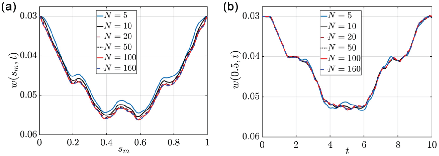
Figure 3 illustrates the convergence of the Galerkin solution, obtained from equation (21) using the trial functions in equation (37), for a uniformly moving point mass on a stretched string. Parameters values are taken as $T = 1$ , $M = 0.2$ , $μ = 0$ , $e = 0$ , and $v_{m} = 0.1 c$ . Here, $c = \sqrt{T}$ is the dimensionless transverse wave speed in the stretched string. Figure 3(a) and (b) presents, respectively, the mass trajectory and the time-history response of the string midpoint for increasing values of $N$ . The midpoint response is observed to converge more rapidly than the trajectory. As $N$ increases, both responses approach a stable solution, with the curves for $N = 100$ and $N = 160$ essentially overlapping. Based on this convergence behavior, $N = 150$ is adopted for all subsequent plots and parametric studies unless it is specified.

Figure 3.

Convergence of (a) the trajectory of the moving point mass and (b) midpoint response of the string for $T = 1$ , $M = 0.2$ , $μ = 0$ , $e = 0$ , and $v_{m} = 0.1 c$ .

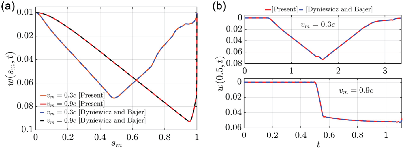
Figure 4(a) and (b) compares the responses obtained using the present Galerkin-based formulation (equation (21)) with those reported by Dyniewicz and Bajer [6], who employed the Fourier sine integral transformation. The characteristic parameters used in [6] are non-dimensionalized according to equation (18). Upon simplification, it is observed that, for the same number of modes $N$ , the discretized equations derived from both approaches are identical. Consequently, as shown in Figure 4, the mass trajectories and the midpoint time histories of the string coincide for both methods at velocities $v_{m} = 0.3 c$ and $v_{m} = 0.9 c$ . In Figure 4(a), the jump in the trajectory near $s_{m} = 1$ (the terminating boundary, $B_{△}$ ) for $v_{m} = 0.9 c$ is clearly visible. This behavior is consistent with the well-known trajectory paradox associated with a massless string model as reported in [5] and also discussed in Section 1.

Figure 4.

Comparison of (a) the trajectory of the moving point mass and (b) the midpoint response of the string for two velocities, $v_{m} = 0.3 c$ and $v_{m} = 0.9 c$ . Results obtained using the present Galerkin-based formulation are compared with those reported by Dyniewicz and Bajer [6], who employed the Fourier sine integral transformation. The parameter values are $T = 1$ , $M = 0.2$ , $μ = 0$ , $e = 0$ , and $N = 150$ taken for both methods.

Similarly, by setting $M = 0$ , in all terms of equation (26) except the force term $f_{i}$ , defined in equation (32), thereby reducing the formulation to that of a stretched string subjected to a moving point force. The force magnitude is $Q = mg$ , which follows from neglecting the inertial contribution in equation (8); for a point force ( $e = 0$ ), this yields $Q = Q_{s_{1}} + Q_{s_{2}} = mg$ . The response of such systems is well documented in the literature [2,44]. Furthermore, neglecting axial displacements under the quasi-static stretch assumption adopted in [2], the governing equations match exactly with those of the present moving point-force model. Figure 5 illustrates the trajectories and midpoint responses for two values of $M = 0.1$ and $M = 1$ . The force is moving at a uniform speed of $v_{m} = 0.1 c$ . An increase in the force magnitude leads to larger transverse displacements of the string, a trend that is also observed in the moving point-mass case.

Figure 5.

(a) The trajectory of the moving point force and (b) the midpoint response of the string for two values of mass ratio, $M = 0.2$ and $M = 1$ . Results obtained for parameter values are $T = 1$ , $v_{m} = 0.1 c$ , $μ = 0$ , and $e = 0$ .

Thus far, the formulation has been validated by reducing it to the limiting cases of a moving point mass and, further, a moving point force. The primary objective of the two-point contact formulation, however, is to investigate the influence of rotary inertia on the trajectory paradox for an inertial (massive) string. This is achieved by assigning non-zero values to the parameters μ and e for a uniformly moving mass. In essence, a parametric study is conducted to examine how the trajectory paradox evolves as the idealized moving point mass is replaced by a more physically realistic body (cable-climbing robot with dual-point contact) that possesses finite rotary inertia.

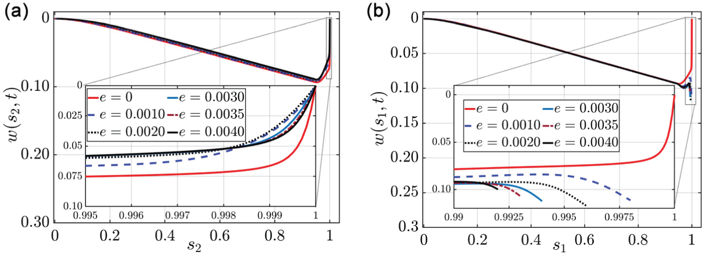
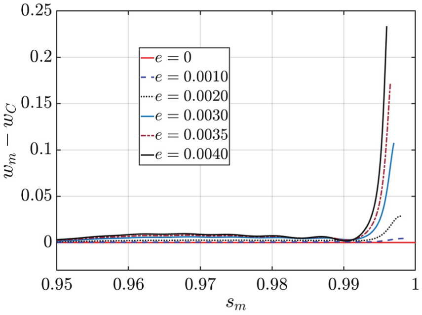
For $T = 1$ , $M = 0.2$ , $v_{m} = 0.9 c$ , $μ = 1$ , and $N = 150$ , Figure 6 shows the trajectories at the two contact points ( $s_{1}$ and $s_{2}$ ) of the moving mass for small eccentricities ( $e ≪ 1$ ). The case $μ = 1$ represents two identical point masses of magnitude $m ∕ 2$ located at $s_{1}$ and $s_{2}$ , separated by a distance $2 e$ and moving with the same velocity. From equation (35), the forces at the two contact points act independently for $μ = 1$ , such that $Q_{s_{1}}$ does not influence the forcing at $s_{2}$ , and vice versa. For $e \neq 0$ , motion begins with the rear contact at the origin and ends when the front contact reaches $s = 1$ , giving a total travel distance of $1 - 2 e$ .

Figure 6.

Trajectories of (a) the front and (b) rear contact points of the moving mass for varying values of e. Insets show magnified views near the end of motion, at $s = 1$ for the front contact and $s = 1 - 2 e$ for the rear contact.

For $e = 0$ , the trajectories in Figure 6(a) and (b) coincide, consistent with the behavior of an equivalent single moving point mass. As e increases, the trajectories shift away from the boundary at $s = 1$ and become less steep, as illustrated in the insets. Near the terminating boundary, the paths of the front and rear contacts diverge from each other for the same value of e. The front contact reaches $s_{2} = 1$ in a manner similar to a moving point mass. As noted in [6], such a mass on an inertial string exhibits a displacement jump near the boundary, analogous to the trajectory paradox reported in [5] for a massless string. The same jump is observed here at the front contact, as shown in the inset of Figure 6(a).

In contrast, the rear contact’s motion ends at $s = 1 - 2 e$ . When rotary inertia is present ( $e \neq 0$ ), its trajectory evolves in the opposite direction to that of the front end near the boundary, as illustrated in the inset of Figure 6(b). These observations indicate that, although the two-contact mass predominantly moves horizontally along the linearized string, away from the terminating boundary, the trajectory paradox near the boundary produces opposing stretching at the two contact points, leading to a temporary, almost vertical reorientation of the mass.

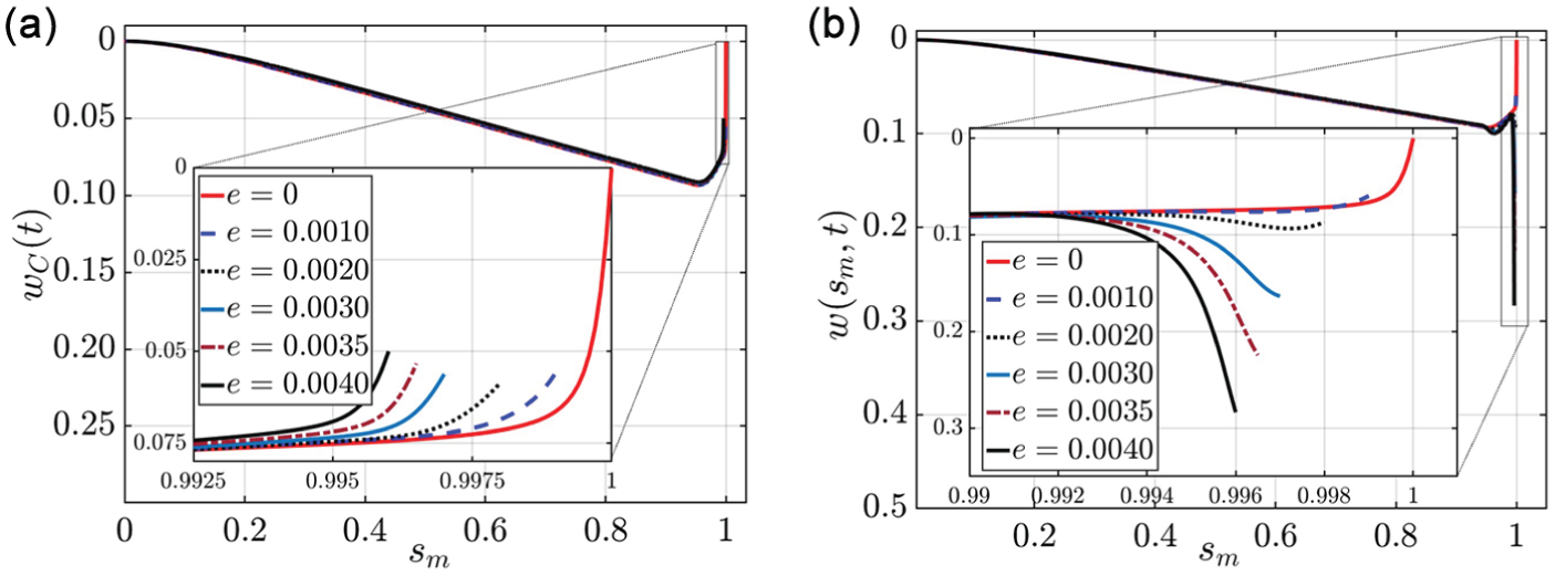
For the same set of parameters, Figure 7(a) and (b) shows the actual trajectory $r_{C} (t)$ and the trajectory $r_{m} (t)$ of the string material point at $s = s_{m} (t)$ , respectively. The latter can be interpreted as the virtual center of the moving mass, as defined in equation (3). Away from the terminating boundary, both trajectories coincide and follow the same path. However, near the boundary, when the front contact $s_{2} \to 1$ , and the centers $s_{m} \to 1 - e$ , the insets reveal a clear deviation. Increasing the eccentricity parameter e leads to steeper trajectories near $s = 1 - e$ . While the actual and virtual centers coincide away from the boundary $B_{△}$ , consistent with the linear dynamics of the string, they diverge as the mass approaches $B_{△}$ due to the jump as $s_{2} \to 1$ .

Figure 7.

Variation of the actual and virtual trajectories of the moving mass for different values of e. The insets present an enlarged view near the termination of the motion.

Based on these results, Figure 8 illustrates, for same parameters, the separation between the actual and virtual centers of the moving mass for different values of $e$ . This separation arises solely from the difference between the transverse displacement of the mass center and that of the corresponding string material point at $s_{m}$ . Since both the actual and virtual points share the same axial location $s_{m}$ , the separation is simply $w_{m} - w_{C}$ . As shown in Figure 8, increasing $e$ leads to a drastic growth in separation, as $s_{m} \to 1 - e$ . When $e = 0$ , corresponding to a moving point mass, the separation vanishes.

Figure 8.

Separation between the actual and virtual center of the moving mass for different values of e near $s_{m} = 1 - e$ .

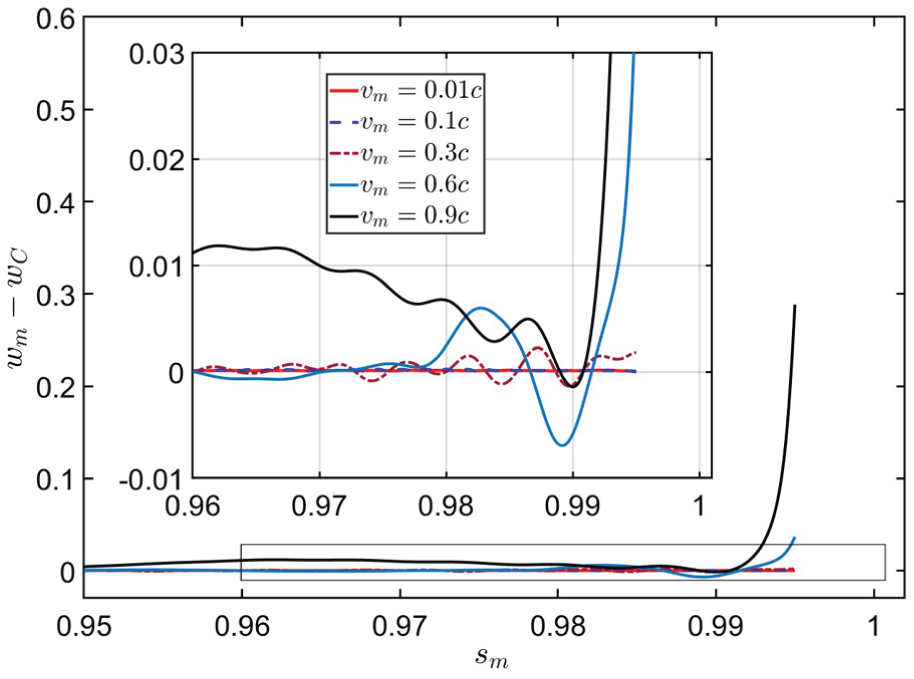
For $T = 1$ , $M = 0.2$ , $μ = 1$ , $e = 0.005$ , and $N = 150$ , Figure 9 shows the separation between the actual and virtual centers near $s_{m} = 1 - e$ for different prescribed velocities $v_{m}$ of the moving mass. At low velocity ( $v_{m} = 0.01 c$ ), the separation is negligible. As $v_{m}$ increases, a distinct divergence appears near the boundary, as illustrated in the enlarged inset of Figure 9. This behavior indicates the emergence of a trajectory jump at higher velocities. At lower velocities, the jump remains minimal [6], resulting in an insignificant separation between the two trajectories.

Figure 9.

Separation between the actual and virtual center of the moving mass for different velocity $v_{m}$ of the mass near $s_{m} = 1 - e$ .

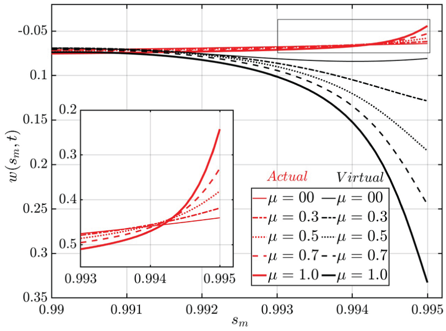
In the above plots, $μ = 1$ is considered. The separation and trajectory behavior shown in Figures 6 –9 remains consistent for all values of $μ$ , as illustrated in Figure 10. This figure presents the actual and virtual trajectories near $s_{m} = 1 - e$ . The results are obtained for $T = 1$ , $M = 0.2$ , $v_{m} = 0.9 c$ , and $e = 0.005$ . It is observed that increasing $μ$ leads to behavior similar to that previously observed for increasing $e$ . This is expected because, as defined in equation (2), the moment of inertia is given by $I = m {(μe)}^{2}$ ; hence, increasing either $e$ and $μ$ effectively enhances the rotary inertia of the moving mass. This figure clearly shows the bifurcation of the actual and the virtual center of the moving mass for different values of μ initiated after $s_{m} = 0.99$ .

Figure 10.

The actual and virtual trajectories of the moving mass for different values of μ as $s_{m} \to 1 - e$ .

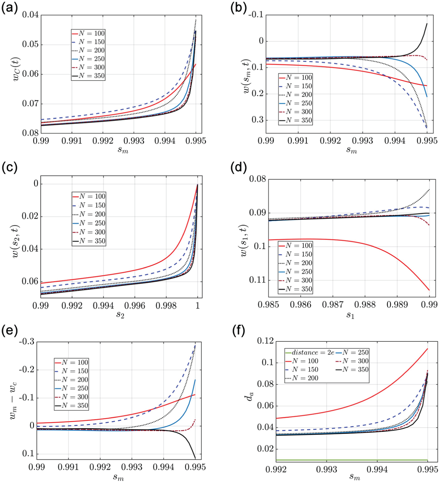
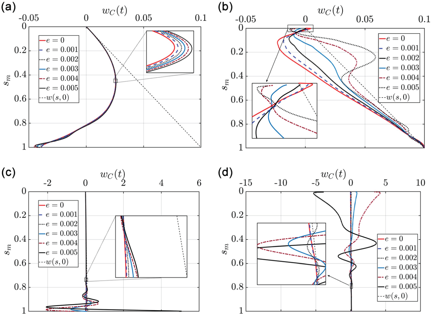
The large separation between the actual and virtual centers of mass near the terminating boundary $B_{△}$ indicates a failure of the linearized string model and a consequent breakdown of its underlying assumptions. In particular, the condition $w_{C} \approx w_{m}$ is expected for a linearized model of a string, but it is no longer satisfied when the jump occurs in a narrow region near $B_{△}$ for the trajectory at $s_{2}$ . Although the trajectory exhibits convergence on the scale of the string length similar to the behavior shown in Figure 3, even for the two-point contact moving mass, significant deviations emerge near the boundary. To examine this behavior in detail, a comprehensive convergence study is therefore performed near the terminating boundary, as presented in Figure 11. The parameters used in this analysis are $T = 1$ , $M = 0.2$ , $v_{m} = 0.9 c$ , $μ = 1$ , and $e = 0.005$ .

Figure 11.

Convergence behavior near the terminating boundary $B_{△}$ with increasing numbers of terms in the truncated Galerkin solution. (a) The actual trajectories, (b) the virtual trajectories, (c) the transverse displacement of the front contact, (d) the transverse displacement of the rear contact, (e) the separation between the actual and virtual trajectories, and (f) the actual separation between the two contacts; the green line indicates the assigned distance $2 e$ .

Figure 11 presents the evolution of selected variables obtained from the truncated Galerkin solution (equation (21)) as the number of modes N increases. The analysis focuses on a narrow region, namely, $s_{m} \in [0.99, 0.995]$ , $s_{2} \in [0.99, 1]$ , and $s_{1} \in [0.985, 0.99]$ , corresponding to the stage where the front contact of the mass approaches the terminating boundary $B_{△}$ . In this regime, the trajectory paradox, manifested as a jump, becomes evident. Figure 11(a) and (b) presents the actual and virtual trajectories of the center of mass, respectively. The trajectories of the string’s material points in contact with the moving mass are shown in Figure 11(c) and (d), corresponding to the front contact point at $s_{2}$ and the rear contact point at $s_{1}$ . Figure 11(e) shows the separation between the actual and virtual centers of mass for different values of N. Figure 11(f) depicts the actual distance between the two contact points of the moving mass on the string, defined as $d_{a} = \sqrt{{(w_{2} - w_{1})}^{2} + {(2 e)}^{2}}$ , where $w_{1}$ and $w_{2}$ are defined in equation (12). For small transverse displacements, ${(w_{2} - w_{1})}^{2}$ is negligible, and the actual contact distance closely matches the assigned separation $2 e$ , indicated by the green line in Figure 11(f). However, due to the jump near the boundary, a larger difference arises between the actual and assigned contact separation.

As $N$ increases, all trajectories and separation measures exhibit slow convergence, a characteristic of the trajectory paradox. Similar behavior was reported by Dyniewicz et al. [6], who showed that for a moving point mass on an inertial string, the trajectory converges toward $s_{m} = 1$ , as higher values of $N$ cause the mass to approach a jump slowly. Using the same formulation, analysis of the slope profiles at the moving mass reveals a sharp increase as $s_{m} \to 1$ , indicating divergence of the slope near the boundary. This rapid growth occurs as the rotation angle approaches $9 0^{\circ}$ , driven by the pronounced curvature of the trajectory in the vicinity of the boundary.

Comparable findings were reported by Ferretti et al. [29], who incorporated axial deformation in a massive string model. They observed convergence near $s_{m} = 1$ and found that increasing the Galerkin discretization order results in larger axial displacements of the moving mass. In agreement with these findings, the present two-point contact model exhibits an increasing slope, with the trajectory jump becoming sharper as $s_{2} \to 1$ for higher values of N (see Figure 11(c)). This qualitative trend holds across the entire range of μ values considered for $e = 0.005$ , indicating the robustness of the observed behavior.

A closer examination of Figure 11 indicates that increasing N delays the separation between successive curves corresponding to higher discretization orders. This trend suggests that, for sufficiently large N, the jump at the front contact initiates closer to $s_{2} = 1$ (see Figure 11(c)). A similar behavior is observed in the actual trajectory (Figure 11(a)), where the jump occurs progressively nearer to $s_{m} = 1 - e$ as N increases. The virtual trajectories (Figure 11(b)) exhibit a change in displacement sign with increasing N and tend toward a finite nonzero value for sufficiently large N. Consistent trends are also evident in the rear contact displacement at $s_{1}$ (Figure 11(d)) and in the separation between the actual and virtual centers (Figure 11(e)). Furthermore, the distance between the two contact points decreases with increasing N and approaches a finite limit, as shown in Figure 11(f).

In summary, this numerical example was used to conduct a parametric study aimed at investigating the trajectory paradox previously reported for a uniformly moving point mass, here extended to a more realistic moving-mass model with two-point contact with the string. Although the rotational inertia satisfies $I = m {(μe)}^{2}$ with $e ≪ 1$ in the non-dimensional formulation, significant deviations in the system response are observed near the terminating boundary $B_{△}$ . The results demonstrate that, even for this modified model, the trajectory paradox persists at $B_{△}$ , with variations in the nature of the associated jumps.

Now, a new system consisting of a hanging string carrying a moving mass is examined using the same formulation, with appropriate modifications. In this configuration, asymmetric boundary conditions arise due to the fixed upper end and the free lower end of the string, resulting in both ascending and descending motion of the mass. In the present study, the investigation is restricted to the case of a uniformly moving mass, although the formulation is developed for more general motion scenarios.

6. Hanging string carrying a moving mass

Figure 12 shows a planar hanging string carrying a moving mass. The string is fixed at the origin of the RHOCF ${\tilde{G}, O, {\hat{g}}_{j}}$ . Another end of the string ( $B_{t}$ ) is free. The acceleration due to gravity g is acting on the hanging string-moving mass system along ${\hat{g}}_{1}$ , not in the transverse direction as present in the case of a stretched string. The equilibrium configuration of the string is straight along ${\hat{g}}_{1}$ . The static and dynamic axial deformations in the string are ignored. The moving mass may move either downward (descends) from the fixed end O toward the free end $B_{t}$ , or upward (ascends) from $B_{t}$ toward the fixed end O.

Figure 12.

(a) Schematic of a linearized hanging string carrying a moving mass. Gravity g acts in the direction ${\hat{g}}_{1}$ . The dotted black line indicates the string’s initial displaced configuration, forming an angle $θ_{0}$ with the equilibrium position. (b) FBDs of the moving mass and the adjacent string element with which it interacts.

The string tension varies both spatially and temporally due to the action of gravity along the axial direction ${\hat{g}}_{1}$ and the time-dependent position of the moving mass. Based on the FBD shown in Figure 12(b), the LMB in equation (8) is accordingly modified as follows

\begin{matrix} mg {\hat{g}}_{1} - Q = m {\overset{\cdot\cdot}{r}}_{m} . \end{matrix}

(39)

In component form, the expressions in this equation are decomposed along ${\hat{g}}_{1}$ and ${\hat{g}}_{2}$ directions as follows

\begin{matrix} \begin{matrix} Q_{1} & = mg - m a_{m}, \end{matrix} \end{matrix}

(40)

\begin{matrix} Q_{2} = Q_{s_{1}} + Q_{s_{2}} = mẅ (s_{m}, t) . \end{matrix}

(41)

The net reaction force between the string and the moving mass is denoted by $Q = Q_{1} {\hat{g}}_{1} + Q_{2} {\hat{g}}_{2}$ . In the transverse direction ${\hat{g}}_{2}$ , the resultant reaction arises from forces acting at two discrete contact points along the string; accordingly, $Q_{2} = Q s_{1} + Q s_{2}$ , where the forces act at the material points $s_{1} (t)$ and $s_{2} (t)$ , as defined in equation (7). The AMB remains unchanged and is given by equation (9).

Since gravity does not explicitly influence the transverse motion of the moving mass, equation (41) and (9) imply that the reaction forces in equation (10) reduce to the following form as

\begin{matrix} Q_{s_{1}} = \frac{m}{2} ẅ_{m} - \frac{I}{2 e} {\overset{\cdot\cdot}{θ}}_{m} and Q_{s_{2}} = \frac{m}{2} ẅ_{m} + \frac{I}{2 e} {\overset{\cdot\cdot}{θ}}_{m} . \end{matrix}

(42)

It should be noted, however, that gravity influences the system implicitly through the string tension, which in turn affects $ẅ_{m}$ and ${\overset{\cdot\cdot}{θ}}_{m}$ as they appear in the above equations.

The axial reaction component $Q_{1}$ acts on the string at the location of the moving mass, i.e. at $s = s_{m}$ , along the ${\hat{g}}_{1}$ direction, as shown in Figure 12(b), together with the weight of the string below that cross-section. For small transverse displacements and for small eccentric distance e of the point contacts from the center of the moving mass, the string tension, which varies in space and time due to self-weight and the axial reaction force, can be expressed as follows

\begin{matrix} T (s, t) = {\begin{matrix} ρ_{0} A_{0} g (L_{0} - s) + mg - m a_{m}, & 0 \leq s \leq s_{m} \\ ρ_{0} A_{0} g (L_{0} - s), & s_{m} < s \leq L_{0} . \end{matrix} \end{matrix}

(43)

Note that the tension at the free end is zero. The portion of the string above the instantaneous axial position of the moving mass carries an additional uniform tension equal to $Q_{1}$ at that time. However, due to the inertial contribution within $Q_{1}$ , the string may experience axial slackening if the resulting tension vanishes. Therefore, to prevent slackening of the string, the following condition must be imposed:

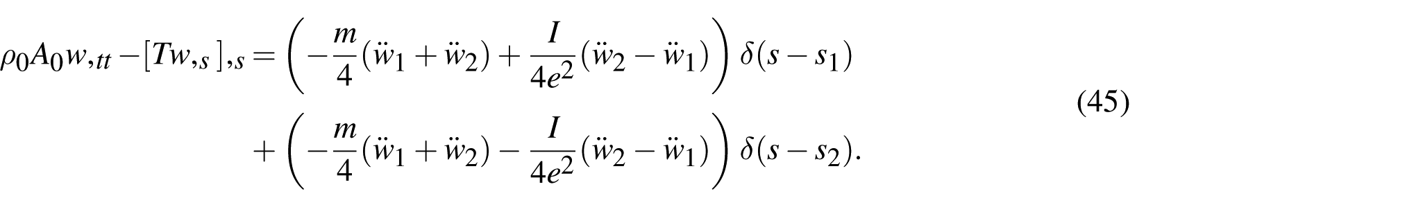
\begin{matrix} ρ_{0} A_{0} g (L_{0} - s) + mg - m a_{m} > 0 for 0 \leq s \leq s_{m} < L_{0} . \end{matrix}

(44)

For this tension and substituting the expressions for reaction forces from equation (42) into equation (6) yields the reduced EOM as

\begin{matrix} \begin{matrix} ρ_{0} A_{0} w,_{tt} - [Tw,_{s}],_{s} & = (- \frac{m}{4} (ẅ_{1} + ẅ_{2}) + \frac{I}{4 e^{2}} (ẅ_{2} - ẅ_{1})) δ (s - s_{1}) \\ + (- \frac{m}{4} (ẅ_{1} + ẅ_{2}) - \frac{I}{4 e^{2}} (ẅ_{2} - ẅ_{1})) δ (s - s_{2}) . \end{matrix} \end{matrix}

(45)

Equation (45) represents the linearized form of the geometrically nonlinear string model considered in [29], obtained under the assumptions of negligible longitudinal displacement and negligible dynamic variation of tension.

The essential boundary condition for a hanging string [44] is as follows

\begin{matrix} w (0, t) = 0 . \end{matrix}

(46)

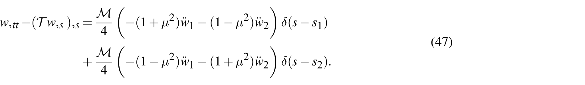
Using the non-dimensional parameters defined in (18), and subsequently dropping the overbars for convenience, the simplified non-dimensional form of the EOM is given by

\begin{matrix} \begin{matrix} w,_{tt} - (T w,_{s}),_{s} & = \frac{M}{4} (- (1 + μ^{2}) ẅ_{1} - (1 - μ^{2}) ẅ_{2}) δ (s - s_{1}) \\ + \frac{M}{4} (- (1 - μ^{2}) ẅ_{1} - (1 + μ^{2}) ẅ_{2}) δ (s - s_{2}) . \end{matrix} \end{matrix}

(47)

where the non-dimensional tension is transformed from equation (43) as

\begin{matrix} T (s, t) = {\begin{matrix} (1 - s) + M - M a_{m} & if 0 \leq s \leq s_{m} \\ (1 - s) & if s_{m} < s \leq 1 . \end{matrix} \end{matrix}

(48)

To evaluate the value of non-dimensional $a_{m}$ , to avoid the slacking in the string, from condition equation (44), we get

\begin{matrix} a_{m} < \frac{1 - s}{M} + 1 for 0 \leq s \leq s_{m} < 1 \end{matrix}

(49)

and the global safe range value of $a_{m}$ correspond to situation when $s = s_{m}$ and $s_{m} \to 1$ in the above condition, we get

\begin{matrix} a_{m} < 1 . \end{matrix}

(50)

In this study, we have considered the scenario of a uniformly moving mass; hence, the string, due to the moving mass, never slackens.

The non-dimensional boundary condition at the end reduces to

\begin{matrix} w (0, t) = 0, \end{matrix}

(51)

while the free end’s displacement is finite.

For the hanging string, we choose the following set of normalized trial functions as

\begin{matrix} W_{j} (s) = \sqrt{2} \sin (ω_{j} s), ω_{j} = (2 j - 1) π ∕ 2 . \end{matrix}

(52)

This set of trial functions introduced above satisfy the essential boundary condition given in equation (51). In addition, the chosen trial functions satisfy the required orthogonality properties (22). Note that one can also choose the eigenfunction of a free hanging string (without moving mass), which is a Bessel function, as the trial functions.

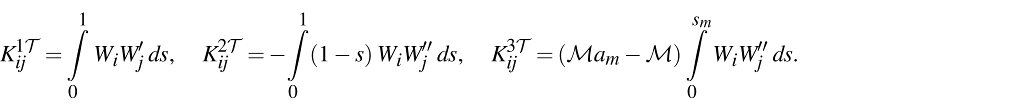
Substituting these trial functions into equation (25) results in the discretized EOM (26). The associated components of mass, damping, and stiffness matrices are defined by equation (28)–(31), respectively. For uniformly prescribed motion of the mass, the relative (prescribed) acceleration vanishes, i.e. ${\overset{\cdot\cdot}{s}}_{m} = a_{m} = 0$ , and consequently the stiffness contributions associated with this acceleration, given by equation (31), do not contribute to the system dynamics. In addition, the stiffness term defined in equation (27) admits a particularly simplified form, as below

\begin{matrix} K_{ij}^{T} = K_{ij}^{1 T} + K_{ij}^{2 T} + K_{ij}^{3 T} . \end{matrix}

(53)

where the coefficient matrices are defined as

K_{ij}^{1 T} = \int_{0}^{1} W_{i} W_{j}^{'} ds, K_{ij}^{2 T} = - \int_{0}^{1} (1 - s) W_{i} W_{j}^{″} ds, K_{ij}^{3 T} = (M a_{m} - M) \int_{0}^{s_{m}} W_{i} W_{j}^{″} ds .

The simplified discretized EOM (26) with $f_{i} = 0$ are integrated numerically as before using a fourth-order Runge–Kutta scheme implemented in MATLAB software.

6.1. Initial condition

Note that the hanging string does not experience external transverse excitation due to gravity. Within the linear formulation, gravity contributes only along the axial direction ( ${\hat{g}}_{1}$ ) that affects the tension in the string and therefore produces no forcing in the transverse direction ( ${\hat{g}}_{2}$ ). As a result, a prescribed axial motion of the mass, $s_{m} (t)$ , does not by itself generate transverse dynamics; the string would remain in its straight equilibrium configuration unless perturbed.

To obtain a meaningful transverse response and to study the transient response of the system, a small initial disturbance must be introduced. In this work, we impose a slight initial rotation of the string about the fixed end as shown by line $O B_{i}$ in Figure 12(a), denoted $θ_{0} = θ (s, 0)$ , chosen to remain within the small-deformation assumption so that $θ (s, 0) \approx \tan θ (s, 0)$ . For engineering purposes, values up to $θ (s, 0) \leq 0.2 rad$ ( $\approx 11 . 5^{\circ}$ ) are acceptable. Note that θ remains the same in dimensional and non-dimensional descriptions.

The generalized coordinates ${p_{j}}$ at $t = 0$ follow from equation (21), and can be computed as follows

\begin{matrix} w (s, 0) = s θ_{0}, \end{matrix}

(54)

hence

\begin{matrix} p_{i} (0) = θ_{0} \int_{0}^{1} s W_{i} (s) ds, i = 1, 2, \dots, N . \end{matrix}

(55)

A higher value of N yields the required straight-line initial condition. The string is released from this small initial orientation $θ_{0}$ , and simultaneously, the moving mass begins to ascend or descend along the string.

6.2. Results and discussions

For the hanging string-moving mass system, we have a total of five parameters: mass ratio $M$ , initial straight configuration of the string making a small angle $θ_{0}$ with ${\hat{g}}_{1}$ , prescribed uniform velocity $v_{m}$ , eccentricity of the contact point from the center of mass e, and factor of gyration μ. In the following, the system’s response is evaluated for different values of these parameters, while keeping $θ_{0} = 0.1$ . For a descending mass, when $e = 0$ , the axial position evolves as $s_{m} = v_{m} t$ , since the mass starts from the origin and moves with a uniform velocity $v_{m} {\hat{g}}_{1}$ . In contrast, for an ascending mass, the position is given by $s_{m} = 1 - v_{m} t$ , as the mass begins at the free end and travels upward with a uniform velocity $- v_{m} {\hat{g}}_{1}$ .

Figure 13 illustrates the convergence of the trajectories of a moving point mass on a hanging string, initially released from an angle $θ_{0} = 0.1$ . The parameters are set to $M = 0.2$ , $e = 0$ , $μ = 0$ , and $v_{m} = 0.1$ . Figure 13(a) presents the convergence behavior for a descending mass, while Figure 13(b) corresponds to an ascending mass. A comparison of the two cases indicates that the trajectory of the descending mass converges more rapidly than that of the ascending mass. The insets highlight the effect of the truncation order N in the Galerkin approximation, revealing subtle differences among the trajectories. For $N = 100$ and $N = 160$ , the trajectories nearly coincide in both ascending and descending cases, indicating sufficient convergence. Based on these observations, a truncation order of $N = 160$ is adopted for all subsequent results, unless stated otherwise.

Figure 13.

Convergence of the trajectories of a uniformly moving point mass on a hanging string for increasing value of N in the truncated Galerkin solution. (a) The different trajectories for a descending mass, and (b) the different trajectories for an ascending mass for parameters $M = 0.2$ , $v_{m} = 0.1$ , $μ = 0$ , and $e = 0$ .

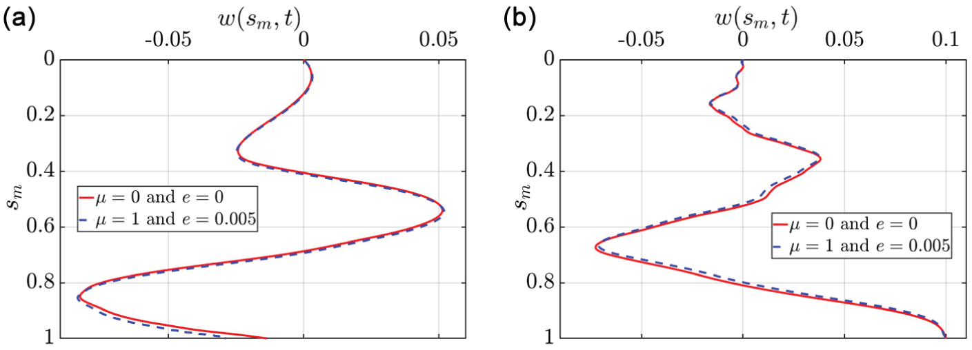
For $M = 0.2$ and $v_{m} = 0.1$ , Figure 14 compares the trajectories predicted by the moving point mass model and the proposed two-point contact model, with $μ = 1$ and $e = 0.005$ . The results show that the two models yield almost identical trajectories. Moreover, unlike the case of a horizontally stretched string with a uniformly moving mass, no noticeable jumps appear at the boundaries for $v_{m} = 0.1$ , indicating smooth and consistent motion for both models.

Figure 14.

Comparison between the trajectories obtained using the moving point mass model and the moving two-point contact mass with rotary inertia (robot). (a) Results for a descending mass; (b) results for an ascending mass. The simulations are performed for $M = 0.2$ and $v_{m} = 0.1$ .

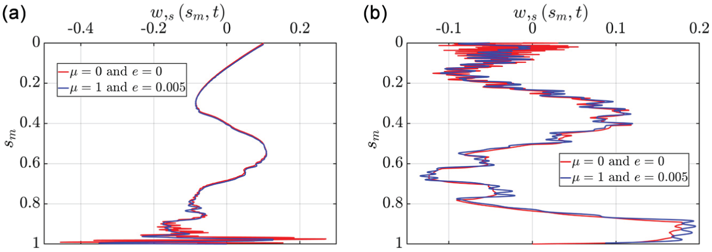
For the same set of parameters, Figure 15 compares the slope at the moving mass predicted by the point mass ( $θ_{m}$ ) and two-point contact models. In both ascending and descending cases, the slope histories show noticeable differences between the two formulations. As the mass approaches the terminating boundary, $B_{t}$ for the descending case and O for the ascending case, the point mass model exhibits a larger slope amplitude than the two-point contact model. A comparison of the slope magnitudes near the free end in Figure 15(a) and near the fixed end in Figure 15(b) indicates that the descending mass produces higher slope amplitudes due to the negligible tension near the free end [45]. In contrast, for the ascending mass, the consistently larger slopes observed during the motion are primarily influenced by the initial configuration of the string.

Figure 15.

Comparison between the slope curves at $s_{m}$ for a moving point mass and a moving mass with rotary inertia (robot). (a) Different slope curves for a descending mass, and (b) different slope curves for an ascending mass for parameters $M = 0.2$ and $v_{m} = 0.1$ .

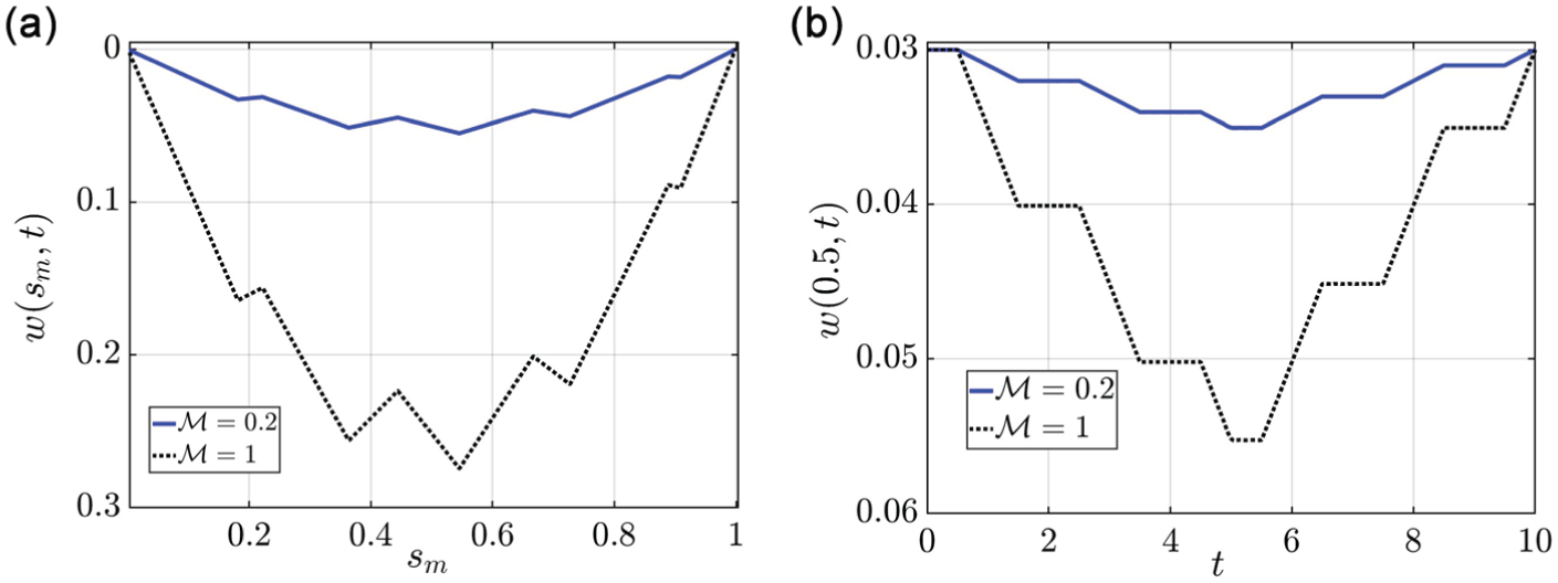
For the moving point mass model with $e = 0$ , $μ = 0$ , and $v_{m} = 0.1$ , Figure 16(a) and (b) presents the trajectories of the mass for different values of the mass ratio $M$ , corresponding to the descending and ascending cases, respectively. In the descending case, increasing $M$ shifts the location at which the transverse displacement of the mass becomes zero to larger values of $s_{m} = v_{m} t$ , thereby delaying each crossing of the mass at the string’s equilibrium position $w = 0$ . Conversely, in the ascending case, a larger $M$ causes the zero transverse displacement of the mass to occur at smaller values of $s_{m} = 1 - v_{m} t$ , which again results in a delayed crossing in time of the equilibrium position during each passage. These behaviors are attributed to inertial effects: a heavier moving mass increases the system’s inertia, leading to greater resistance to motion and a slower dynamic response in both directions of travel. It is also observed that the descending trajectories remain smooth, with no visible jumps near the free end. However, in the ascending case, a jump appears near the fixed end when a heavier mass approaches from the free end, as highlighted in the inset of Figure 16(b). This behavior motivates further investigation of the system at higher mass velocities to examine the potential emergence of trajectory paradox-type responses.

Figure 16.

Trajectories for different mass ratios $M$ . (a) Different trajectories for a descending mass, and (b) different trajectories for an ascending mass for parameters $v_{m} = 0.1$ , $μ = 0$ , and $e = 0$ .

For the moving point mass with parameters $M = 0.2$ , $e = 0$ , and $μ = 0$ , Figure 17(a) and (b) present the trajectories for different values of the relative velocity $v_{m}$ in the descending and ascending cases, respectively.

Figure 17.

Trajectories for different values of $v_{m}$ . (a) Responses for a descending mass; (b) trajectories for an ascending mass. The results are obtained for $M = 0.2$ , $μ = 0$ , and $e = 0$ .

In the descending case, increasing the mass velocity reduces the total non-dimensional travel time, $t_{total} = 1 ∕ v_{m}$ . As a result, the system has less time to respond to the parametric excitation induced by the interaction between the moving mass and the string, causing the trajectory to approach the initial string configuration $w (s, 0)$ at higher velocities. A similar trend is observed for ascending motion: as $v_{m}$ increases, the trajectory of the moving mass tends toward the initial state of the string. However, unlike the descending case, the ascending motion exhibits a noticeable jump near the fixed boundary O at higher speeds, such as $v_{m} = 0.6$ and $v_{m} = 0.9$ . The boundary jump is highlighted in the inset of Figure 17(b). This behavior is consistent with observations previously reported for a horizontally stretched string, even though, in the hanging configuration, gravity does not act directly in the transverse direction as it does in the horizontal case.

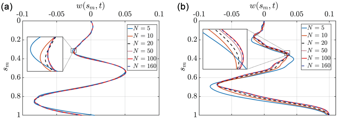
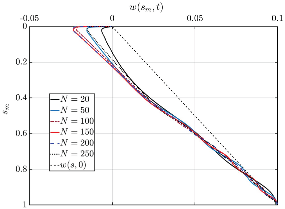
For $M = 0.2$ , $e = 0$ , and $μ = 0$ , Figure 18 illustrates the convergence behavior for the ascending mass trajectories with increasing $N$ . A clear jump (discontinuity) appears near the fixed boundary $O (0, 0)$ as $s_{m} \to 0$ , and convergence in this neighborhood is notably slow. As $N$ increases, the trajectories approach a limiting curve away from the initial string’s state $w (s, 0)$ . However, unlike the stretched-string configuration, where trajectories far from the jump converge and overlap for $N \approx 100$ (see Figure 3(a), away from the terminating boundary $s_{m} = 1$ ), the present case does not exhibit overlapping curves even for larger $N$ . This behavior is attributed to the strong dependence on the initial string configuration and the presence of a non-zero imposed initial condition. These effects become less significant for relatively slow mass motion, for which the trajectory jump is absent; for example, at $v_{m} = 0.1$ , converged trajectories are obtained for both descending and ascending cases, as shown earlier in Figure 13.

Figure 18.

The trajectory for different values of N and $v_{m} = 0.9$ . Jumps in the trajectories are present at this high velocity.

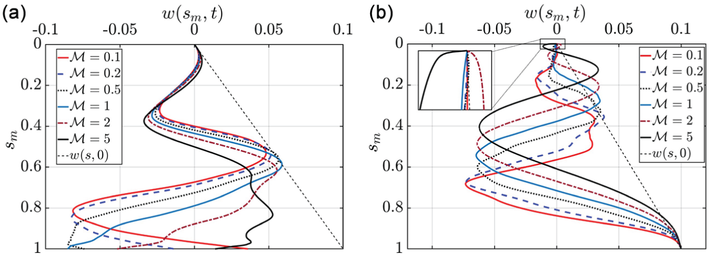
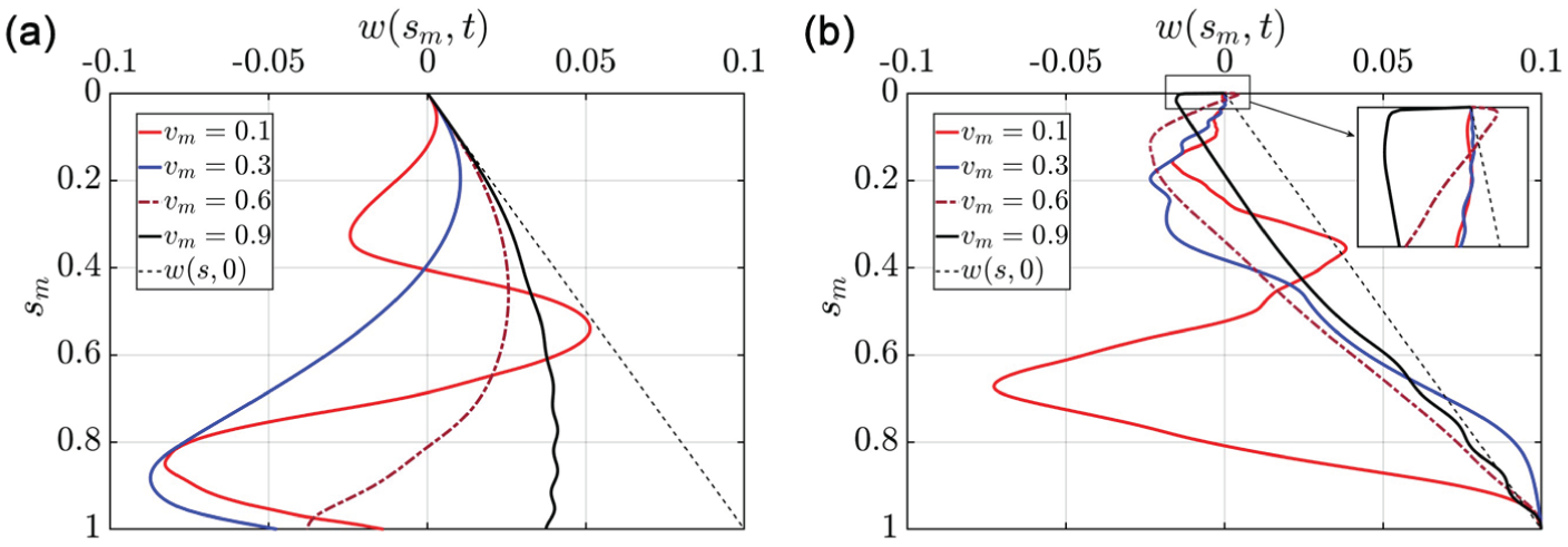
To further investigate these variations using the two-point contact model, Figure 19 presents the actual trajectories for $M = 0.2$ and $μ = 1$ . Figure 19(a) and (b) illustrates the actual trajectories corresponding to different eccentricities e for descending and ascending masses, respectively, at a prescribed velocity of $v_{m} = 0.6$ . For the descending case, the trajectories remain closely clustered across all selected values of e. In contrast, the ascending case exhibits significant separation between trajectories over the entire spatial domain of $s_{m}$ .

Figure 19.

Trajectories corresponding to different values of $e$ are shown. (a) and (b) Trajectories of a descending and an ascending mass, respectively, at $v_{m} = 0.6$ . (c) and (d) Corresponding trajectories for descending and ascending motion at a higher velocity of $v_{m} = 0.9$ .

This behavior differs from that of a stretched string with a moving mass, where a small rotary inertia ( $I = m {(μe)}^{2}$ , see equation (2)) primarily affects the response near the terminating boundary because of the jump characteristics. In the hanging configuration, even a small rotary inertia significantly alters the global system dynamics. Moreover, despite employing the two-point contact model, a pronounced jump in response persists near the boundary O for all considered small values of e.

Figure 19(c) and (d) extend this analysis to a higher prescribed velocity, $v_{m} = 0.9$ , for descending and ascending motions, respectively. In both cases, the trajectories diverge substantially, yielding excessively large displacements for relatively larger eccentricities such as $e = 0.004$ and $e = 0.005$ . This indicates that, at higher velocities, the linearized hanging-string model with a two-point contact moving mass is inadequate for capturing the system response. Nevertheless, as demonstrated earlier in Figure 14, the two-point contact model generally produces stable and convergent solutions with small displacements for a smaller prescribed velocity of the moving mass. Therefore, further investigation of the trajectory paradox in terms of the separation between the actual and virtual centers of mass, or variations in contact-point spacing, would be inappropriate within the present linear framework. Since the formulation is based on a linearized string model, which is valid only for small-deformation dynamics, the large deformations induced by high-velocity two-point contact necessitate a nonlinear modeling approach to properly analyze the transient response, particularly near the terminating boundary.

7. Conclusions

To investigate the dynamics of a linearized classical string interacting with a moving mass, the mass is modeled as a more realistic cable-climbing robot with dual-point contact, engaging the string at two discrete locations. For a prescribed motion of the mass relative to the string, the governing equations are discretized using the Galerkin method and time-integrated via the Runge–Kutta scheme. The developed formulation is then applied to analyze two configurations: (1) a horizontally stretched string subjected to a moving mass and (2) a vertically hanging string carrying a moving mass.

For a horizontally stretched string, the response computed by the present formulation agrees closely with that of a moving point mass away from the terminating boundary. Near the boundary, however, where the trajectory paradox arises in the point-mass model, the two-point contact formulation also exhibits a jump in the trajectory of the front contact. As $s_{2} \to 1$ , the front and rear contact trajectories bifurcate and evolve in opposite directions. A similar divergence is observed between the actual and virtual centers of the moving mass. Furthermore, the rapid increase in separation between the actual and virtual centers, as well as between the two contact points near the boundary, indicates slow convergence of the Galerkin solution in this region. The trends observed with increasing numbers of trial functions suggest the presence of a boundary discontinuity, consistent with the well-known trajectory paradox.

The analysis is then extended to a vertically hanging string carrying a moving mass, considering both ascending and descending motions. Beginning with the moving point-mass model, trajectory convergence is demonstrated in both cases. At higher velocities, the ascending mass exhibits a similar paradox near the upper fixed end. However, in contrast to the stretched-string case, the two-point contact formulation fails to adequately capture the system response for the hanging string, producing excessively large transverse displacements even away from the boundaries, despite having a small rotary inertia. These observations highlight the limitations of the linearized model and motivate the need for further investigation using nonlinear rod theories that incorporate geometric nonlinearities.

Footnotes

Appendix 1 ORCID iDs

Kush Kumar

Shakti S. Gupta

Funding

The authors received no financial support for the research, authorship, and/or publication of this article.

Declaration of conflicting interests

The authors declared no potential conflicts of interest with respect to the research, authorship, and/or publication of this article.

References

Rusin

Śniady

. Vibrations of double-string complex system under moving forces. closed solutions. J Sound Vib 2011; 330(3): 404–415.

Ferretti

Piccardo

Luongo

. Weakly nonlinear dynamics of taut strings traveled by a single moving force. Meccanica 2017; 52(13): 3087–3099.

Luongo

Piccardo

. Dynamics of taut strings traveled by train of forces. Contin Mech Thermodyn 2016; 28(1–2): 603–616.

Frỳba

. Vibration of solids and structures under moving loads, vol. 1. Springer Science & Business Media, 2013.

Smith

. Motions of a stretched string carrying a moving mass particle. J Appl Mech 1964; 31(1): 29–37.

Dyniewicz

Bajer

. Paradox of a particle’s trajectory moving on a string. Arch Appl Mech 2009; 79(3): 213–223.

Gavrilov

Eremeyev

Piccardo

, et al. A revisitation of the paradox of discontinuous trajectory for a mass particle moving on a taut string. Nonlinear Dyn 2016; 86(4): 2245–2260.

Bajer

Dyniewicz

Shillor

. A Gao beam subjected to a moving inertial point load. Math Mech Solids 2018; 23(3): 461–472.

Kumar

Gupta

. Response of a stretched string subjected to a moving mass. Def Sci J 2024; 74(3): 316–320.

10.

Dehestani

Vafai

Mofid

, et al. On the dynamic response of a half-space subjected to a moving mass. Math Mech Solids 2012; 17(4): 393–412.

11.

Markeev

. On stability in a case of oscillations of a pendulum with a mobile point mass. J Appl Math Mech 2017; 81(4): 262–269.

12.

Szyszkowski

Stilling

. On damping properties of a frictionless physical pendulum with a moving mass. Int J Non Linear Mech 2005; 40(5): 669–681.

13.

Chang

Liu

. Dynamic finite element analysis of a nonlinear beam subjected to a moving load. Int J Solids Struct 1996; 33(12): 1673–1688.

14.

Sofi

Muscolino

. Dynamic analysis of suspended cables carrying moving oscillators. Int J Solids Struct 2007; 44(21): 6725–6743.

15.

Ghadiri

Kazemi

. Nonlinear vibration analysis of a cable carrying moving mass-spring-damper. Int J Struct Stab Dyn 2018; 18(02): 1850030.

16.

Yang

Yau

Hsu

. Vibration of simple beams due to trains moving at high speeds. Eng Struct 1997; 19(11): 936–944.

17.

Gladysz

Sniady

. Spectral density of the bridge beam response with uncertain parameters under a random train of moving forces. Arch Civ Mech Eng 2009; 9(3): 31–47.

18.

Rystwej

Sniady

. Dynamic response of an infinite beam and plate to a stochastic train of moving forces. J Sound Vib 2007; 299(4–5): 1033–1048.

19.

Michaltsos

. Dynamic behaviour of a single-span beam subjected to loads moving with variable speeds. J Sound Vib 2002; 258(2): 359–372.

20.

Frỳba

. Impacts of two-axle system traversing a beam. Int J Solids Struct 1968; 4(11): 1107–1123.

21.

Stăncioiu

Ouyang

Mottershead

. Vibration of a beam excited by a moving oscillator considering separation and reattachment. J Sound Vib 2008; 310(4–5): 1128–1140.

22.

Wen

. Dynamic response of beams traversed by two-axle loads. J Eng Mech Div 1960; 86(5): 91–111.

23.

Pisal

Jangid

. Vibration control of bridge subjected to multi-axle vehicle using multiple tuned mass friction dampers. Int J Adv Struct Eng 2016; 8(2): 213–227.

24.

Fafard

Bennur

Savard

. A general multi-axle vehicle model to study the bridge-vehicle interaction. Eng Comput 1997; 14(5): 491–508.

25.

Bajer

Dyniewicz

. Numerical analysis of vibrations of structures under moving inertial load, vol. 65. Springer Science & Business Media, 2012.

26.

Willis

. Preliminary essay to the Appendix b: experiments for determining the effects produced by causing weights to travel over bars with different velocities. Report of the commissions appointed to inquire into the application of iron to railway structures, London, 1849.

27.

Stokes

. Discussion of a differential equation relating to the breaking of railway bridges. Trans Camb Philos Soc 1849; 8(5): 707–735.

28.

Ferretti

Gavrilov

Eremeyev

, et al. Nonlinear planar modeling of massive taut strings travelled by a force-driven point-mass. Nonlinear Dyn 2019; 97(4): 2201–2218.

29.

Ferretti

Piccardo

Dell’Isola

, et al. Dynamics of taut strings undergoing large changes of tension caused by a force-driven traveling mass. J Sound Vib 2019; 458: 320–333.

30.

Henchi

Fafard

Talbot

, et al. An efficient algorithm for dynamic analysis of bridges under moving vehicles using a coupled modal and physical components approach. J Sound Vib 1998; 212(4): 663–683.

31.

Lou

. A vehicle-track-bridge interaction element considering vehicle’s pitching effect. Finite Elem Anal Des 2005; 41(4): 397–427.

32.

Marchesiello

Fasana

Garibaldi

, et al. Dynamics of multi-span continuous straight bridges subject to multi-degrees of freedom moving vehicle excitation. J Sound Vib 1999; 224(3): 541–561.

33.

Yang

Yau

Yao

, et al. Vehicle-bridge interaction dynamics: with applications to high-speed railways. World Scientific, 2004.

34.

Yang

Chang

Yau

. An element for analysing vehicle–bridge systems considering vehicle’s pitching effect. Int J Numer Methods Eng 1999; 46(7): 1031–1047.

35.

Al-Qassab

Nair

O’Leary

. Dynamics of an elastic cable carrying a moving mass particle. Nonlinear Dyn 2003; 33(1): 11–32.

36.

Metrikine

Bosch

. Dynamic response of a two-level catenary to a moving load. J Sound Vib 2006; 292(3–5): 676–693.

37.

Fang

Cheng

. Design and implementation of a wire rope climbing robot for sluices. Machines 2022; 10(11): 1000.

38.

Fang

Cheng

. Advances in climbing robots for vertical structures in the past decade: a review. Biomimetics 2023; 8(1): 47.

39.

Pakdemirli

. Vibrations of a rotating hanged string with a heavy tip mass. Eng Trans 2025; 73(1): 75–87.

40.

Bapat

. An approximate approach to study the free vibration of a string with an arbitrary variation in mass density and tension, with attached concentrated masses, and its application to hanging chain and rotating cord. J Sound Vib 2006; 290(1–2): 529–537.

41.

Novkoski

Fillette

Pham

, et al. Nonlinear dynamics of a hanging string with a freely pivoting attached mass. Physica D 2024; 463: 134164.

42.

Deschaine

Suits

. The hanging cord with a real tip mass. Eur J Phys 2008; 29(6): 1211.

43.

Strichartz

. A guide to distribution theory and fourier transforms. Singapore: World Scientific, 2003.

44.

Hagedorn

DasGupta

. Vibrations and waves in continuous mechanical systems. John Wiley, 2007.

45.

Triantafyllou

. The paradox of the hanging string: an explanation using singular perturbations. J Sound Vib 1991; 148(2): 343–351.

46.

Langer

Klasztorny

. Interpretation of Jakushev’s description of concentrated mass moving along Euler-Bernoulli beam. Arch Civ Eng 1995; 41(1): 5–11.