
Abstract
We have developed a framework that uses multicore CPUs and GPUs found on personal computers to accelerate the computations needed for a class of deformable object modeling algorithms. In recent years there has been a growing interest in using deformable objects in computer applications such as animation, video games, garment CAD, and surgical simulation. Deformable object modeling is quite expensive computationally. However, since most of the related calculations can be parallelized, we have developed a framework that utilizes NVIDIA’s CUDA technology to accelerate a set of deformable object modeling algorithms by transferring their core computations to the GPU. Our results show that frame rates can be improved more than 20 times using GPU compared with using a multicore CPU. In addition, we have developed a method called Local Shape Matching which is an extension to the Shape Matching method. Using this new method we have achieved fast and robust simulations whose implementations have good numerical stability.
1 Introduction
GPUs are becoming a natural platform for computationally demanding tasks in a wide variety of application non-graphical, scientific computation domains. This is due to the increased performance of graphics hardware, and to recent improvements in their programmability.
Even though CPUs have evolved so much and their price has declined significantly, commodity GPUs are delivering better performance with respect to cost for parallelizable computations.
Not only is current graphics hardware fast, but it is growing faster than for CPUs as well. Semiconductor technology, driven by advances in fabrication technology, is increasing at the same rate for both CPU and GPU. The reason that the performance of graphics hardware is increasing faster than that of CPUs is due to the scaled enhancement given by the higher parallelism. CPUs are optimized for high performance for sequential computing; therefore, many of their transistors are dedicated to supporting non-computational tasks such as branch prediction and caching. On the other hand, the highly parallel nature of graphics computations enables GPUs to use additional transistors for computation and capitalize, achieving, higher arithmetic intensity with the same transistor count (Owens et al. 2007).
Owing to the high parallelism that exists in the physical simulation of deformable bodies, we can use the GPU to reduce the calculation time. GPUs have been used for general-purpose computing (GPGPU) for several years. However, since they previously were designed specially for rendering and rasterizing, programmers had to use complicated tricks in order to take advantage of their stream processing architecture. However, efforts has been made to perform the computations of deformable object modeling on GPUs using shaders. Georgii and Westermann (2005) implemented a mass–spring system on GPU. The Nonlinear finite element method has even been implemented on GPU (Taylor et al. 2008). However, since GPU hardware and shaders were not designed for this kind of operation, coding was complicated. NVIDIA’s CUDA 1 (NVIDIA 2008) GPGPU technology is a fundamentally different computing architecture for solving complex computational problems. CUDA supports development using high-level language, further enhancing its popularity.
In the next section we provide background on deformable object modeling and review the literature on their GPU implementation. In Section 3 we explain four methods that are implemented in our framework and introduce a Local Shape Matching (LSHM) method. In Section 4 we explain our GPU-based framework for deformable object modeling. In Section 5 we have shown our results and we have concluded in the last section.
2 Background
In this paper we extend the preliminary study that was presented in Shahingohar and Eagleson (2010) and provide comprehensive results and analysis. We begin by reviewing the literature and motivating our selection of the set of deformable object modeling algorithms that will be implemented comparatively in this paper.
Mass–spring models have been popular in Computer Animation for over 20 years. In SIGGRAPH 87, John Lasseter shocked the computer graphics industry by presenting Luxo Jr. his first 3D animation which was produced at Pixar (Lasseter 1987). His ideas allowed animators to extend traditional 2D storyboarding techniques, keyframe animation, ‘inbetweening’, and scan/print to the 3D realm. At the same venue Terzopoulos et al. (1987) presented the first paper on physically based animation. They employed elasticity theory to construct differential equations to model the behavior of non-rigid curves, surfaces, and solids as a function of time. Since then, many researchers have taken advantage of various scientific concepts, in animation of deformable objects, hair, cloth and fluids (Gibson and Mirtich 1997; Nealen et al. 2006).
2.1 Physically based methods
Most physically based methods for modeling deformable objects are based on continuum elasticity. Under the assumptions of continuum mechanics, the behavior of a deformable object can be expressed as follows. Suppose that the rest shape of a continuous deformable object is a subset of
2.2 Non-physically based methods
Although physically based deformable object modeling methods are generally based on simple continuum elasticity, precise solutions to these methods cannot be implemented in real time. In addition, approximations can make the simulations either very inaccurate, or unstable numerically. Therefore, non-physically based methods that are based on simplifying smoothness constraints are still an attractive choice. The mass–spring method (MSM) and shape matching technique (Müller et al. 2005) are two examples of non-physically based methods. For a complete review of deformable object modeling you can refer to Nealen et al. (2006).
2.3 NVIDIA CUDA and AMD FireStream
In 2006, ATI launched FireStream as the industry’s first commercially available hardware stream processing solution. At first it was designed as a virtual machine abstraction for GPUs that provided policy-free, low-level access to the hardware designed for high-performance, data-parallel applications (Peercy et al. 2006). In the same year AMD acquired ATI and re-branded the API to the AMD Stream Processor, but it was changed to AMD FireStream in 2007. NVIDIA lunched their own GPU parallel computing architecture CUDA in 2007. CUDA gives developers access to the native instruction set and memory of the parallel computational elements in CUDA GPUs. Using CUDA, the latest NVIDIA GPUs effectively become open architectures as programmable as CPUs. CUDA and FireStream both provide similar functionality, however, CUDA seems to have been absorbed by the scientific community. It is shown that typical applications such as traffic simulation, thermal simulation, and
Recently, there has been a growing interest toward cross-platform GPU computation. OpenCLTM is the first open, royalty-free standard for cross-platform, parallel programming of modern processors found in personal computers, servers and handheld/embedded devices. 2 OpenCL is a framework for writing programs that execute across heterogeneous platforms consisting of CPUs, GPUs, and other processors. OpenCL is managed by the non-profit technology consortium Khronos Group and is being developed in collaboration with technical teams at Apple, AMD, IBM, Intel, and NVIDIA. OpenCL is still in its early stages of development but it is highly anticipated that it is going to become the main approach for cross-platform stream processing on the GPU.
CUDA has been used for accelerating some existing deformable object modeling techniques as well. Rasmusson et al. (2008) investigated multiple implementations of volumetric mass–spring–damper systems in CUDA. They compared the performance of CUDA with previous implementations utilizing the GPU through the OpenGL graphics API and showed that performance and optimization strategies differ widely between the OpenGL and CUDA implementations (Rasmusson et al. 2008) The nonlinear finite element method mentioned by Taylor et al. (2008) has been accelerated with CUDA by Comas et al. (2008) within their Sofa Framework.
3 Implemented methods
In this section, we provide an overview of the four methods that are implemented in our framework.
3.1 Weighted MSM
The MSM is the simplest, most intuitive and most common method used in deformable object modeling. Since the early works by Terzopoulos and Fleischer (1988); Terzopoulos et al. (1987) mass–spring method has been used for modeling of various deformable objects such as cloth simulation (Provot 1995; Baraff and Witkin 1998), face animation (Khler et al. 2001) and soft tissue (Gibson and Mirtich 1997; Zhang et al. 2005).
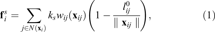
In this system, the deformable object is considered in a discrete space. This model consists of point masses connected together with massless springs and dampers. In the original mass–spring system no weight function is used but we have added weight so nearest neighbors will have a greater effect. By adding weights and considering constant stiffness coefficient
3.2 LSHM
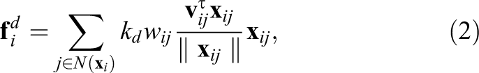
A special meshless non-physically based model for deformable objects was developed by Müller et al. (2005) that is able to provide a robust simulation. We have developed a method for modeling deformable objects based on the ‘Shape Matching’ method. We have extended the concept of clusters in Shape Matching, such that a cluster is defined for each point. An overview of this approach is shown in Figure 1
. At the beginning of the simulation for each node i the center of mass

Local Shape Matching. (a) Node
While rotation can be approximated for each node, we approximate the rotation for the whole shape and use it for all nodes for simplicity. On the other hand, it turns out that we do not have to transform all of the nodes to the rotated coordinate system. The same results can be achieved if we only rotate
{Initialization}
{At each iteration} Approximate the rotation
{Explicit integration}
end for
3.3 Meshless finite element method
If the finite element method is applied to a linear system it produces a linear system of algebraic equations. Assuming linear strain and assuming that our material is isotropic the governing equation of the material (

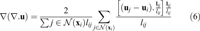
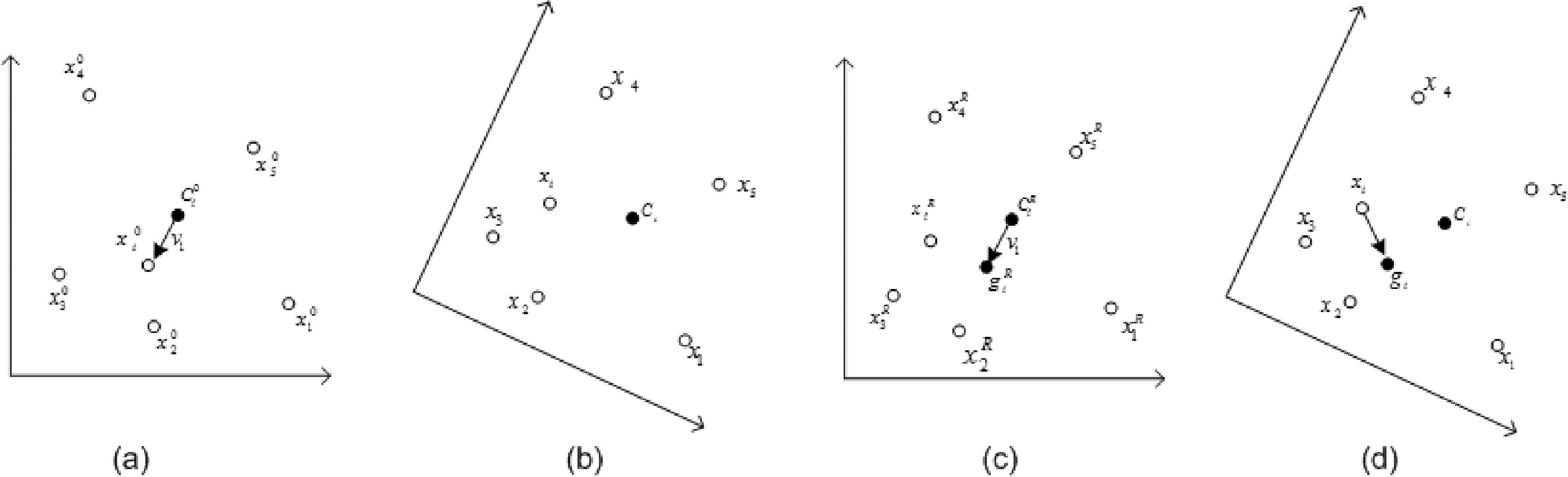
In the original method mentioned all neighbors have the same weight. We have modified this such that closer neighbors will have a greater effect as expected. On the other hand, the original method does not handle significant rotations. In order to fix this, we perform the calculations on the objects coordinate system as we did in the previous section. Therefore, at each iteration we approximate the global rotation of the object. To calculate the Laplacian (Equation (5)) and gradient of divergence (Equation (6)) we need to calculate the displacements (


3.4 Point-based animation
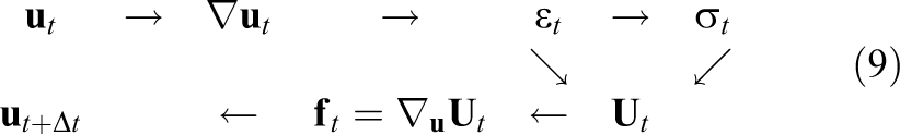
Point-based graphics is an active research area in computer graphics in which the surface is rendered as point sampled surfaces (surfels) rather than polygonal surfaces (Pfister et al. 2000). There has been growing interest in combining mesh-free methods and point-based graphics. Müller et al. (2004) proposed point-based animation (PBA) a mesh-free continuum mechanics method for animation of elastic, plastic and melting objects. In their approach the geometrical strain is approximated around each node based on the deformation of neighbors nodes. Then the derivation of elastic energy is approximated in the area around each point (phyxel) to calculate the resulting elastic force. They use moving least squares optimization to approximate strain, stress and strain energy. To calculate the elastic forces they use the same approach to calculate the derivation of strain energy with respect to displacement. The following is an overview of their method:
4 Our GPU-based framework
We have developed a framework for animating deformable objects based on particle-based methods. Our framework was specifically designed for efficient implementation on CUDA GPU architectures, and can be mapped easily onto other multicore CPUs. An overview of our algorithm is shown in Figure 2 . We made use of the OpenMP (Chapman et al. 2007) library to map the kernel loop onto all available CPU cores. Numerically, we made use of explicit integration and restrict each step to 10 iterations. That means we enforce the boundary conditions only once per 10 iterations which reduces the number of transfers between host and device.
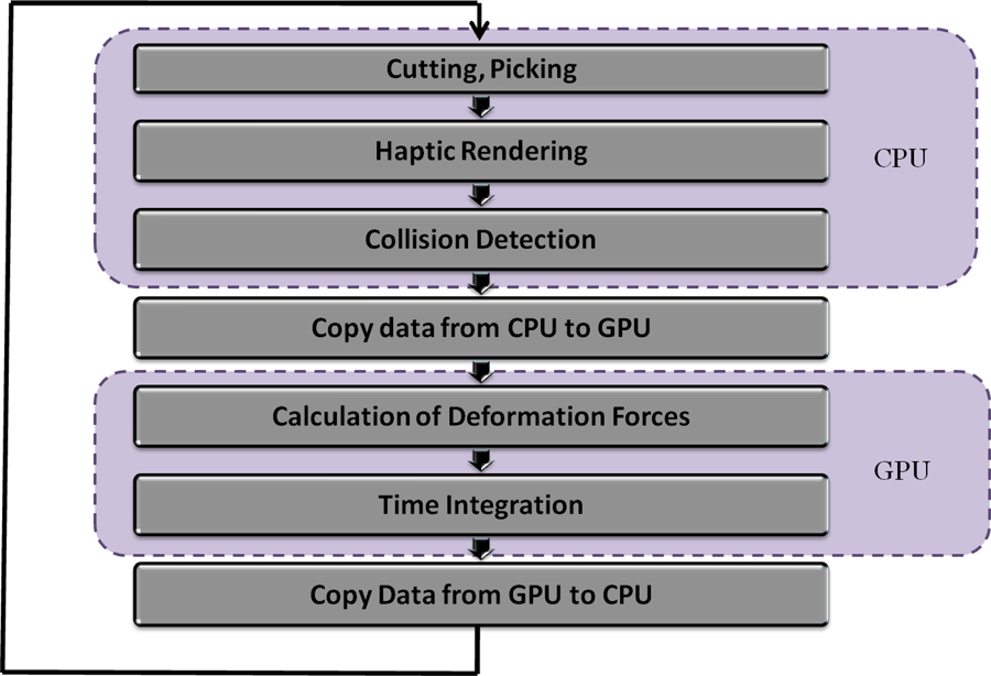
Overview of our simulation framework.
Ideally we want to perform all of the tasks on the GPU; however, some tasks cannot be parallelized and, consequently, they would be even slower on the GPU. Our goal is to utilize the GPU parallel computing capabilities fully by transferring the heavy computation of internal interaction of nodes and numerical integration to the GPU. By doing so, the CPU is reserved for performing sequential tasks such as collision detection.
Transferring data (such as positions of the nodes) between host (CPU side) and device (GPU side) is slow and can easily become a bottleneck for processing. Therefore, we limit these transfers as much as possible.
4.1 Data structure
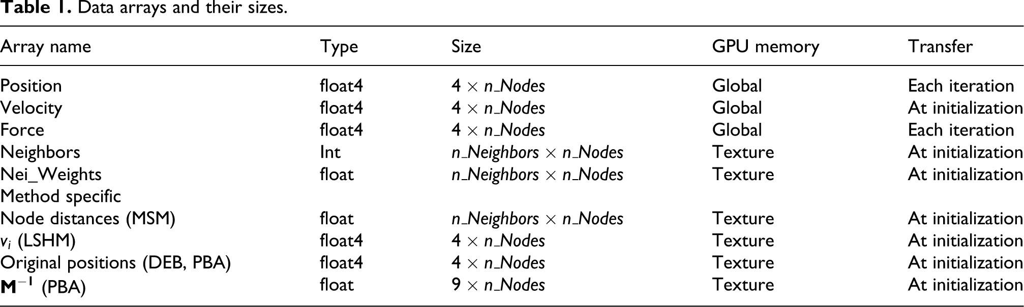
In our framework, for each node a set of arrays are generated to store variables associated with the simulation. These variable are stored for all nodes and include position, velocity, elastic force, list of neighbors, and weight of each neighbor. In addition to these variables, there are others that are specific to each of the methods that we compare, and there fore are declared separately. In the MSM the original length of each spring is stored. One of the features of our LSHM method is that, instead, the vector from center of mass of neighborhood to each node is stored. In the Debunne method only the original positions are saved. In PBA the matrix
Table 1
shows the properties of each variable that is created on the GPU. Velocity, position and force are of float size 4 instead of 3. The reason is that in our CUDA kernel we use float4 since the platform is not optimized for accessing float3.
3
The neighbors array keeps the index of
Data arrays and their sizes.
4.2 Weight function
Different formulas have been used for the weights of the neighbors. Some of these functions are shown in Table 2
. The weight function should be symmetric (
Weight functions used in mesh-free methods (Li and Liu 2007).
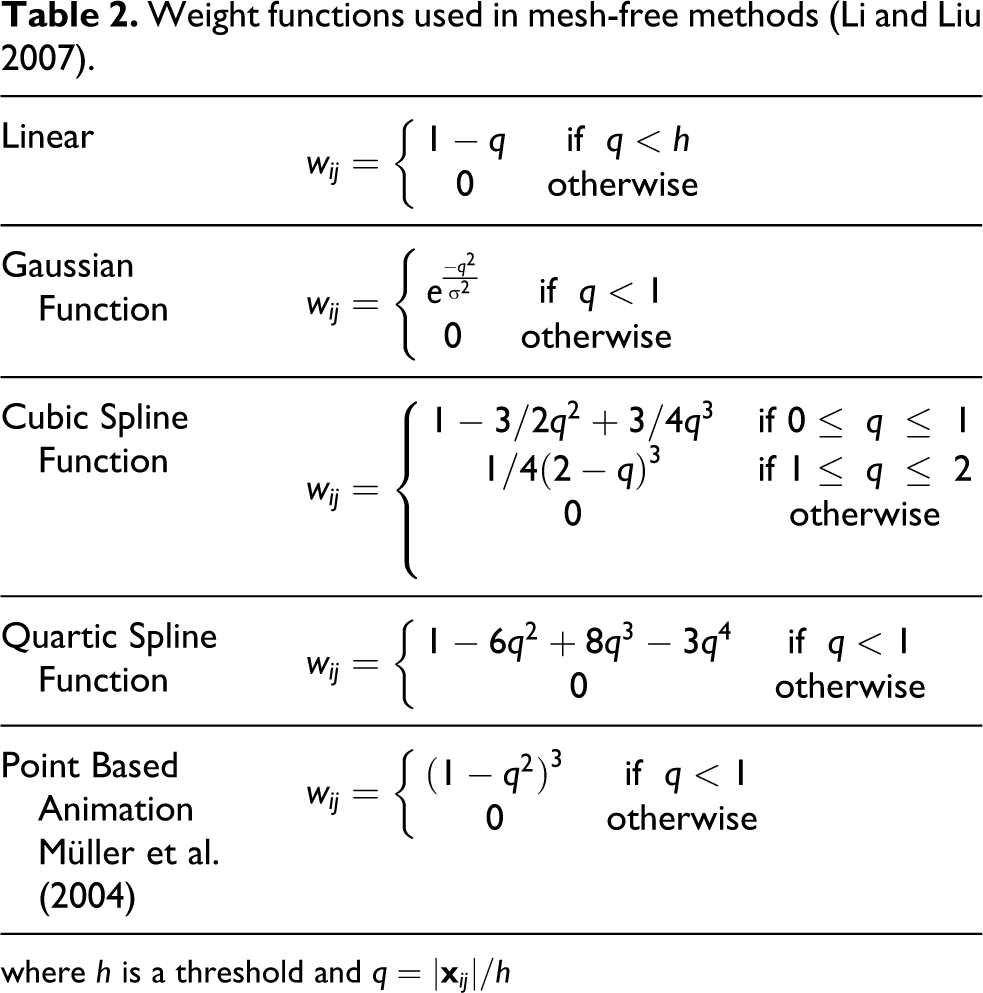
where
5 Results
5.1 Accuracy
In order to compare the accuracy of different methods quantitatively, we have compared our results with the Truth Cube (Kerdok et al. 2003) experiment. Kerdok et al. developed a physical standard to validate soft tissue deformation models. They took CT images of a cube of silicone rubber with a set of embedded Teflon spheres that underwent uniaxial indentation and spherical indentation tests. They used silicone rubber (RTV6166, General Electric Co.) which exhibits linear behavior to at least 30% strain. Two experiments was performed on the Truth Cube. In the first experiment the silicone rubber phantom with embedded fiducial markers (Teflon spheres) was imaged under uniaxial compression. In the second experiment a spherical indentation loading condition was performed. They scanned the experimental setup when the cube was unloaded.
In the first experiment the flat compression plate was held level as it was lowered onto the oiled top surface of the cube to a set displacement. Three loading conditions were scanned: 4 mm, 10 mm, and 14.6 mm displacements producing 5.0%, 12.5%, and 18.25% nominal strain, respectively.
A similar setup was used for the large deformation spherical indentation test except that a 2.54 cm diameter spherical indentor mounted on a 1.9 cm diameter by 4.5 cm long cylinder was added to the compression plate. The first scan was also performed with the cube in an unloaded state for reference locations of the internal spheres. The compression plate with the indentor was then lowered in a manner similar to that of the uniaxial test. Two loading conditions were scanned: 18 mm and 24 mm displacements producing 22% and 30% local nominal strain.
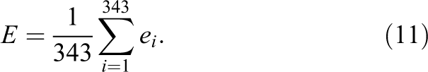
In order to make sure that we track the right positions, we add 343 nodes to each reference mesh. The positions of these additional mesh nodes were initialized based on the position of measured Truth Cube data with zero displacement. In the Truth Cube experiments the cube is in equilibrium state with the presence of gravity force. In other words the stress and strain is not equal to zero from the beginning. For our simulation, we assume that gravity is zero, since if we do not neglect the gravity, our model will deform as soon as the simulation starts, while in the Truth Cube experiment there is no deformation if there is no contact. For the used silicon rubber the Young’s modulus is equal to 15 kPa and a Poisson’s ratio is close to 0.5. In our simulation we have assumed that Poisson’s ratio is equal to 0.499. MSM and LSHM are not based on continuum elasticity, therefore they cannot be expressed by Young’s modulus of elasticity. For these methods the spring coefficient is manually adjusted to achieve reasonable results for those comparisons.
We then simulated the truth cube experiment by lowering a plate to simulate the uniaxial compression test and a sphere to simulate the spherical indentation test. The plate/sphere was moved manually and the position of nodes corresponding to the Truth Cube experiment were saved in a file to be processed later. By comparing the result of our simulation with the Truth Cube we can have a performance measure for linear elastic state. We define a relative error measure for each point as follows: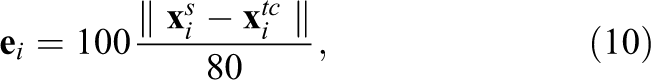
Uniaxial compression
Figure 3 shows the result of simulation of the first Truth Cube experiment on a cube with 2207 nodes with 16 neighbors for each method. The figure shows the results for four strain stages using four different methods. In Figure 5 the error for different combinations of the mesh sizes and number of neighbors are compared together for the uniaxial compression test. The PBA was unstable for the Poisson ratio of 0.49; we were forced to use a Poisson ratio at times as low as 0.40, which causes concern for the applicability of such methods in general. We are pursuing this general modeling issue in our current research.
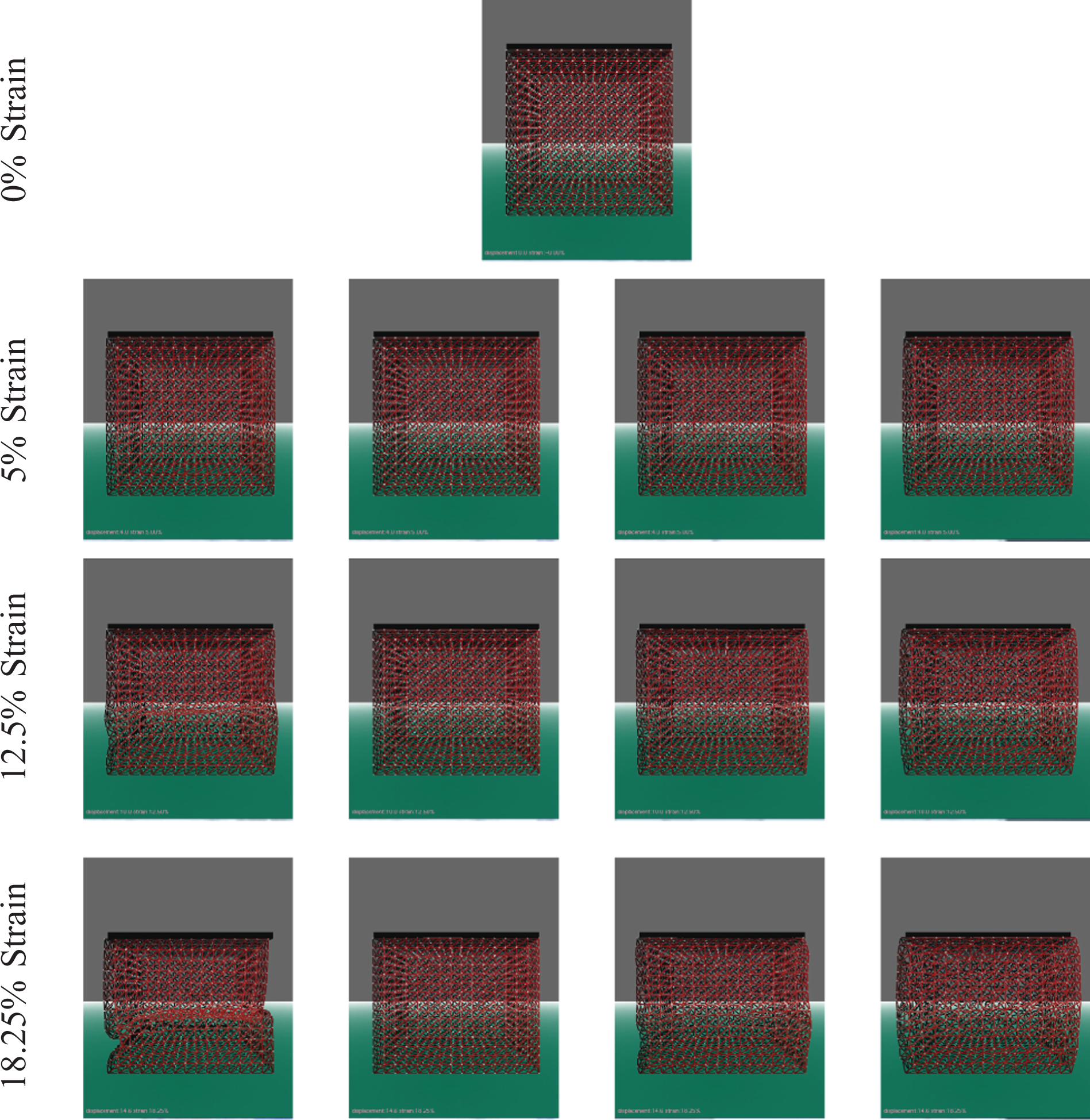
Simulation of uniaxial compression of a cube with four methods in our framework. Number of nodes: 2207; number of neighbors: 16.
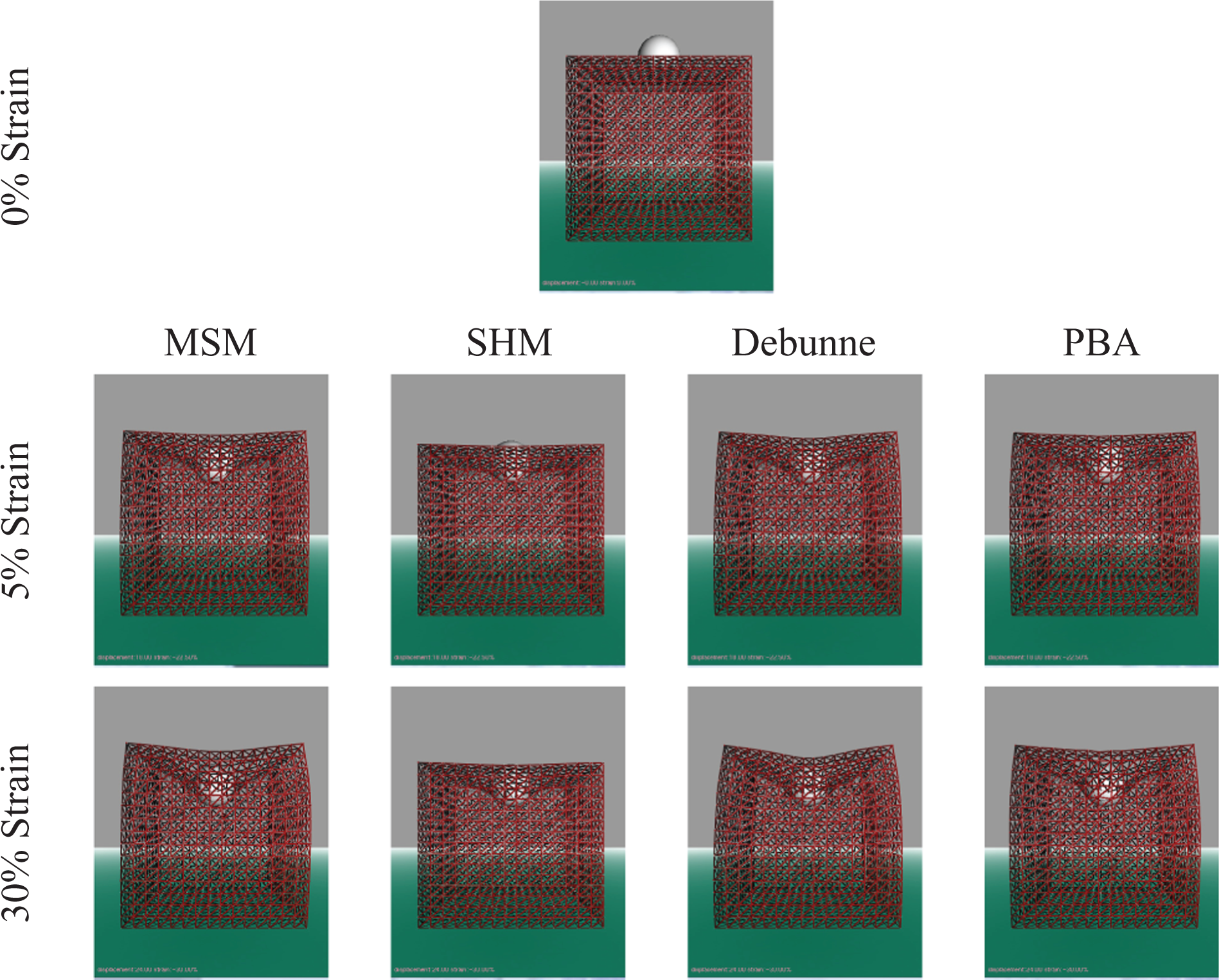
Simulation of the Truth Cube spherical indentation with four methods in our framework. Number of nodes: 2207; number of neighbors: 16.
Accuracy of the simulation in the uniaxial compression experiment.
Spherical indentation
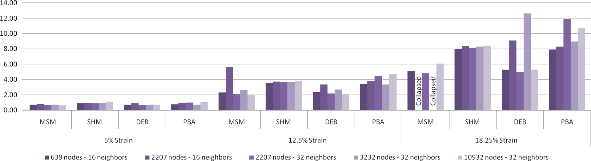
The second experiment has a higher importance for us since it better resembles the interactions in surgical simulation. Figure 4 shows the result of simulation of the second Truth Cube experiment on a cube with 2207 nodes with 16 neighbors for each method. The figure shows the results for three strain stages using four different methods. In Figure 6 the error for different combinations of the mesh sizes and number of neighbors are compared together for the spherical indentation test. Similar to the previous simulation the Poisson ratio of 0.40 was used instead of 0.49 for the PBA.
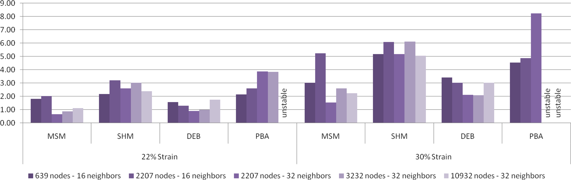
Accuracy of the simulation in the spherical indentation experiment.
Discussion
As we expect the error is higher where there is greater deformation (strain). By manually adjusting the stiffness with trial and error we were able to achieve good results most of the time for MSM, however we had to use different values for different meshes. For example, in the first experiment (Figure 5) for the mesh with 3232 nodes and 32 neighbors although the selected stiffness coefficient has resulted in low error for 5% and 12.5% strain it has resulted in a total collapse in the cube for 18.25% strain. The LSHM method has resulted in lower accuracy compared with MSM since it does not conserve the volume. The error for LSHM is in the same range for all different mesh sizes. This is a desirable feature since it ensures we get the same behavior when the resolution is increased or decreased. The Debunne method has attained lower errors in general; however, it shows sensitivity to the mesh size. Although PBA is the most sophisticated method in our framework it has not acheived the lowest error. This method is suitable for materials with chosen physical properties. As mentioned by Gerszewski et al. (2009) PBA is not appropriate for large elastic deformations. When there is large elastic deformations, using moving least squares for approximation results in ill-conditioned deformation gradient and instability of the simulation. Another reason for instability of this method could be singularity or near-singularity condition in matrix
In general, increasing the resolution of the meshes did not result in improvement in accuracy in all cases. By increasing the resolution of the mesh we have had to increase the number of neighbors to obtain better results. In our simulations, increasing the number of neighbors from 16 to 32 resulted in better accuracy for the mesh with 2207 nodes. In fact we had to use 32 neighbors for bigger meshes to obtain better stability. Another factor that we should take to account is that we have used 32-bit single-precision floating point numbers since our CUDA card did not support DP floating point numbers. That could, potentially, affect the simulations for high-resolution meshes.
It should be noted that the mentioned comparison only provides a measure for linear elastic simulation. Different results might be achieved in the dynamic simulation. On the other hand, in our simulation there was no significant differences between accuracy in CPU and CUDA implementation. As mentioned in Section 4 the boundary conditions in the CUDA implementation is enforced every 10 iterations to get better speed. This might have an effect on accuracy in rapid movements; however, this deficiency is compensated partly in CUDA implementation since time steps will be smaller resulting in a more accurate explicit integration.
5.2 Performance
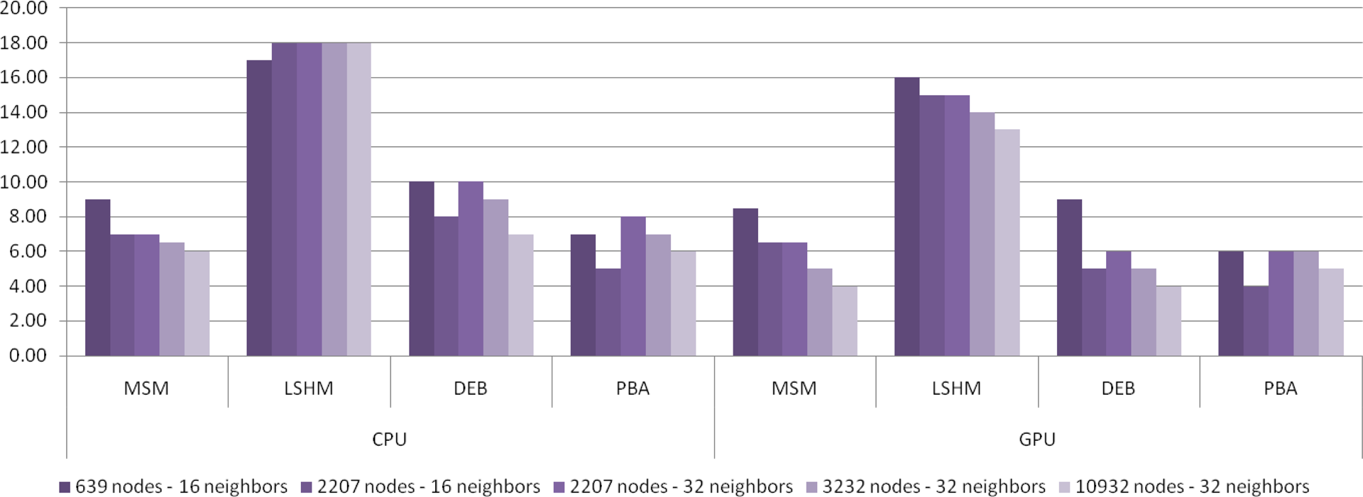
In Figure 8 the calculation time is compared for different implementations. We have used a logarithmic scale to better observe the differences. The simulation is repeated for all four methods for different mesh sizes (639, 2207, 3232, 5567, and 10,932 nodes) and the average calculation time is given in milliseconds when running the algorithm on a single core of a CPU, on four cores of the CPU, and on the GPU. Our LSHM method is faster than any other method since there is no square root operation in its calculations. On a typical processor square root requires 18 cycles while addition, subtraction and multiplication require 2 cycles and division requires 12 cycles.
Stability of the simulation. The bars show the maximum time step (in ms) that can be used without instability.
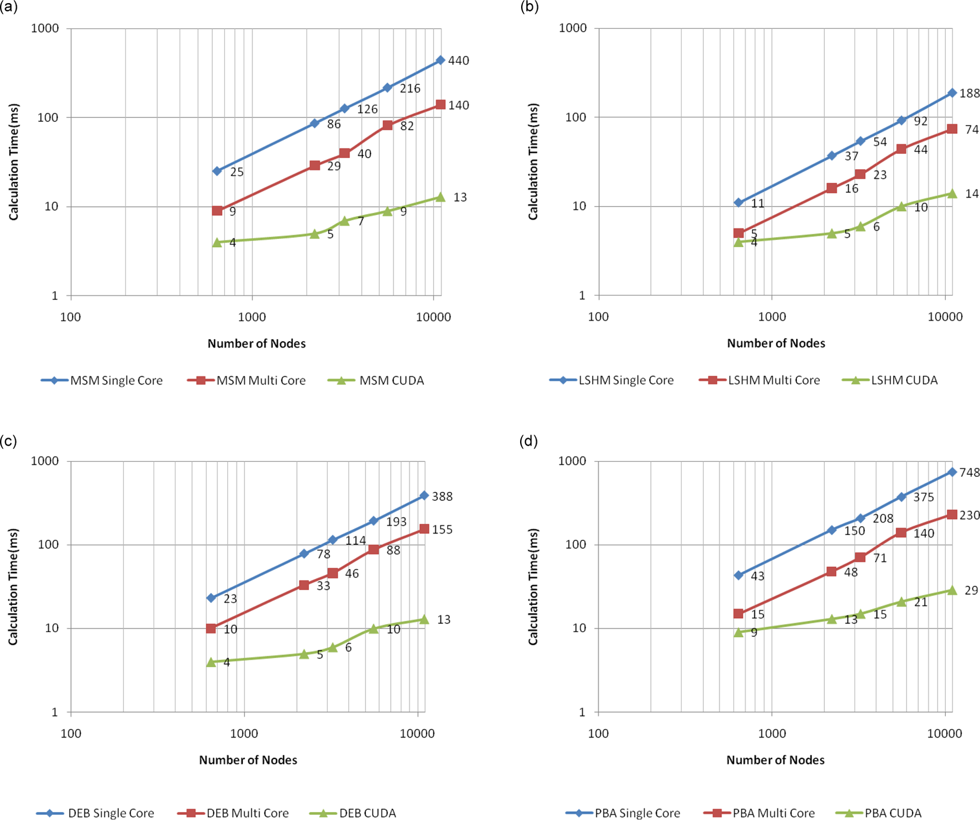
Comparison of calculation time for different methods when 16 neighbors were considered: (a) MSM; (b) LSHM; (c) discretized finite element method (Debunne); (d) PBA.
For all methods the calculation time grows as the number of nodes increases. Using all four cores of the CPU we were able to accelerate the simulation almost three times but it will not be fast enough for real-time applications if the number of nodes is too high. On the other hand by using CUDA we have an acceptable frame rate for all methods even when there are 10,932 nodes. As shown, the slopes of the curves are almost the same for single-core and multicore CPU but CUDA has resulted in a much lower slope for all methods. There is a sudden increase in CUDA calculation time for all methods around 3000. We can conclude that at lower sizes the speed is bounded by the calculation while at higher mesh sizes it is bounded by the bandwidth of the host–device transfer.
5.3 Stability
The explicit integration is not unconditionally stable. Therefore, the time step should be kept low to ensure a stable simulation. In this section we have compared the different methods based on the time step in which they become unstable. For each simulation we started with a small time step and gradually increased the time step until the simulation became unstable. We used the global damping ratio of 0.995 and allowed the simulation to run on a cube which was placed on a surface while gravity was applied. In Figure 7 we have compared the threshold time steps for different methods applied on different meshes. We have also repeated the simulation both on the CPU and the GPU. As is shown, we have been able to achieve the best stability from LSHM. MSM and the Debunne method became unstable at around the same time step. In order to get a better stability in PBA we had to use a Poisson ratio of 0.45 instead of 0.499 that was used in the Debunne method, but the stability is still poor in this method. In general the model has become unstable at lower time steps while using GPU. The reason is that floating point operations are implemented differently on the GPU. The floating point operations have lower accuracy on the GPU than the corresponding operations on the CPU.
6 Conclusion
In this paper we have introduced an efficient framework to implement mesh-free deformable object modeling methods on CUDA. We have shown how deformable object modeling methods can be implemented in this framework. Our framework is more suitable for mesh-free methods; however, simple mesh-based methods such as MSM can be implemented with minor adjustments. Four different methods for modeling deformable objects including the new LSHM method where included in the framework to take advantage of GPU parallel processing. We have shown that while using multicore CPUs the calculation can be accelerated, but it grows with the same rate as a single-core CPU. However, we were able to achieve up to 20 times faster simulations when the number of nodes was more than 10,000. The reason CUDA is faster than CPU is not just having more processing cores, it is also related to the calculation method. When a CPU processing core is waiting for data from the memory it tries to keep itself busy by running awaiting non-dependent instructions out of order; the GPU on the other hand hides the memory loading time by performing the same instruction on other threads.
We have compared the accuracy and stability of the implemented methods in linear static state by comparing the simulation results with the Truth Cube (Kerdok et al. 2003) experiment results. The Debunne method is promising since it results in low errors while it is reasonably fast. LSHM is very fast and robust; however, it results in high errors since it does not conserve the volume. In the future we will add volume-conserving force to this method, to converge towards the desired property of volume preservation in tissue.
Footnotes
Acknowledgement
This work was funded by NSERC operating grant A2630 to RE; and the Canadian NCE on Graphics and New Media, under the HLTHSIM project.