
Abstract
The current generation of graphics cards allows great flexibility in programming. With the introduction of general purpose programming languages for graphics cards, many fields of scientific application will benefit greatly from adapting to this new programming model. Due to the differences in the memory and execution models, not all algorithms can be applied. However, the lattice Boltzmann method can be used to great effect. It allows the simulation of fluids using basic arithmetic operations with a linear complexity, as will be demonstrated. Additionally, the discrete element method can also be adapted to the new model. After outlining the methods themselves and the integration of these two methods into a single simulation, this article will show a way to implement it on graphics cards using the CUDA platform.
Keywords
1 Introduction
In the pharmaceutical industry, medicine is often administered in the form of pills. To produce these pills, a combination of agents has to be mixed in a certain predefined ratio. The mixing process must ensure that these ratios are the same in every single pill, avoiding problems like separating the heavy agents into one half, and the light agents in the other half of the produced lot.
In order to accomplish this, mixing equipment has to be specifically designed to avoid these issues. Currently, this process is done by using existing experience and doing expensive real-world tests. Further applications in this area are outlined by Radeke et al. (2010).
Mixing machinery designed for this application uses rotating blades and air injectors to mix the agents. Powder can be simulated as particles (simplified to spheres in this article). Usually, millions of particles will have to be used to properly simulate the agents, with different classes of particles (differing in size and mass). The injected air lends itself to a fluid simulation, and the rigid parts can be thought of as boundary conditions for both the particles and the fluid.
Current computational simulation research in this area is thwarted by the computational performance currently available. However, the current generation of graphics cards has the potential to overcome this limitation. This means it can be reasonably expected that three-dimensional computational fluid dynamics simulations can be used in a real-time (meaning in this context that the simulated duration is equal to or larger than the computational duration needed) or near-real-time simulation system. This paper demonstrates such a system.
As the Compute Unified Device Architecture (CUDA) technology was invented by Nvidia to simplify the development of these graphics processor-based general computations (GPGPU), it is used in the implementation explained this article. Another option for achieving this goal is the OpenCL standard, which is supported across multiple vendors, but otherwise equivalent. All findings of this article also apply to implementations based on that standard.
As explained in the CUDA programmer’s documentation by Nvidia, the major performance bottleneck in graphics card programming is memory access. Thus, a special emphasis in this article is the memory layout. An even larger issue is transferring data from the computer’s main memory to the graphics processor’s memory, or vice versa. Since the visualization can be done on the graphics processor, no memory copies are necessary for this task. On the other hand, a fluid simulation requires input from a rigid- (or soft-) body physics simulation in order to enable a full dynamic simulation that does not require artificial domain manipulation like creating or removing fluid particles at a specific location. Traditional physics engines like Intel Havok, Nvidia PhysX, ODE and bullet are either fully or partially central-processor-based and thus an integration would require copying the rigid- or soft-body information between the two memory areas (Nvidia PhysX uses the graphics hardware for some of the calculations, but the interface to the application remains on the CPU only, and thus here even two-way copies are necessary). There has been some research on implementing a complete rigid-body simulation (Harada, 2007), so another focus of this article is how to integrate the results of these simulations with the fluid calculations.
The following section delivers a brief overview over the hardware interface of CUDA in order to establish the mindset of developing such a platform. Section 3 introduces the discrete element method for simulating rigid particles, Section 4 explains the fluid simulation and Section 5 expands on this by introducing solid macroscopic obstacles. Section 6 outlines the program flow used in our implementation and Section 7 evaluates it. Section 8 concludes this paper.
2 CUDA
CUDA is an acronym for ‘Compute Unified Device Architecture’, although it is never referred to by its full name. It was invented by Nvidia for their graphics cards, because they saw a large market in applications in general computing that could be accomplished on their device architecture in a much more efficient way than on traditional central-processing units. Before its existence, researchers had to map their problems to graphics-processing tasks like pixel shaders and blend operations.
CUDA allows the implementation of an algorithm in a language very similar to C++, even having source-level integration (interleaving device- and host-functions, using the same data structures and even compiling a function for both at the same time). However, since the graphics card has differing calling semantics, the language had to be adapted. The differences in architecture and the consequences of these differences will be outlined in this section.
2.1 Processor architecture
Unlike traditional processor architectures, graphics cards are designed for parallelization from the ground up.
On a single card, many multiprocessors operate in concert. Traditionally, a single-instruction multiple-data (SIMD) architecture is used to allow commands like vector addition to operate on multiple elements at the same time. The multiprocessors here use a different concept, called single-instruction multiple-threads (SIMT). In this architecture, multiple threads running the same code with partially differing input values are batched together (into a block) and executed. When an arithmetic instruction or a small memory-fetch operation on consecutive memory addresses is to be executed by multiple threads at the same time, these operations are done in parallel (or using a larger memory-fetch operation in the second case). Otherwise, the threads are serialized. Unlike SIMD, this concept allows an arbitrary number of parallel operations to be executed by the hardware, without any adaptations in the program code. Furthermore, it is easier to program, since the programmer only has to handle a single processing unit in a regular linear fashion, parallelization is done automatically where possible.
However, a side-effect is that optimization is harder to do than in SIMD architectures, since optimized operations are not directly visible in the source code. Whenever two threads diverge by going into different code-paths due to branching, the operations cannot be parallelized and thus, performance suffers. Thus, the control flow of these programs should be as linear as possible. The lattice Boltzmann method has this property, as will be demonstrated in Section 4.
3 Discrete element method
The discrete element method (DEM) is an algorithm for calculating the behavior of a large number of particles (usually in the range of 100 000 to millions) together in confined space. It accounts for the velocity and rotation of these particles and aims to simulate the behavior of fluid-like masses like sand, powders and cereals. It is also possible to integrate linear, rolling and radial friction into the collision-handling algorithm.
Note that these particles behave differently to a fluid. For example, the forces between sand particles flowing through a funnel cause the effect used in an hourglass, which is that the flow is constant over time, irrespective of the amount of sand pushing onto the point of constriction. This is not the case for fluids.
It was introduced by Cundall and Strack (1979) for two dimensions and later extended to three. The particles are simplified to spheres, although the model can be extended to other shapes.
The basic idea behind DEM is to use discrete time-steps in the simulation, and assume that the velocity and acceleration between those steps is constant. When choosing a small enough time-step, this assumption causes a negligible error in the results. When two particles collide in the real world, they deform, exerting a force in the direction of the contact. This deformation is simulated by letting the particles overlap. When the collision between two particles can be adequately simulated (meaning that it is within the error tolerances), a domain with many concurrent collisions can be simulated by handling these collisions sequentially (essentially having an atomic time-step, where the collisions happen at once but independently in the simulation). For the mathematical details on how to calculate the forces resulting from a collision, the reader is referred to Radeke (2006).
3.1 The contact list
The tangential overlap
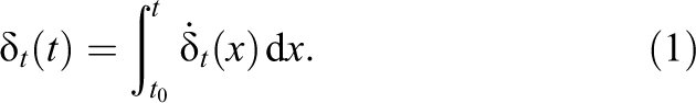
Since the simulation runs in discrete time-steps, the integral has to be replaced by a sum:
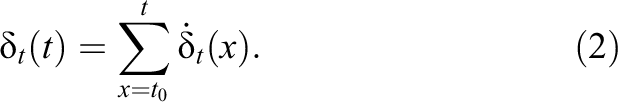
Since it is infeasible to record
This contact list requires a significant amount of space in global memory on the graphics card, which is already used for other aspects of the simulation, like the particles themselves and the fluid simulation. However, we assume that most contacts only last for a single time-step (as is the case in a sparse particle field with few collisions),
3.2 Locating contacts
Locating the contacts in a single simulation step is also non-trivial and thus has to be considered separately.
In order to verify whether two particles with indicies
Using this approach, the naïve solution is to check every possible particle pair using this equation. However, this algorithm has a complexity of
A more efficient approach is to insert the particles into a spatial data structure to eliminate as many potential contact candidates as possible. Since global memory access on GPUs is expensive, the number of read operations has to be kept to a minimum to allow faster operation. The simplest data structure where accessing a location is
Inserting the particles into the data structure has to be done on every simulation step, since particles might move to different cells in a step. Determining the cell the particle belongs to can be done by rescaling the domain to the grid using floating-point arithmetics and then using a rounding operation. Since this operation is efficient, no inter-step spatial correlation effects have to be used to optimize it.
However, since the GPU operates on the data in parallel, the insertion itself is non-trivial. Every cell contains a certain number of ‘slots’ that have to be filled. When one thread is writing into the next free slot, no other thread must access this location. Since there are no global locking mechanisms, this cannot be implemented in that way.
CUDA-capable graphics cards of the second generation and later support atomic operations on global memory. These allow using a usage counter for each field, doing an atomic increment on it. The thread first increments the counter, then writes the particle to the position the counter previously pointed to.
However, NVidia implemented this approach for the CUDA example code called ‘particle’ and came to the conclusion that an alternative algorithm without atomic operations is more efficient. It uses a standard parallelized sorting algorithm provided by the CUDPP library (known as radix sort) instead.
First, for every particle, the cell it shall belong to is calculated (by using the previously mentioned method, and then converting that location to an integer cell index). Then, the particles are sorted by that cell index. For the third step, a separate list is required with the size of one integer times the number of cells, called the cell array. First, this list is initialized to a value denoting that the cell is empty. Then, the sorted particle list is iterated in parallel. In this list, particles belonging to the same cell are next to each other (due to the sorting). Whenever a boundary between two cells is detected (by comparing the current cell index and the cell index of the next particle), the index in the sorted particle array is stored to the cell array at the cell’s location. This way, looking up the particles in a cell requires a lookup in that cell array, and then this index can be used to get the first particle from the sorted particles list, and all subsequent particles, until the cell index does not match any more.
4 Lattice Boltzmann method
The lattice Boltzmann method (LBM) is a numerical algorithm used to solve the Navier–Stokes (NS) equations. It has been demonstrated that it is possible to approximate them directly on a graphics processor using numerical integration schemes (Stam 1999), but in this section it will be demonstrated that a direct mapping of the LBM allows a very efficient and easily comprehensible (and thus, debuggable) implementation, providing a stable basis for a simulation solution.
4.1 The concept behind lattice Boltzmann
The lattice Boltzmann method directly simulates the microscopic fluid particles 1 underlying the macroscopic differential equations of NS. As such, it does not require a solver, but instead, basic iterative mathematical operations.
The LBM can be calculated in both two and three dimensions. The two-dimensional approach is preferable for simulating shallow water in real-time due to the significant reduction of computing and memory requirements. However, since the goal of this article is a physically accurate reproduction of real fluids, the three-dimensional approach is highlighted here.
The domain to be simulated has to be spatially separated into tightly packed cells. Many cell molds are possible, like the dodecahedron (Tolke and Krafczyk, 2008), but the most basic one is the cube, which has been extensively researched, is easily visualizable and will be the focus of this article. Specifically, the D3Q19 geometry is used, since it is the most-researched variant and is a good balance between performance and accuracy.
For an explanation of the equations used in our implementation of the LBM, the reader is referred to Li (2004).
4.2 Initial state
When starting the simulation, the per-cell particle distribution

4.3 Boundaries
Since the simulation domain has to be finite, the boundaries have to be handled. This is problematic on the GPU, since boundaries need special treatment for just the cells at the edge, and branches should be avoided. One way to handle this is to not simulate the cells at the edge, and just set them to constant values. However, this poses issues with byte-alignment on fetching the data (since threads would be off-alignment by one cell with the grid). Our implementation uses the required branches for bounceback boundaries. Since this branch is only executed for a few cells compared to the number of total cells in the whole domain, the thread divergence is not significant and tends towards zero for increasing domain sizes.
4.4 Gravity and external forces
Buick and Greated (2000) outline several methods of varying complexity for integrating external forces like gravity, but the most accurate extends the Bhatnagar-Gross-Krook (BGK) collision operator by another factor:

This external force representation can also be used for interaction with solid macroparticles, which will be explained in Section 6.1.
5 Complex and moving obstacles
In order to incorporate non-cubic containers and other solids like rotors, complex obstacles have to be supported in the fluid simulator. In the work by Monitzer (2008), multiple approaches like the popular one by Mei et al. (2000) were demonstrated, but the approach by Noble and Torczynski (1998) has unique properties that lend themselves well to a GPU-based implementation. Firstly, the modification to the collision step is branch-free, so the performance impact is neglible (at least for the fluid calculation itself, more on that later in this section), and secondly, since a single voxel-based data structure is required for storing the information about the solids, it can easily be stored along with the fluid cells.
For this algorithm, a weighting function
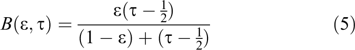
The collision step is modified to include a second collision operator
2

The concept here is that when a solid is in this fluid cell, some fluid particles are unaffected by this solid (as they do not collide with the object), and some are reflected using the no-slip bounceback method. The mixture depends on the amount of solid material in this cell (this was originally designed for porous materials like sand).
Holdych (2003) provides a stable equation (Strack and Cook, 2007) for the bounceback collision operator, which can be simplified to:

As explained by Monitzer (2008, 2010), a disadvantage of this approach is that fully solid cells are still handled as fluid cells. This means that the collision and streaming steps are still applied, even when the collision result is multiplied by
Holdych (2003) proposed a solution to this problem for every cell whose
A fluid fraction
where
The fluid density for these cells is then calculated depending on
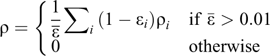
5.1 Improving the voxelization process
Generating the voxel-based data structure for
One approach is to use parametrical representations of the objects immersed in the fluid, and doing an inside/outside determination analytically. However, since the algorithm by Noble and Torczynski (1998) requires knowledge about the volume occupied by the solid in only a single cube, this is non-trivial. One example of this is presented in Section 6.1.1.
A more versatile approach was presented by Eisemann and Décoret (2008). It uses a single-render pass using the regular graphics pipeline with custom shaders to generate a voxelization of the objects, including their interior.
In order to determine not only a binary inside/outside classification for every cell but a density value, Eisemann and Décoret (2008) proposed increasing the voxel density two-fold, and then looking at
Note that thin objects like sheets of paper might cause fluid to trickle through when using sub-voxel precision, since the end result would be
6 Implementation on the GPU using a new data structure layout
NVidia provides sample code for DEM called ‘particle’ as part of the CUDA SDK, which has been optimized for the GPU and so is used as a basis for the implementation described here. The program has been improved by adding the calculation of rotational velocity for the particles, as outlined by Radeke (2006).
When implementing the LBM on a GPU, the first focus should be to look at the data structures used. The following information is known per cell:
The velocity u as a vector
The pressure
The fluid distribution
The solid fraction
All except the velocity can be represented by single floating numbers. In traditional scientific simulations, double precision is used, but this is not supported by the graphics architecture available to the authors (the new Fermi architecture does support it). However, Tolke and Krafczyk (2008) explain how to avoid the downsides of single precision, which has the side-effect of allowing simulation domains that are double the size (since the data structures occupy half the memory) and improving performance, since only half the amount of data has to be transferred for every element.
Since the old data is accessed in parallel while the new simulation data is being written, all data structures have to be duplicated, one collection storing the information of the last step and one storing the information of the new step. After finishing the calculation, the two collections are swapped. This technique is known as flip-flopping.
However,
This technique allows handling the whole operation in GPU memory, so no device-to-host or host-to-device copies are necessary, except for recording the results in permanent storage when necessary (e.g. for replaying the simulation afterwards).
Monitzer (2008, 2010) uses the data structures introduced by Li (2004), which split the distribution values into blocks of four into textures containing red, green, blue and alpha channels (RGBA) in a way to allow implementing bounceback accessing only a single texture. However, since we are using CUDA, the order of the
The streamlined algorithm introduced in this article can be broken down into the following pieces:
In the particle–fluid interaction described above, it is assumed that every particle is exactly in a single cell. In reality, this is not always the case. Thus, a constant 100 (which depends on the grid size compared to the particle size and the time-step size) is introduced, which is used to counteract this discrepancy. A more accurate simulation would have to replace this constant by more accurate calculations, as described in Section 6.1.1.
Note that the outer loop is the basic kernel invocation in CUDA and not an explicit for-loop. Since the streaming and the collision step are integrated into a single kernel, all intermediate values can be kept in processor registers, and so only minimal access to memory is required.
However, GPUs do not employ any caching when reading from or writing to global memory, and so these operations still come with a significant speed penalty. The above algorithm requires a scattered read of 19 float values, which can impact performance in a significant way. As an optimization, when using n arrays each holding one
The final memory layout used in the implementation is shown in Figure 1. It uses a single allocation block to remove unnecessary memory allocation overheads and can easily be addressed using the following function (suitable for both the host and device in CUDA):
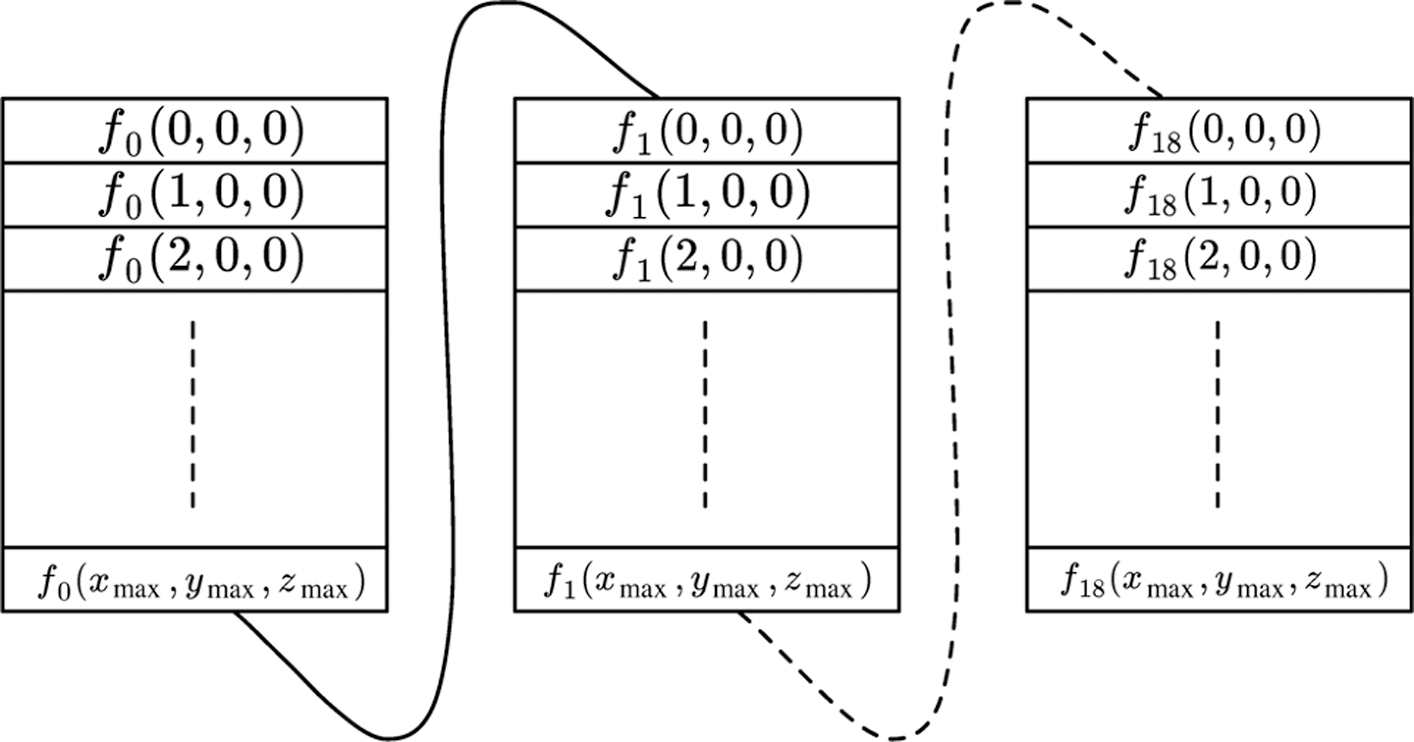
The final memory layout used for the implementation presented in this article. The structure is a single linear array of floating point values. Split into blocks here to improve readability. The dashed lines indicate where elements were left out of the visualization.
The constants dx, dy and dz indicate the grid size in the corresponding dimension. They were stored in constant memory, since they do not change during the lifetime of the application.
Note that two of these arrays are necessary for the flip-flopping technique mentioned earlier in this section.
6.1 Rigid object handling variations
Handling solid objects was explained in Section 5. However, the macroscopic particles used by the DEM primarily require the fluid to apply a force to them, which is not implemented by the solid collision operator. The force could be calculated by taking into account how many fluid particles were bounced back via the
The force of aerodynamic drag is classically defined as
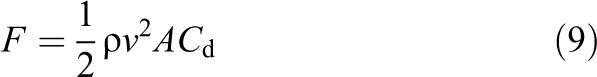
According to Newton, for every force applied there is an equal force applied in the opposite direction. Thus, the interaction between the particles and the fluid can be calculated by taking the force calculated by Equation (9), inverting it and applying it as an external force in Equation (4).
This approach has certain limitations; it only works in this way when every particle interacts only with no more than one fluid cell (the reverse does not have to be the case). However, depending on the lattice size relative to the particle size, it is more likely that a particle overlaps with multiple fluid cells. In this case,
In experiments it was possible to use this drag approach to create a working simulation. However, since every particle only affects a single fluid cell, the force applied to the fluid dissipates too quickly. A workaround is to multiply the force applied by the particle on the fluid by a factor (
6.1.1 Approaching an exact calculation of subcell solid fills
Ultimately, the approach of Noble and Torczynski (1998) is needed for larger solid objects.
The challenge in using this approach is finding the
To calculate the volume of this intersected sphere, it is not possible to use the traditional equations
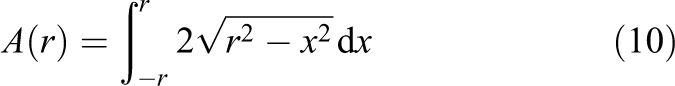
When bounding the integral not to the range
Since the six planes are orthogonal to each other this is a sufficient first step. In the axis orthogonal to the primary axis on the disk’s plane, two more planes (whose distances to the sphere’s origin are denoted by
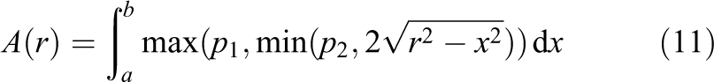
Now the area of the disk (as slice of the sphere) is known, and four of the six planes are taken into account. The general equation for the volume of a sphere is
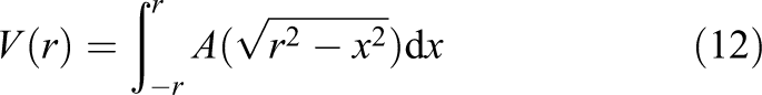
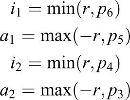
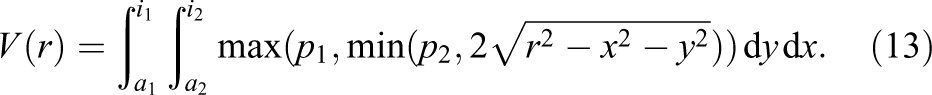
As this approach has a non-continuity due to the
These intersection volumes would have to be calculated for each particle intersecting the fluid cell, added up and then divided by the volume of the cell (
7 Results
Time measurements were done using the Linux-specific function clock_gettime. The first 4000 simulation steps are skipped, then 1000 steps are measured and then the average is printed out. This is done to avoid taking the overhead of the initial configuration into account, which randomly distributes the DEM particles in the domain, thus causing a non-predictable number of collisions.
Only the time difference between the two update methods is measured, so the rest of the application is included in these figures, including visualization.
The testing equipment used was an Intel Core2 Quad running at 2.83 GHz on Ubuntu Linux with a Nvidia GeForce GTX 295 (also running the display) with 896 MB RAM. The application was compiled in 64 bit mode for CUDA 2.3.
Different domain sizes and particle numbers were tested, the results are shown in Table 1. The visual result can be seen in Figures 2 and 3.
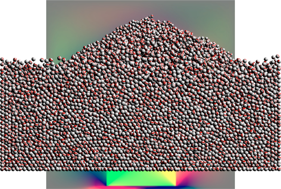
The implementation simulating a
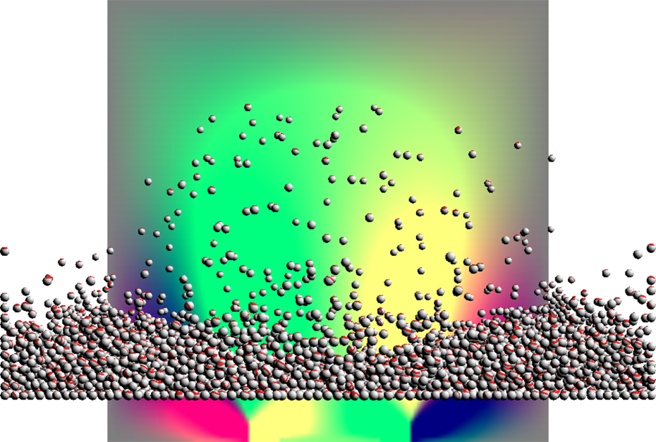
The implementation simulating a
The measurement results. The top row shows the number of particles, the leftmost column shows the fluid and particle domain size. The results are in milliseconds per simulation step.
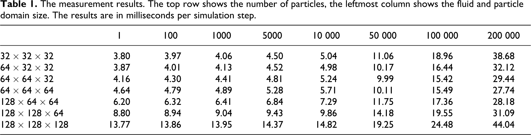
Since there are two simulations with different behavioral patterns mixed in the simulation, a non-monotonic behavior can be seen. On the one hand, the fluid simulation processes every cell of the domain independently, so the number of cells directly influences the performance. On the other hand, the particle simulation does not process every cell, it only processes every particle. For every particle, all other particles in neighboring cells have to be iterated, which means that a larger number of cells, but with a smaller cell size (and thus, fewer particles per cell), reduces the amount of computation required. Thus, measurements with a single particle were carried out, in order to profile the LBM implementation without influences from the DEM code (since no collisions are possible with a single particle, and no neighbors have to be iterated), still keeping the memory and inter-simulation overhead.
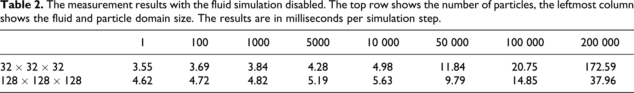
Additionally, the DEM simulation without the LBM simulation was profiled, which can be seen in Table 2. Here, only the simulation call itself was removed, the memory layout and initialization code remain the same. Note that the two tables cannot be directly compared, since without the fluid, the particles fall to the bottom of the domain in a faster fashion and so there are more contacts than when also using a fluid simulation.
The measurement results with the fluid simulation disabled. The top row shows the number of particles, the leftmost column shows the fluid and particle domain size. The results are in milliseconds per simulation step.
7.1 Interpretation
The graphical representations for the combined simulation can be seen in Figures 4 and 5. The performance penalty for an increasing number of particles is non-linear, as can be expected (since the number of contacts increases non-linearly, which is a defining criterion for the performance of a DEM implementation). Of special importance is that a small domain is faster for a small number of particles, but this advantage is reversed when the number of particles increases.
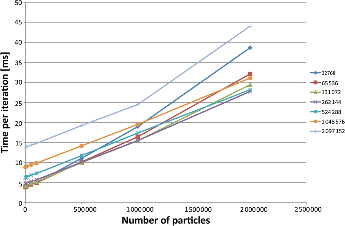
The measurements from Table 1 displayed as a linear plot. The horizontal axis is the number of particles, the vertical axis is the execution time. The cell counts are shown in the legend.
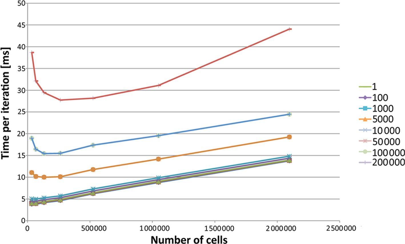
As can be seen in Figure 5, as the number of particles increases, the non-linearity increases. This stems from the fact that the LBM performance is linear to the number of cells. As before, this figure also shows that a smaller domain with a large number of particles hinders performance.
In terms of scaling to larger domains, Figure 6 shows that the number of cells per unit time is logarithmic. However, the memory limit is more important in this regard, as all of the simulation data has to be stored in the graphics memory, and larger domains than
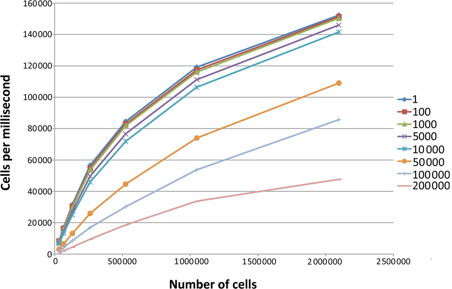
The measurements from Table 1 transformed so that the number cells per millisecond is shown as a measure of performance. The particle counts are shown in the legend.
Figure 7 displays the same information for the simulations with the LBM step turned off. It displays the same trend in a more pronounced fashion, which stems from the fact that the linear time increase of the LBM is removed.
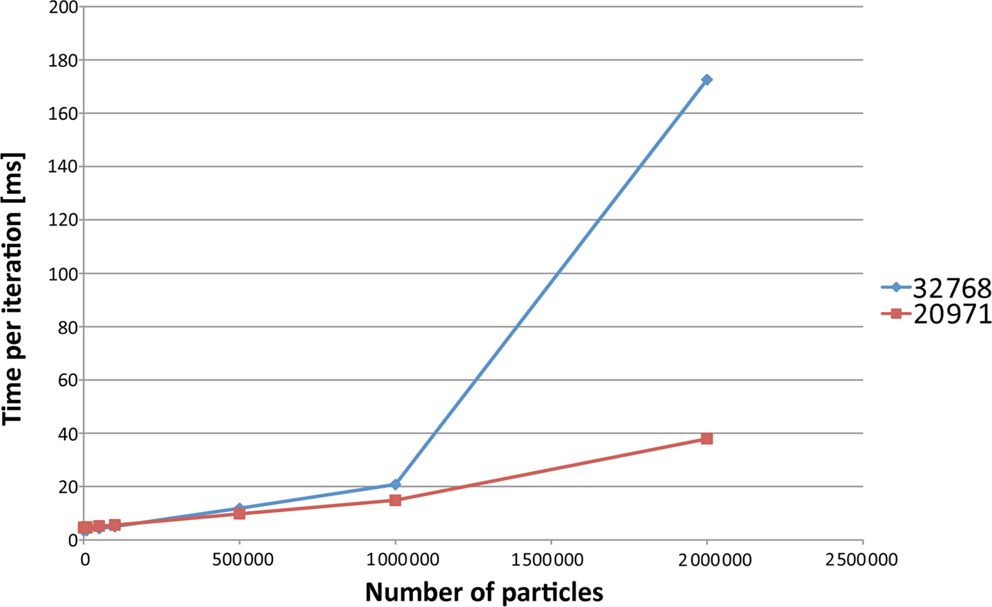
The measurements from Table 2 displayed as a linear plot. The horizontal axis is the number of particles, the vertical axis is the execution time. The legend shows the number of cells.
8 Conclusion
It has been demonstrated that combining a DEM simulation with an LBM simulation is possible using standard methods from both scientific fields, with a simple interface between them. This allows a full physics simulation on a graphics processor, reducing the data transfer necessary between the host and the graphics card, which is usually the limiting factor for graphics processor performance.
The LBM implementation was improved compared to the implementation by Monitzer (2008, 2010) by leveraging the thread scheduler’s optimization capabilities in the area of memory access patterns. Furthermore, a simplified solid interaction model was implemented, which removes the requirement for an expensive voxelization process. Additional options for integrating more accurate interactions were explored. A full implementation was shown and explained, which demonstrates that the LBM is easily integrated into the CUDA model.
As was demonstrated in Section 7, the LBM simulation time increases linearly with an increase in domain size, while the DEM simulation exhibits a global minimum, which depends on the number of particles. A split between the cell size of the LBM and the DEM is therefore recommended, in order to achieve optimal performance for both simulations.
Footnotes
Funding
This research received no specific grant from any funding agency in the public, commercial, or not-for-profit sectors.