A novel approach to train random forests on GPU for computer vision applications using local features

Abstract

The random forests (RF) classifier has recently gained momentum in the computer vision field, thanks to its successful application in human body tracking, hand pose estimation and object detection. In this article, we present a novel approach to train RF on a graphics processing unit (GPU) for computer vision applications where simple per-pixel features are computed. Besides leveraging the processing power of the GPU to accelerate the training, we reformulate the training problem to limit costly image transfers when it is not possible to store the entire data set in GPU memory. Furthermore, our implementation supports arbitrary image types and allows the user to specify custom features. We extensively compare our approach with the state of the art on publicly available data sets, and we obtain a reduction in training time of up to 18 times. Finally, we train our implementation on a large data set (around 100 K images), demonstrating that our approach is suitable for training RF on the vast data sets typically used in computer vision.

Keywords

Random Forests GPGPU computer vision local features image segmentation OpenCL

1. Introduction

The Random Forests (RF) classifier (Breiman, 2001) is an ensemble of decision tree predictors trained on a randomly sampled subset of both the training set data and the feature space. Among the main strengths of RF are a low generalization error, robustness to noise and ease of implementation.

In recent years, RF have been widely adopted in the field of computer vision (CV). Their gain in popularity is mostly due to the work of Shotton et al. (2011) in the context of marker-less full-body tracking. Starting from the images acquired from a Microsoft Kinect sensor, the authors combine the RF with simple per-pixel local features and achieve remarkable results in terms of both accuracy and real-time performance. The same approach was previously applied to object class segmentation (Schroff et al., 2008) and has been further extended to hand pose reconstruction (Keskin et al., 2011), face tracking (Kazemi et al., 2014) and semantic mapping (Stuckler et al., 2012).

Although RF can easily perform prediction in real-time, the training phase usually represents a heavy computational burden. This is especially true in CV applications that use local features since the processing must be performed per pixel on potentially vast training sets (e.g. 1M images in Shotton et al., 2011, around 100 K images in Keskin et al., 2011 and 10 K images in Kazemi et al., 2014). Despite the computational requirements of this phase, it is possible to reduce training time significantly by leveraging the intrinsic parallelism exposed at different granularity levels. Singular trees of the ensemble can be processed in parallel. Furthermore, if the training is performed in a breadth-first fashion, computation on every node at the same tree level can be carried out independently.

Graphics processing units (GPUs) represent an ideal platform for the implementation of RF training. Initially conceived as accelerators for computer graphics (CG) applications, they have evolved into general-purpose processing units with thousands of cores capable of throughputs of the order of teraFLOPS. Thanks to the availability of higher level frameworks (e.g. Nvidia CUDA (NVIDIA Corporation, 2015) or OpenCL (Khronos Group, 2015), existing applications can be easily ported to the GPU, allowing full exploitation of their potential.

To achieve high throughputs on the GPU, two main conditions must be satisfied: workload parallelization and minimum transfers to/from the GPU. The former is a product of the original field of application of GPUs; since in CG the same operations are performed independently and simultaneously on thousands of vertices or pixels, GPU cores are designed to execute the same instructions in parallel on thousands of data elements. Data transfers to/from the GPU are a costly operation because of the limited bandwidth of the PCI bus used to communicate with the CPU: while GPU-dedicated memory bandwidth is of the order of hundreds of GB, third-generation PCI bandwidth is limited to a maximum of 16 GB/s. Therefore, to reduce the communication overhead, it is fundamental to minimize data transfers and to keep data in the GPU as long as possible.

Parallelization on GPU can be exploited at different granularities during the RF training; different trees of the ensemble can be trained in parallel as well as single nodes within the tree. Furthermore, in CV applications, visual features can be extracted in parallel from each image. While training parallelization can be easily achieved, it is not trivial to reduce data transfers, especially in the context of CV applications, where the training set size potentially reaches the order of hundreds of thousands of images. Since GPU’s main memory capacity is not usually sufficient to store the whole training set, images need to be continuously transferred through the PCI bus and the overhead of data transfers to the GPU potentially outweighs the computation time.

We present a novel approach to train RF on GPU for CV applications that require large training set and local per-pixel features. The main contributions of our work are as follows:

we train RF trees on the GPU in a breadth-first fashion with a per-image granularity. This allows reduction in the overhead of moving images to the GPU since only one transfer per image is performed for each tree level.

we compare the performance of our method with the state-of-the-art implementation on publicly available data sets, achieving a speed-up factor up to 18 in the training phase while keeping comparable classification accuracy.

we apply our implementation on a large data set of 100K images and train a single tree in less than 1 day. To the best of our knowledge, this is the first RF implementation able to work on data sets of such size without resorting to distributed systems and using only a consumer-grade GPU.

we released the source code of our implementation Padenti, 2015)¹ with an open-source license LGPL, allowing other researchers to reproduce our experimental results and further improve/extend the features of our RF implementation.

The article is organized as follows: Section 2 provides some background about RF, their application in CV and the state of the art of RF implementations on GPU; Implementation section Section 3 describes our implementation in detail, and finally, section 3 presents a comparison with the state of the art and analyses the performance of our approach in terms of both training time and accuracy on various data sets.

2. Background

2.1. Random forests

We provide a brief introduction to the RF classifier by considering only binary decision trees. A detailed analysis can be found in the work by Criminisi et al. (2012).

2.1.1. Prediction

Given an input datum x and a set of classes $C$ , the RF prediction aims at finding:

c^{*} = \underset{_{c \in C}}{argmax} P (c | x),

(1)

with $P (c | x)$ the posterior probability for class c, given the input datum x . Each tree intermediate node is associated with a split function:

f_{θ} (x) \leq τ

(2)

parameterized by a feature vector θ and a scalar threshold τ. Starting from the root node of a single RF tree T, the split function f is applied to the current datum x and compared with the node threshold τ. Based on the comparison result, the datum is forwarded to the left or the right child node. The comparison and forwarding are repeated until a leaf node l is reached, where the probability $P_{T} (c | l)$ over classes $C$ is stored. This operation is further repeated for each tree of the forest, and the final posterior probability distribution is given by the average of the probabilities of the reached leaves:

P (c | x) = \frac{1}{| T |} \sum_{T, l} P_{T} (c | l) \forall c \in C

(3)

where $T$ is the set of RF trees.

In the context of CV application based on local features, the input datum x is represented by a single image pixel, while f is a function that generally works on the colour values of the current pixel or its neighbourhood. The RF prediction for a single image is illustrated in Figure 1.

2.1.2 Training

Given a training set $D$ of labelled data (i.e. whose classes are known a priori), each tree of the RF is trained on a different randomly sampled subset $S \subseteq D$ . Starting from the root and for each intermediate node of the tree, the training phase searches the more discriminative feature/threshold pair, that is, the tuple $(θ, τ)$ which maximizes a certain score function. The information gain I is usually used and it is defined as:

I = H (S) - \sum_{i \in L, R} \frac{| S_{i} |}{| S |} H (S_{i}),

(4)

where $S_{L}$ and $S_{R}$ are the subsets originated by the application of the split function with the current feature/threshold pair to all the samples in $S$ , and $H$ is the Shannon entropy computed with respect to the classes. For each node n, different subsets $θ_{n}$ and $T_{n}$ of the whole feature and threshold spaces are sampled and the pair that maximizes the information gain is kept. This procedure is applied recursively on the left and right child nodes (depth-first training) or on the next node at the current level (breadth-first training).

The training recursion stops when some termination criterion is met (typically a maximum depth is reached or a node does not receive enough samples), in which case the current node l is marked as leaf and the probability distribution over the classes is computed as:

P (c | l) = \frac{| S_{c} |}{| S |} \forall c \in C,

(5)

with $S_{c}$ the data samples of class c that reached the leaf node.

2.2. Visual features

In the literature, many local features have been proposed for object class segmentation. Some examples are shown in Figure 2. Given a colour image $I$ and a sampled pixel at coordinates x (Schroff et al., 2008), the feature $f_{θ} (x)$ is defined as the following:

f_{θ} (x) = \frac{\sum_{p \in R_{1} (x)} ϕ_{1} (p)}{| R_{1} (x) |} - \frac{\sum_{p \in R_{2} (x)} ϕ_{2} (p)}{| R_{2} (x) |}

(6)

where $R_{i}$ is a region of the image at position $x + x_{i}$ of width $w_{i}$ and height $h_{i}$ , while $ϕ_{i}$ represents a single channel of the image $I$ . The set of parameters $x_{i}$ , $w_{i}$ , $h_{i}$ and $ϕ_{i}$ for the two regions $R_{1}$ and $R_{2}$ forms the feature vector θ.

In the work by Stuckler et al. (2012), the feature of equation (6) is extended by incorporating information from an additional depth channel. Image regions are extracted either on colour or on depth channels. Position offset $x_{i}$ , regions width $w_{i}$ and height $h_{i}$ are both divided by the depth value at current pixel coordinates x to make the feature invariant with respect to depth and translation.

The work by Shotton et al. (2011) applies a simplification to the previous features to address the problem of human body parts segmentation from single-channel depth images:

f_{θ} (x) = I (x + \frac{x_{1}}{I (x)}) - I (x + \frac{x_{2}}{I (x)}) .

(7)

Image regions are replaced by single pixels to allow for better performance, while normalization by the depth value $I (x)$ yields again depth and translation invariance.

These simple features are not sufficient to discriminate between, respectively, object classes and body parts, but their combination with the RF framework allows prediction of the class with which each pixel is associated with good accuracy.

Due to the large number of feature parameters, precomputation of feature responses for all the training set samples (i.e. sampled image pixels) is not feasible. For this reason, the features are computed on the fly when needed by the training process.

2.3 GPU programming model

Recently, various standards for general-purpose computation on GPU (GPGPU) have emerged. Two of the most notable examples are Nvidia Compute Unified Device Architecture (CUDA) and Open Computing Language (OpenCL). In our work, we preferred the latter due to its broader vendor support. Here we briefly present the high-level abstraction exposed by the OpenCL standard (see Munshi et al., 2011, for further details).

OpenCL defines a high-level abstraction of the supported platforms in which the host is responsible for the external communication to the OpenCL environment (e.g. application programs and I/O), and it is connected to one or more compute devices, each of which consists of several compute units responsible for the actual computation. Host and compute devices are typically the main CPU and the GPU, and they communicate via one or more command queues.

The execution model (Figure 3) follows a single program multiple data paradigm, where the application code, defined by a kernel function, is executed in parallel on various streams of data. The execution is performed in lockstep mode, and the same instruction is executed by all the compute units on different data. Each executing kernel instance is known as a work item and is associated with a global ID. Work items can be grouped into work groups. Inside a work group, each work item is identified by a unique local ID. A pool of general-purpose registers is distributed among all the work items to constitute their private memory. Furthermore, all work items of the same compute device share a high-capacity global memory, while a smaller and faster local memory is shared by all work items within the same work group.

To maximize the throughput, it is fundamental to follow specific programming practices, for example, by providing enough work to the compute device to keep all the processing units occupied, by preferring the use of shared memory instead of global memory and by limiting data transfers to/from the GPU. The latter will be fundamental in our implementation to decrease the total time required for RF training.

2.4 Related work

In Sharp (2008), a pioneering work in the implementation of RF on GPU is presented. The author accelerates both training and prediction using the DirectX API for pixel-level object segmentation. The main disadvantage is the use of a CG API and the need to reformulate the training and prediction problems as a 3D rendering problem to take advantage of the GPU acceleration.

More recent approaches leverage the availability of newer frameworks specifically developed for computation on GPUs. Some examples are Grahn et al. (2011) and Jansson and Bostr (2014). The two works implement RF using CUDA and differ for the granularity level during training: Grahn et al. (2011) assign a single tree of the forest to each CUDA thread, while Jansson and Bostr (2014) train multiple nodes in a breadth-first manner using many CUDA cores. A node granularity is preferable since nowadays GPUs have thousands of cores and the number of RF trees is usually not sufficient to provide work for all the cores simultaneously. Both implementations require the precomputation of the whole set of feature responses for all the training set samples. This means that if we use the features of Section 2.2, we need to compute the feature response for all the possible combinations of offsets (and, if necessary, region size) over all the possibly thousands of pixels sampled for each image. The typical memory availability of current computers is not sufficient to store such a large amount of data, making these implementations unsuitable for the local features presented in the previous sections. The same limitation applies to most of the publicly available CPU implementations of RF (e.g. R randomForest package, Liaw and Wiener, 2002; Python Scikit-learn package, Pedregosa et al., 2011; or OpenCV Machine Learning module, Bradski and Kaehler, 2008).

The authors of Schulz et al. (2015) and Waldvogel (2013) present an RF implementation specifically suited for pixel-level classification with local features. Our implementation shares many characteristics with this work; both compute features on the fly and train the trees in a breadth-first fashion. In Schulz et al. (2015), the chosen granularity is per node and, thus, the whole set of images associated with the samples that reach a node must be loaded into the GPU. In the case of large training sets, an image cache keeps the subset of the images currently processed by the GPU. At deeper levels, when the number of nodes increases considerably, more image transfers take place. Due to the cost of transferring data to the GPU, a large fraction of the training time is then spent moving images to the GPU. As explained in the following sections, our implementation reduces the transfers overhead using a per-image granularity, thus allowing a single transfer of each image at each tree level during training.

3. Implementation

In this section, we present our RF implementation, focusing only on the training phase. We will avoid as much as possible lower level details and try to maintain a higher level of abstraction when describing our implementation choices.

3.1 Overview of the proposed method

Given a training set of I images of C classes, S sampled pixels per image, F features and T thresholds sampled per node, the overall complexity of a serial implementation of the RF breadth-first training for a single tree can be approximated as follows:

O_{T r e e} ≃ \underset{TSLoading}{\underset{︸}{O (I \times S)}} + \sum_{d} (\underset{HistUpdate}{\underset{︸}{O (I \times S \times F \times T)}} + \underset{LearnBestFT}{\underset{︸}{O (F \times T \times C \times 2^{d - 1})}}),

(8)

where d is the current tree depth, $TSLoading$ represents the cost of reading and sampling the training set images, $HistUpdate$ is the cost of on-the-fly computation of features on the sampled pixels and histograms update for a single tree level and $LearnBestFT$ is the cost of learning the best feature and threshold for each leaf node at the current depth. Histograms are multidimensional matrices of size $F \times T \times C \times 2$ that store the number of samples of each class that are forwarded to the left and right child of a node for each feature/threshold pair. Since the features computation and histograms update phase is more computational intensive, we will focus our analysis on the $HistUpdate$ term. The pseudocode of the histogram update for a single tree level is shown in Algorithm 1.

Algorithm 1 Serial implementation of features computation and histograms update for a single tree level
Require: $N_{d}$ $▹$ Nodes to train at depth d
1: for all $n \in N_{d}$ do
2: Get node samples $S_{n}$
3: Get feature candidates $F$
4: for all $s \in S_{n}$ do
5: Get sample class $c$
6: for all $f \in F$ do
7: Get threshold candidates $T$
8: for all $t \in T$ do
9: if $f_{f} (s) \leq t$ then
10: increment $Histogra m_{n} (c, f, t, 0)$
11: else
12: increment $Histogra m_{n} (c, f, t, 1)$

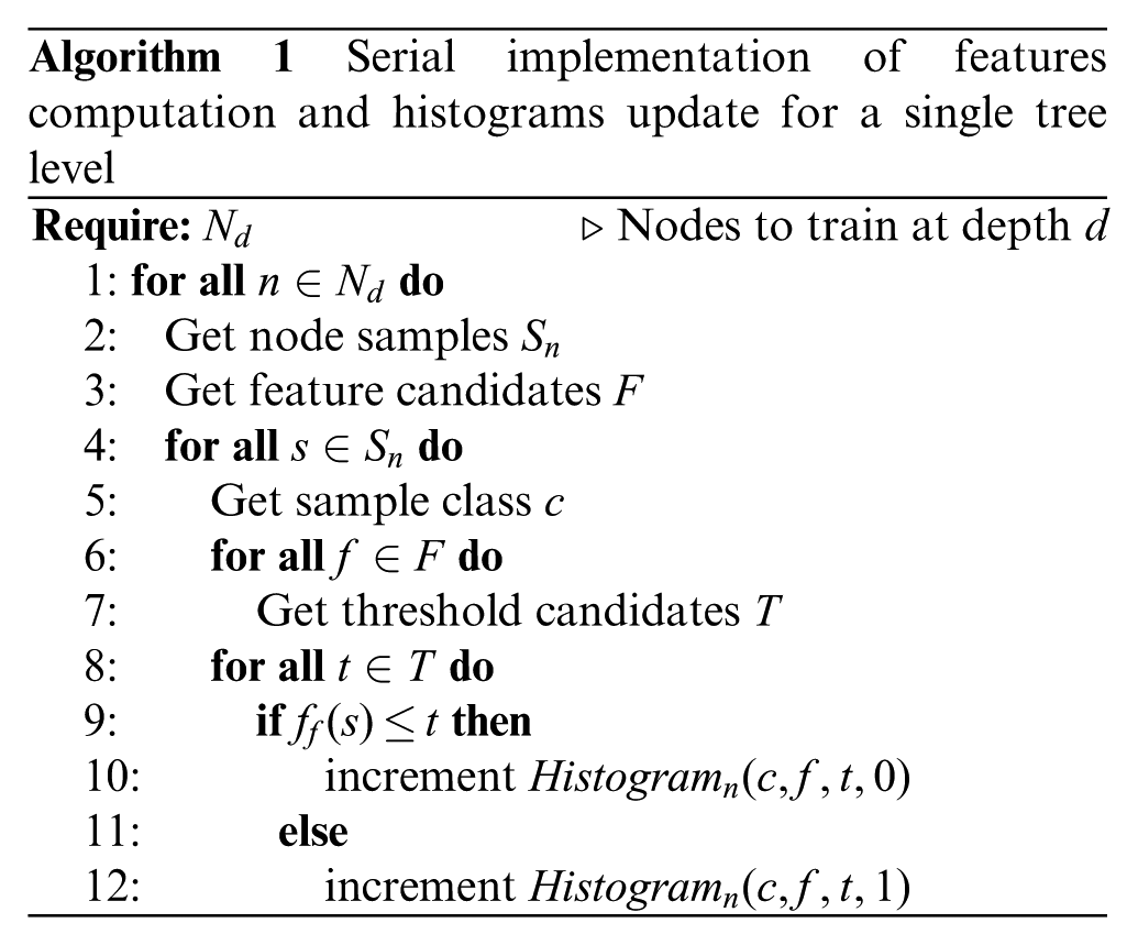
The cost of GPU-parallelized training must consider the time of image transfers since the limited capacity of GPU main memory is usually not sufficient to store the entire training set. The $HistogramUpdate$ term can thus be approximated as the following:

O_{HistUpdate} = O (\frac{I \times S \times F \times T}{α}) + \underset{ImageTransfers}{\underset{︸}{O (\min (\frac{S}{2^{d - 1}}, 1) \times I \times 2^{d - 1})}},

(9)

under the worst case assumption that image samples are perfectly split between left and right child for each node; α represents the speed-up factor of the GPU implementation, whereas ImageTransfers is the per-level cost of moving images to the GPU. As long as the fraction term $S / S 2^{d - 1} 2^{d - 1}$ is greater than 1, all training images must be transferred to the GPU for each node, and the transfer cost doubles at each level. Since features are computed on the fly, even if only a single pixel reaches the current node, the whole image must be loaded into the GPU main memory. Furthermore, images are transferred through the PCI bus; due to its limited bandwidth, this can easily represent the major bottleneck for the implementation if the GPU stays idle waiting for the images. At deeper levels, therefore, the ImageTransfers cost term dominates the per-level computational cost.

To reduce the number of image transfers, we introduce two new types of histograms: a local histogram L, which stores samples count for a single image, and a global histogram H, which instead aggregates samples count over all the nodes at the current level. More specifically, the local histogram is a 3D matrix of $S \times F \times T$ binary variables kept in the GPU memory in which a value of 1 means that, for the f-th/t-th feature/threshold pair, the s-th pixel has been forwarded to the left child, while a value of 0 means that the same pixel has been forwarded the right child. The global histogram is a four-dimensional matrix of $N \times C \times F \times T$ counters stored in the host RAM. It is equivalent to the histogram computed in Algorithm 1 but stores counters for all the nodes at the current level. Using the local and global histograms, we can rewrite the computation of features and histograms update loop over the training set images, as shown in Algorithm 2. Lines 2–9 update the local histogram for the current image and will be parallelized on the GPU, while lines 10–17 update the global histogram on the basis of the values of the local histogram bins. The complexity cost of the $HistUpdate$ term can now be approximated as follows:

O_{H i s t U p d a t e} = \underset{L o c a l U p d a t e}{\underset{︸}{O (\frac{I \times S \times F \times T}{α})}} + \underset{G l o b a l U p d a t e}{\underset{︸}{O (I \times S \times F \times T)}} + \underset{I m a g e T r a n s f e r}{\underset{︸}{O (I)}} + \underset{L o c a l H i s t R e a d}{\underset{︸}{O (S \times F \times T)}},

(10)

where the $LocalUpdate$ term refers to the cost of computing features and updating the local histogram on the GPU and the $GlobalUpdate$ term is the cost of global histogram update on the host. The remaining terms are associated with the cost of reading the local histogram $(LocalHistRead)$ from the GPU and moving images to the GPU $(ImageTransfer)$ . Rewriting the per-level training loop with respect to images leaves the amount of computation on sampled pixels unaltered while reducing the number of image transfers needed (every image needs to be moved only once for each trained level). We can avoid the additional cost of updating the global histogram and reading the local histogram by overlapping GPU/CPU computation and GPU execution with memory transfers as explained in Sections 3.3.1 and 3.3.2.

Algorithm 2

Algorithm 2 Features computation and local/global histograms update
Require: $T$ $▹$ Training set
1: for all $I \in T$ do
2: for all $s \in I$ do
3: Get reached node $n$
4: Get feature candidates $F$
5: for all $f \in F$ do
6: Get threshold candidates $T$
7: for all $t \in T$ do
8: if $f_{f} (s) \leq t$ then
9: increment $L (s, f, t)$
10: for all $s \in I$ do
11: Get reached node $n$
12: Get feature candidates $F$
13: Get current sample class $c$
14: for all $f \in F$ do
15: Get threshold candidates $T$
16: for all $t \in T$ do
17: $H (n, c, f, t) + = L (s, f, t)$

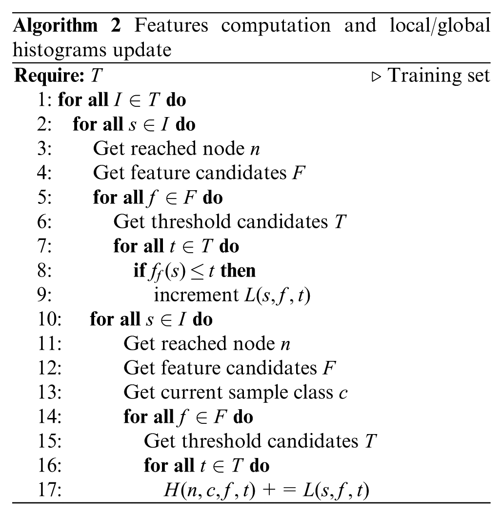
A possible limitation of this approach is that, since we iterate over images, processed pixels can reach an arbitrary number of nodes and the global histogram needs to count samples for all the leaf nodes at the currently trained level. Since the number of nodes doubles at each depth level, the global histogram size could reach the storage limitations of the host RAM when training the last levels of the tree. Nevertheless, in our experiments, the capacity of the host memory was usually sufficient to store the whole global histogram. Furthermore, due to the pruning resulting from termination criteria met at lower levels, the number of trained nodes tends to decrease in the last levels and so does the global histogram size.

Finally, instead of storing a counter in the global histogram for both left and right child, we keep a per-class counter of the total samples at node n and thus compute the right child counter for the f-th/t-th pair as the difference between the per-class counter and the histogram entry. Storing only the left counters allows us to halve the size of the global histogram, thereby drastically reducing its memory occupancy.

3.2. GPU implementation

The training main loop (Algorithm 3) iterates over tree levels up to the level specified by the $MaxDepth$ argument. The inputs are the training set images $TrainingSet$ , the current tree $Tree$ and the maximum depth $MaxDepth$ .

Algorithm 3

Algorithm 3 Training main loop
Require: $TrainingSet$
Require: $Tree$
Require: $MaxDepth$
1: for all $d \in 1 \dots MaxDepth - 1$ do
2: $ℱ, ℋ \leftarrow BOOTSTRAP (T r e e, d)$
3: for all $I \in TrainingSet$ do
4: $N \leftarrow PREDICT (ℐ, T r e e, d)$
5: $Θ_{ℐ}, T_{ℐ} \leftarrow SAMPLECANDIDATES (ℐ, N)$
6: $L \leftarrow COMPUTELOCALHISTOGRAM (ℐ, Θ_{ℐ}, T_{ℐ})$
7: $UPDATEGLOBALHISTOGRAM (L, ℐ, Θ_{ℐ}, T_{ℐ}, N, H)$
8: $Θ, T \leftarrow LEARNBESTFEATURESTHRESHOLDS (ℱ, H)$
9: for all $l \in F$ do
10: $UPDATENODE (l, Θ (l), T (l))$

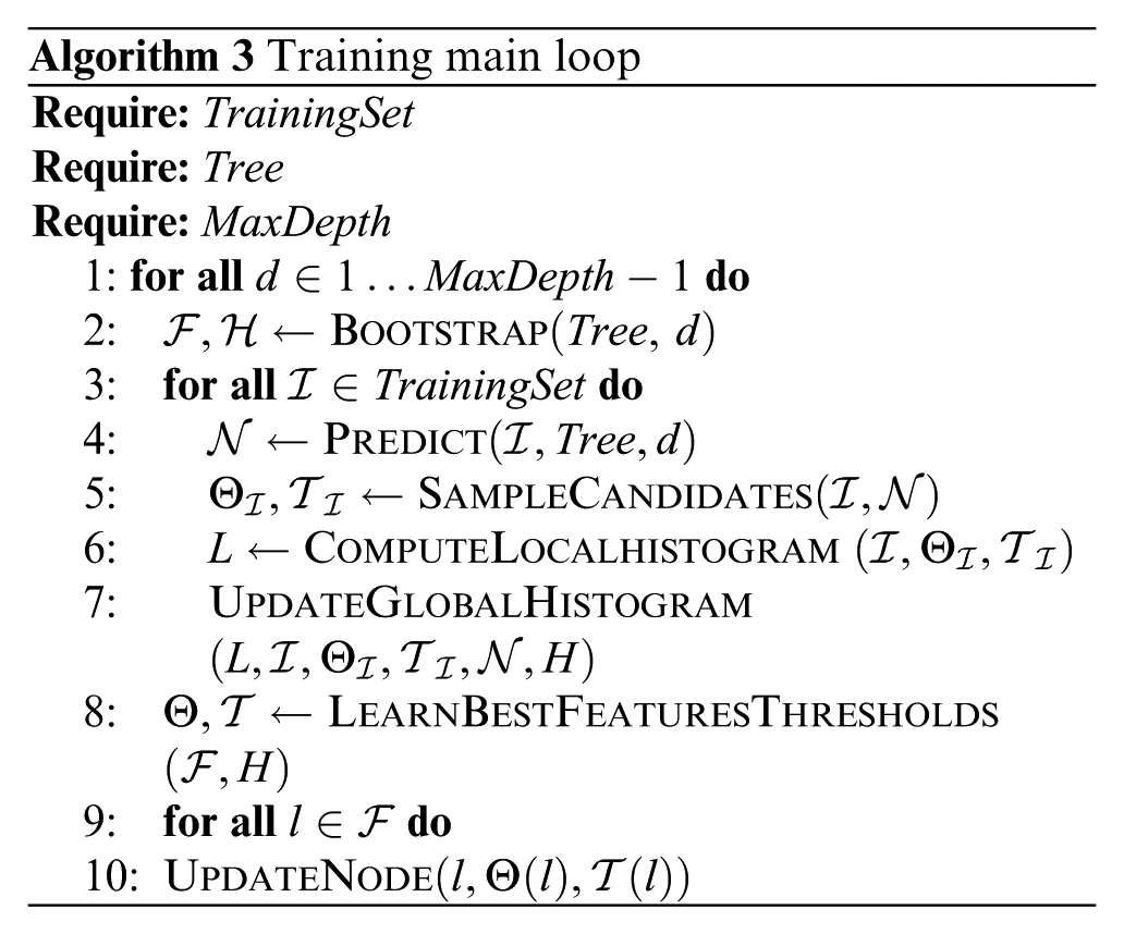
The first step performed for each level is to initialize the global histogram H and the frontier $F$ . $F$ stores the indexes of the nodes to train at the current level; it contains only the root node at depth 1 and the indexes of all the leaf nodes that still have not satisfied the stopping criteria at following levels.

The inner loop of lines 3–7 iterates over training set images $I$ . Each image stores one or more channels, the per-pixel class labels and a list of sampled pixels. The inner functions in lines 4–8 are responsible for the computation of histograms and best features/thresholds selection. They represent the core of the training phase and will be examined in detail in the following sections.

Finally, for each frontier node l, the UpdateNode function updates the node split function parameters and creates two new child nodes.

3.2.1. Leaf node prediction

To reduce the memory occupancy of the training set, we do not store the index of the leaf node currently reached by each image sample. Following the same approach of Sharp (2008), we instead perform a prediction step in kernel Predict. Given the current tree, we spawn $W \times H$ work items, one for each pixel, where W and H are the width and height of the current image, respectively; starting from the root node, each work item processes a single pixel as described in Section 2.1.1. The kernel outputs an image $N$ where, at each pixel, the index of the node reached at current depth d is stored.

3.2.2. Sampling of feature and threshold candidates

Starting from the second tree level, image samples span across multiple nodes. This can be problematic for the generation of feature and threshold candidates since, for each sample s that reaches a leaf node l, we need to access the sets of $Θ (l)$ feature vectors and $T (l)$ scalar thresholds sampled for that node. Furthermore, generating candidates at the beginning of each level for all the leaves is not feasible because that would easily saturate the memory as the training proceeds to deeper level.

For each image sample s, we generate feature and threshold candidates on the fly by means of a state-less pseudo-random number generator based on the MD5 cryptographic hashing function in the same fashion of Tzeng and Wei (2008). The use of the MD5 presents various advantages such as generation of high-quality random sequences and high throughput.

For each image, the SampleCandidates kernel launches $S \times F$ work items for S sampled image pixels and F per-node sampled features. Each work item initializes a four unsigned integers seed as $(t, n, f, 0)$ , where t, n and f are the indices of the current tree, the leaf node and the feature, respectively (the index n is obtained accessing the $N$ image computed by the Predict kernel). The seed is used as the input of the MD5 function, which outputs a vector of four unsigned integers. These values are normalized in the $[0, 1]$ range and used to draw a sample for each of the first four values of the feature vector. The process is repeated using the output values as next seed until all the feature vector entries are computed. Once the feature vectors have been sampled, the process is repeated for the threshold candidates, substituting the fourth initial seed entry with 1. The function returns a set of $S \times F$ feature vectors $Θ_{I}$ and a set of $S \times F \times T$ per-feature scalar thresholds $T_{I}$ .

While in Algorithm 3 the candidates sampling has been kept separated by the local histogram computation, they are actually implemented in the same OpenCL kernel. This allows to keep feature and threshold candidates in GPU registers, thus avoiding access to the global main memory.

3.2.3. Local histogram computation

The ComputeLocalHistogram kernel computes the feature responses for the current image samples and updates the local histogram accordingly. We launch $S \times F$ work items, each of which computes the $f_{Θ_{I} (s, f)} (s)$ feature response, where s and f are the current sample and feature indices and s represents the pixel coordinates of the sample. The feature response is then compared with each entry of the threshold candidates $T_{I} (s, f, t)$ and the corresponding local histogram bin $(s, t, f)$ is set to 1 if the sample is forwarded to the left child $(f_{Θ_{I} (s, f)} (s) \leq T_{I} (s, f, t))$ . Each work item works on a different histogram bin, so no synchronization is needed.

Since work items are scheduled with respect to the last dimension of their local ID, indexing the local histogram with respect to the feature at the last dimension allows consecutive work items to access adjacent bins, allowing coalescing and reducing the number of memory transactions for local histogram update.

3.2.4. Global histogram update

The UpdateGlobalHistogram function updates the global histogram H accordingly to the local histogram L entries. Due to its larger size, H is kept in host memory (i.e. computer RAM) and thus the function is executed by the host. We iterate over local histogram bins and, for each bin $L (s, t, f)$ , we increment the corresponding bin $H (n, c, t, f)$ if the local histogram bin has been set to 1. The index n and the class c are obtained by accessing the leaf node indices image $N$ computed by the Predict kernel and the training set image $I$ . After all the local histograms have been processed, H stores the total number of samples that follow the left branch of the frontier nodes $F$ for each tuple $(c, t, f)$ . As in the case of local histogram, the last dimension of the global histogram is associated with the feature index, allowing looping on consecutive bins for both histogram types and thus maximizing cache coherency. To further improve performances, global histogram bins are incremented concurrently using SSE2 instructions.

At deeper levels, due to the increasing number of leaf nodes, the size of the global histogram could reach the memory limits of the host. In this case, we split H into multiple histograms, one for each frontier subset, and we repeat the inner loop of Algorithm 3 multiple times, working only on the image samples that reach the leaves in the current subset.

3.2.5. Best feature/threshold pairs calculation

The aim of this phase is to compute the information gain of a leaf node l for each feature/threshold pair using the global histogram counters. For each node at the current depth, we spawn multiple work items and assign to each one a subset $(F \times T \times C) / (F \times T \times C) p p$ of the total histogram bins for the current leaf node l, with p the number of pairs $(f, t)$ processed by the current work item. At deeper levels, multiple nodes can be processed in parallel.

After the information gain has been computed for all the pairs, the indices of the best feature/threshold combination are returned to the host and used to update the node parameters (i.e. the feature vector θ and the threshold τ).

3.3. GPU optimizations

Feature and image types support

Instead of hard-coding the feature computation routine, we provide to the users an entry point to define arbitrary per-pixel features. We export a ComputeFeature OpenCL function prototype whose implementation code must be provided by the user through a feature.cl file. The function will be called by both the Predict and ComputeLocalHistogram kernels to calculate the feature response at each pixel of the processed image.

We further generalize our implementation with respect to image types, supporting arbitrary pixel format and number of channels. More specifically, we map images up to four channels to single-channel OpenCL image objects, with format CL_R, CL_RG, CL_RGB or CL_RGBA, depending on the number of channels. If the training images have more than four channels, we map them to single-channel OpenCL 3D images, where the number of 2D slices corresponds to the original number of channels.

3.3.1. Overlap of local and global histograms computation

Although local and global histogram processing is executed sequentially for a single image, we can overlap the global histogram update of the current image with the local histogram computation of the next image in the training loop. This is shown in Figure 4.

We launch two host threads: one responsible for data transfers to/from the GPU and for kernel launching and the other reserved for global histogram update. The two threads communicate through a FIFO queue. Once a pair of node indices image $N$ and local histogram L have been computed by the GPU, they are pushed into the queue by the first thread and made available to the second thread. The former can continue with the processing of the next image, while the latter updates (in parallel) the global histogram. The two phases are thus completely overlapped and the total execution time is given from the slowest one. Supposing that the cost of prediction, sampling of candidates and nodes image reading is negligible, the cost of histograms update can thus be reduced to the following:

O_{HistUpdate} = \max (O_{ImageTransfer} + O_{LocalUpdate} + O_{LocalHistRead}, O_{GlobalUpdate}) .

(11)

3.3.2. Overlap of local histograms transfer and computation

Current generations of GPU devices are capable of concurrent data transfer to/from the GPU and kernels execution. We can leverage this feature to overlap the computation of the local histogram for the current image with the reading of the one calculated on the previous image. Since local histogram size is linear with respect to the number of sampled pixels, features and thresholds, when their number increases the time spent reading the histogram from the GPU becomes significant. The overlap of local histogram reading and computation is shown in Figure 5. We initialize two command queues and, at each iteration, one queue writes the image to GPU memory and launches the local histogram computation kernel, while the other reads the local histogram previously computed. On the next iteration, the role of the two queues is swapped. In our experiments, the kernel execution time is commonly greater than the reading time, so we can manage to mask the local histogram transfer time (LocalHistRead term of equation (9)) and consequently reduce the image processing time, obtaining a final cost of histograms update as in the following equation:

O_{HistUpdate} = \max (O_{ImageTransfer} + O_{LocalUpdate}, O_{GlobalUpdate}) .

(12)

4. Experimental results

We compare our implementation with the library CUDA Random Forest For Image Labeling (CURFIL) described in Schulz et al. (2015). At the time of writing, this is in fact the only available RF implementation applicable to CV applications which uses the local features of Section 2.2 and which is accelerated using GPUs. The comparison is carried out on two publicly available datasets: the MSRC2 data set (Microsoft Research, 2015) and the NYU2 data set (Silberman et al., 2012).

We train multiple RF trees sequentially and measure the average per-tree training time with respect to an increasing number of sampled pixels per image and sampled features per node. We also provide classification accuracy results when available since the CURFIL library is not able to perform prediction with dense trees (tree size is limited to 32,768 nodes). This usually happens when more samples are extracted from images and, thus, the stopping criteria for nodes are met at lower levels.

Finally, we test the performance of our implementation with large training sets using a data set of about 100 K images, which represent the static signs of the Italian Sign Language (LIS).

We perform our experiments on an Intel Core i7-3770 machine, paired with 32 GB of RAM and a Nvidia GeForce 670 GPU (2 GB of DDR5 RAM). We limit the memory reserved for global histogram allocation to 24 GB.

4.1. MSRC2 data set

The MSRC2 data set contains a total of 591 (256 for training, 256 for testing and 79 for validation) labelled colour images belonging to 23 classes. As in Schulz et al. (2015), we train on the training plus validation set using the feature of equation (6), and we treat the classes horse and mountains as background. We also use the same feature parameters suggested by the authors (offset 95 px, region size 12 px, 20 thresholds, stop criteria of 38 minimum pixels per node), except for the threshold sampling (random sampling of feature responses for CURFIL, uniform sampling in the range [−152, 152] in our implementation), and the number and maximum depth of the trees, which are fixed at 5 and 20, respectively.

The results for the MSRC2 data set are reported in Table 1. We manage to reduce the training time of our implementation with respect to the CURFIL library by a factor between 1.35 and 2.02. For both implementations, the average training time increases almost linearly with respect to the number of sampled pixels and features. Figure 6(a) and (b) shows the per-level training time for 512 sampled pixels and 1024 sampled features. In this case, we achieve the maximum speed-up of 2.02. For our implementation, the first half of the depth levels are trained in nearly constant time. Furthermore, we manage to achieve a full overlap of the global and local histogram computations. We can also notice that at initial depths the per-level training time is almost equivalent for the two libraries. As the depth increases and the number of leaf nodes doubles, the impact of histogram aggregation needed for best features/thresholds calculation becomes noticeable and the per-level training time increases, especially for the CURFIL library. Our implementation performs histogram aggregation in less time and thus reduces the total training time with respect to the CURFIL library.

Table 1.

Average per-tree training time (in seconds) on the MSRC2 data set for different values of sampled pixels and features.^a

Samples	Features
Samples	512	1024	2048	4096
512	35.35	66.14	125.14	237.45
	21.69	32.80	65.77	122.17
	(1.63X)	(2.02X)	(1.90X)	(1.94X)
1024	63.66	115.88	225.77	415.52
	36.75	60.24	123.18	234.17
	(1.73X)	(1.92X)	(1.83X)	(1.77X)
2048	108.24	198.74	383.50	722.71
	66.77	113.48	230.68	446.04
	(1.62X)	(1.75X)	(1.66X)	(1.62X)
4096	179.01	334.45	668.18	1230.33
	122.74	213.34	429.07	909.33
	(1.46X)	(1.57X)	(1.56X)	(1.35X)

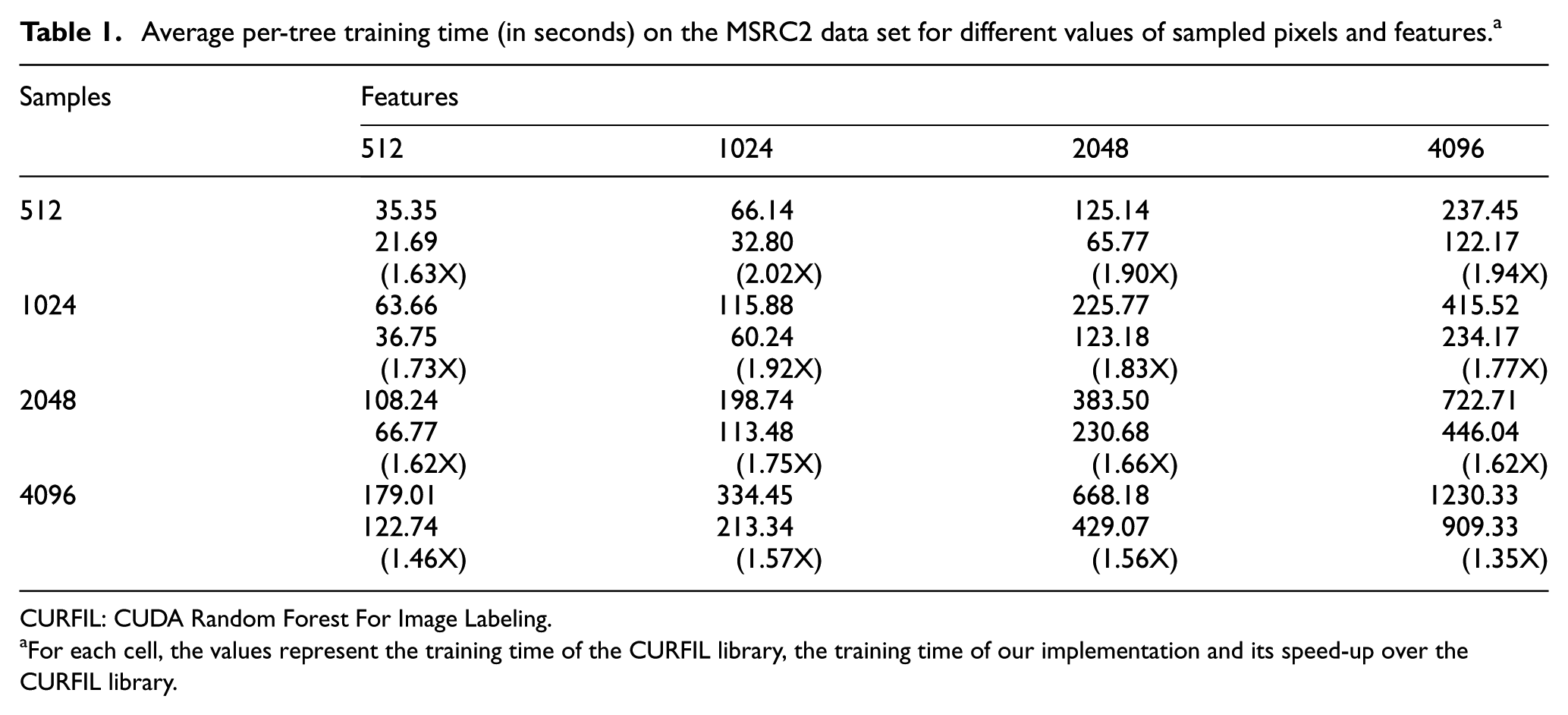
CURFIL: CUDA Random Forest For Image Labeling.

For each cell, the values represent the training time of the CURFIL library, the training time of our implementation and its speed-up over the CURFIL library.

For 4096 sampled pixels and 4096 features, the gain in total training time of our implementation over CURFIL decreases, as shown in Figure 6(c) and (d). For this combination of sampled pixels and features, we achieve the minimum speed-up factor of 1.35. Due to the increasing number of pixels and features, more time is spent on features computation and the impact of histograms aggregation is reduced.

It should be noted that the MSRC2 data set represents a favourable context for the CURFIL library. Due to the limited dimension of the training set, the whole set of images resides on the GPU and only an initial transfer is required during the training.

Table 2 reports the average per-pixel and per-class classification accuracy. For 512, 1024 and 2048 sampled pixels, we have values for both libraries, with a minimum average gain of 0.09% in per-pixel accuracy and a limited average loss of 0.12% in per-class accuracy over the CURFIL library. The classification accuracy for the two implementations can therefore be considered equivalent.

Table 2.

Per-class and per-pixel accuracy on the MSRC2 data set for different combinations of sampled pixels and features.^a

Samples	Features
Samples	512	1024	2048	4096
512	49.84, 36.05	50.22, 36.70	51.12, 37.38	51.55, 38.03
512	49.35, 35.25	50.54, 36.64	51.00, 37.00	51.61, 37.60
1024	49.86, 36.55	51.06, 37.58	51.89, 38.45	52.43, 39.07
1024	50.13, 36.44	51.45, 37.99	51.70, 38.18	52.63, 38.98
2048	( \ )	51.53, 38.53	52.25, 38.97	52.39, 39.32
2048	50.70, 37.44	51.64, 38.44	52.23, 38.98	52.85, 39.74
4096	( \ )	( \ )	( \ )	( \ )
4096	50.89, 37.70	51.72, 38.70	52.34, 39.29	53.16, 40.12

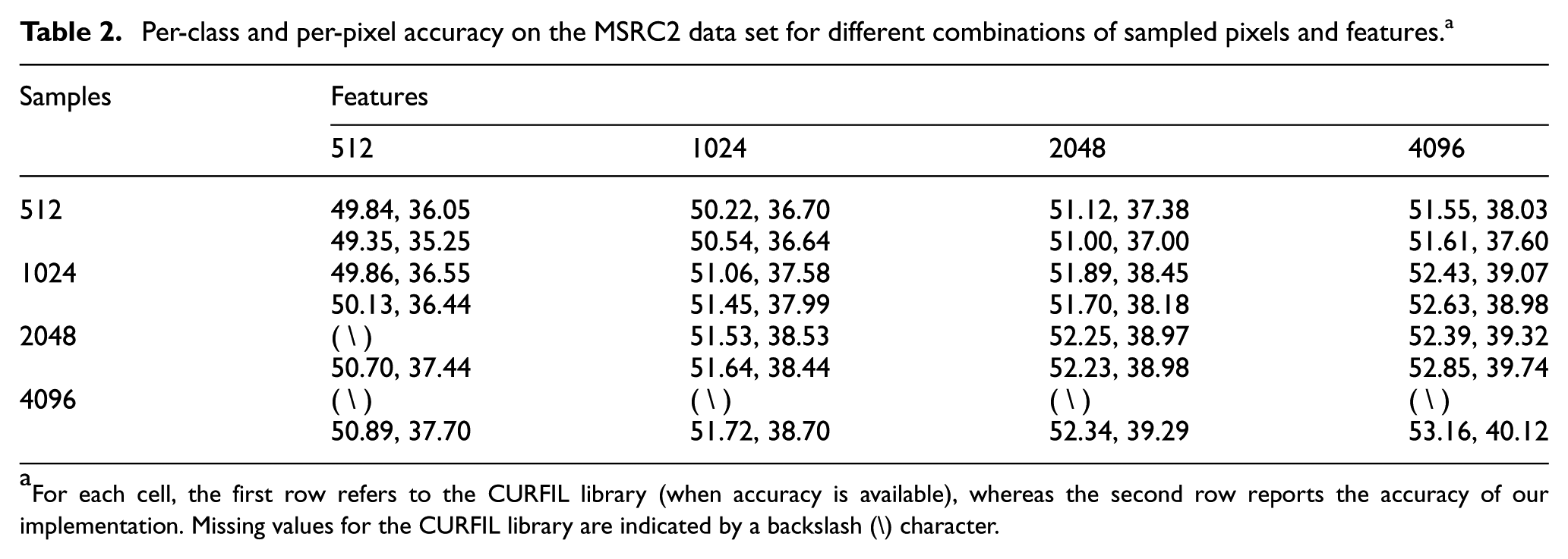
For each cell, the first row refers to the CURFIL library (when accuracy is available), whereas the second row reports the accuracy of our implementation. Missing values for the CURFIL library are indicated by a backslash (\) character.

4.2. NYU2 data set

The NYU2 data set contains 1449 densely labelled RGB-D images acquired from a variety of indoor scenes using a Kinect sensor. We use the same train/test split suggested in Schulz et al. (2015), resulting in a training set of 795 images and 654 images left out for testing. Labelling distinguishes between four semantic classes: ground, furniture, structure and props. Since depth information is also available, we use the RGB-D features defined in Stuckler et al. (2012). As for the previous data set, we use the training parameters suggested in Schulz et al. (2015) (offset 111px, region size 3px, 20 thresholds, stop criteria of 204px, 3 trees trained up to depth 18). We fix the thresholds sampling range to [−267, 267]. Unlike the MSRC2 data set, the main memory capacity of the GPU of our configuration is not sufficient to store all training images.

Table 3 reports the training times for the NYU2 data set: we obtain a speed-up factor variable between 2.39 and 18.93. With an increasing number of images with respect to the MSRC2 data set, more samples reach the lower levels of the trees. This translates to a greater number of image transfers to the GPU as predicted by the ImageTransfers term of equation (9). The CURFIL library implements some overlap of image transfers and features calculation, but the computational load is not sufficient to mask the transfer cost. As a result, the per-level training time is bound by the time of image transfers since the initial levels, as shown in Figure 7(b) for 4096 samples and 512 features. For this combination of sampled pixels and features, we achieve a speed-up factor of 18.93 with respect to the CURFIL library (Figure 7(a)).

Table 3.

Average per-tree training time (in seconds) for the NYU2 data set.^a

Samples	Features
Samples	512	1024	2048	4096
512	499.32	517.23	533.00	558.88
	64.04	84.94	137.10	233.89
	(7.80X)	(6.09X)	(3.89X)	(2.39X)
1024	1026.42	1050.54	1117.43	1156.49
	85.57	127.35	230.70	423.56
	(11.99X)	(8.25X)	(4.84X)	(2.73X)
2048	2047.57	2104.70	2158.49	2304.40
	127.43	214.64	416.00	800.57
	(16.07X)	(9.81X)	(5.19X)	(2.88X)
4096	4102.00	4139.39	4364.27	4616.66
	216.66	388.68	781.34	1562.95
	(18.93X)	(10.65X)	(5.59X)	(2.95X)

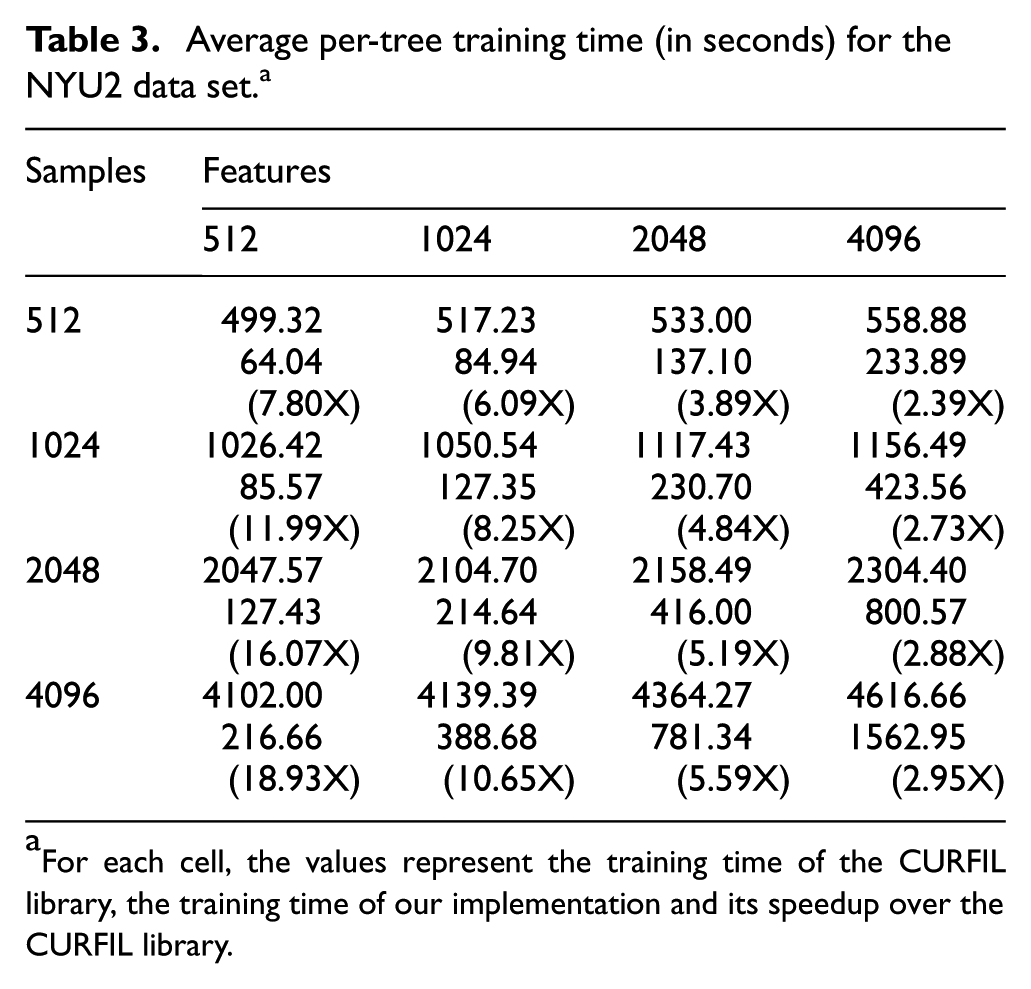
For each cell, the values represent the training time of the CURFIL library, the training time of our implementation and its speedup over the CURFIL library.

For increasing number of sampled features, the growth of the total training time for the CURFIL library is minimal. This is shown in Figure 7(d). If we keep 4096 sampled pixels and increase the number of features from 512 to 4096, even if the workload increases (as noticeable for the first levels), starting from depth 5 the cost of features computation and histograms update is completely outweighed by the cost of moving images to the GPU. Once again, this confirms that the training time is bound by the time of image transfers. For our implementation, training time increases with a larger number of sampled features, thus reducing the speedup factor with respect to the CURFIL library. Nevertheless, even for 4096 features, we obtain a speed-up factor of 2.95 (Figure 7(c)). As in the case of the MSRC2 data set, we also manage to completely overlap the global and local histograms computation. Furthermore, due to the increased training set size, more time is spent processing images and the impact of histogram reduction is minimal. We therefore obtain a nearly constant training time for all depth levels.

Table 4 reports the classification accuracy of both implementations. The performances are comparable, with a slight average drop in per-pixel and per-class accuracy for our implementation of 0.34% and 0.42%, respectively. We ascribe the accuracy loss to the different sampling strategy for the feature thresholds since it represents the major difference in the training procedure of the two libraries. To confirm our hypothesis, we modified the CURFIL library and replaced the original threshold sampling strategy (sampling of feature responses over sampled pixels) with a random sampling within the predefined range [−267, 267]. This modification degrades the classification performance of the CURFIL library and yields an average drop in per-pixel and per-class accuracy with respect to our implementation of 0.11% and 0.15%, respectively, making the accuracy of the two approaches equivalent.

Table 4.

Per-pixel and per-class accuracy for the NYU2 data set.^a

Samples	Features
Samples	512	1024	2048	4096
512	66.96, 63.42	67.09, 63.64	67.18, 63.92	67.31, 64.03
512	66.68, 62.83	66.79, 63.09	67.05, 63.52	67.17, 63.71
1024	67.33, 63.86	67.68, 64.34	67.69, 64.49	67.69, 64.62
1024	66.96, 63.32	67.20, 63.70	67.38, 64.08	67.64, 64.34
2048	67.77, 64.39	67.88, 64.67	67.96, 64.80	68.21, 65.10
2048	67.19, 63.80	67.46, 64.21	67.72, 64.56	67.85, 64.77
4096	67.93, 64.64	68.13, 64.88	68.26, 65.17	68.46, 65.46
4096	67.38, 64.19	67.62, 64.56	67.89, 64.91	68.06, 65.15

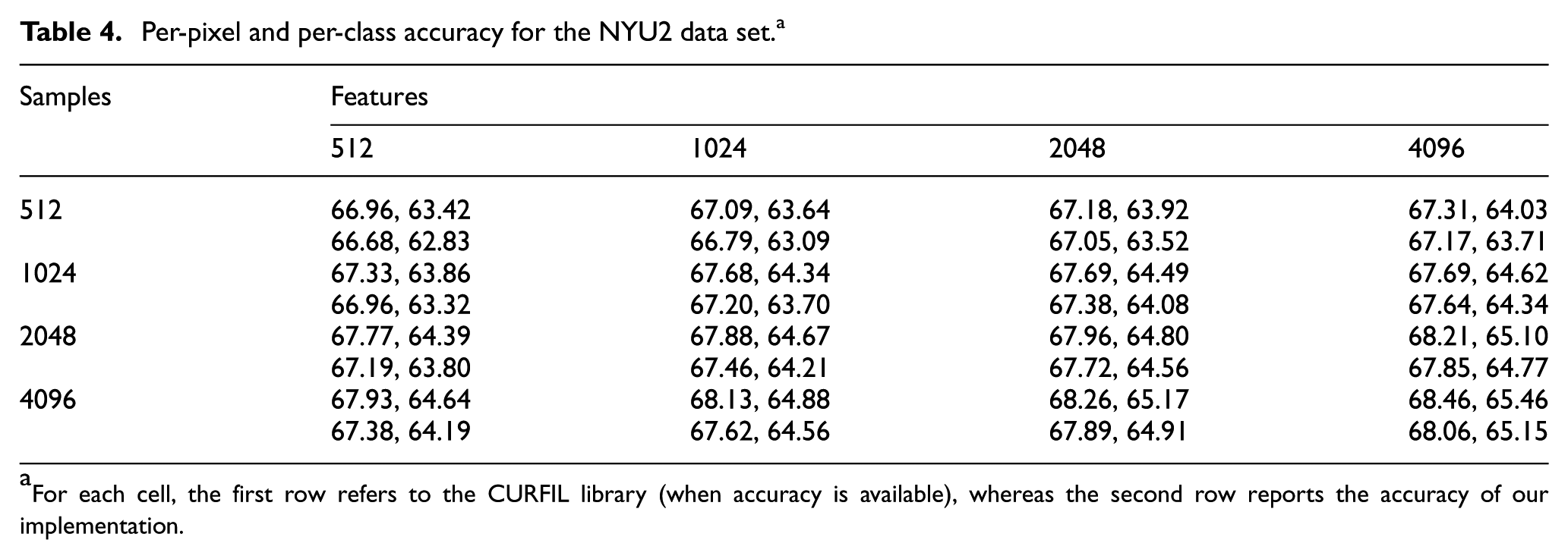
For each cell, the first row refers to the CURFIL library (when accuracy is available), whereas the second row reports the accuracy of our implementation.

The limited accuracy drop has a negligible impact on the classifier performance, and it is largely outweighed by the substantial reduction in training time. Furthermore, according to the state of the art CV applications of RF that use local features, the random number of samples for both image pixels and node features is usually limited to around 2 K samples (e.g. Kazemi et al., 2014; Keskin et al., 2011; Shotton et al., 2011). Increasing these values yields a marginal accuracy gain that is largely outweighed by the increase of the training times. Using a combination of 1024 or 2048 samples for pixels and features we keep an accuracy close to the best one (0.36% and 0.44% lower for per-pixel and per-class accuracy, respectively) and still manage to obtain a speedup factor between 4.84 and 9.81.

4.3. LIS data set

The LIS data set contains 100 K labelled depthmaps representing the static signs associated with alphabet letters and digits. The depthmaps are synthetically generated by means of 3D rendering in the same fashion of Russo et al. (2015). Different hand parts (e.g. fingertips, palm, wrist, etc.) are labelled with different colours for a total of 22 unique labels, as shown in Figure 8. The data set contains also 83 manually labelled depthmaps acquired from an LIS signer by a Kinect sensor and used for testing. We used the depth-only features of equation (7) and chose the following training parameters: 2048 sampled pixels, 2048 sampled features, 60px offsets, 20 thresholds sampled in the range [−200, 200] and 3 trees trained up to depth 20.

Figure 9 shows the per-level training time for the LIS data set. For levels up to the 13-th, we manage to keep the training time constant. Compared to the MSRC and the NYU2 data set, the global histogram update represents the most time-consuming part. This is due to the lighter computational weight of the depth-only features with respect to the ones based on image regions we applied to the previous data sets.

Due to the larger size of the training set, more pixel samples reach the lower levels of the trees and the pruning caused by the stopping criteria on the minimum number of samples is less frequent. Since the global histogram size is linear with respect to the number of nodes in the current level, its dimension doubles at each level. At deeper levels (from level 14 onward), the host memory allocated is not sufficient to store the global histogram entirely and we need to split it in multiple slices, as explained in Section 3.2.4. For each image, sampled pixels are processed only if they reach a node in the current slice. This allows us to limit the increase of global histogram time update, as shown for the last levels in Figure 9. Since less processing is also performed by the GPU for the features computation and local histogram update, we are not able to mask the local histogram transfer time, with a corresponding increase of the per-level total time associated to local histogram computation. We have different options to tackle this problem: we can reduce the global histogram size by reducing the number of sampled pixels/features/thresholds (at the expense of a partial accuracy loss) or we can increase the threshold on minimum pixel per node to make the pruning more frequent. Despite the increase of training time that affects the last levels, we still manage to train a single tree in less than 23 hours. For comparison, in Budiu and Shotton (2011), training a similar data set (body parts instead of hand parts) with the same parameters (except for the number of thresholds that is raised from 20 to 50) and 300 K images per-tree takes around 1 day on a cluster of 1000 CPUs. Our implementation is thus able to handle data sets of comparable size and keep the same order of magnitude in terms of training time using consumer-grade GPUs.

Finally, we obtain a per-pixel accuracy of 64.16% and a per-class accuracy of 58.94%. These results are comparable to Keskin et al. (2011).

5. Conclusions and future work

We presented a novel approach to train RF on GPU for CV applications using simple per-pixel local features. We trained the classifier in a breadth-first fashion and parallelized the training with a per-image granularity, allowing reduction in the number of required image transfers and the overhead of data transfers to/from the GPU when the data set cannot be entirely stored in GPU main memory. Furthermore, our implementation has some additional distinctive features, like on-the-fly generation of random feature/threshold candidates using a hash function, support for arbitrary image types and the possibility for the user to specify custom features. We compared our implementation with the state of the art on the MSRC2 and NYU2 data set. Our RF performs comparably in terms of classification accuracy for both data sets, while reducing training time up to 1.6 times for the MSRC2 data set and between 2 and 18 times for the more challenging NYU2 data set. We also tested our implementation with a large data set of around 100 K images and managed to train a single tree in less than 1 day, demonstrating how our approach trains big data sets in reasonable time using consumer-grade GPU devices.

Finally, we released the source code of our RF implementation publicly, allowing more researchers to further experiment with different data sets and feature types while drastically reducing training times.

Footnotes

Declaration of Conflicting Interests

The author(s) declared no potential conflicts of interest with respect to the research, authorship, and/or publication of this article.

Funding

The author(s) disclosed receipt of the following financial support for the research, authorship, and/or publication of this article: This work was supported by the Italian Ministry of Health, Ricerca Finalizzata 2009 - VRehab Project (Grant RF-2009-1472190).

1.

An OpenCL-accelerated Random Forests implementation for Computer Vision applications using local features. Available at: (accessed 1 November 2015).

Author biographies

Daniele Pianu received the MSc degree in Computer Engineering from the Politecnico di Torino in 2013. He is a research fellow in the Engineering for Health and Wellbeing Group at the Institute of Electronics, Computer and Telecommunication Engineering (IEIIT) of the National Research Council (CNR) of Italy. His current research fields include computer vision, human-computer interfaces development and high-perfomance computing on GPU.

Roberto Nerino received the degree in Electronic Engineering and the PhD in Metrology from the Politecnico di Torino in 1982 and 1994, respectively. From 1989 to 2007 he was a researcher of the National Institute of Metrological Research (INRIM), and in 2007 he joined the Institute of Electronics, Computer and Telecommunication Engineering (IEIIT) of the National Research Council (CNR) of Italy. He has been coordinator of several research projects funded by industries and research institutions and a promoter of collaborations with European universities. He is co-author of 4 patents and over 60 papers in refereed journals and conferences. His research interests include image processing, human-computer interaction, computer vision techniques and body sensor networks for motion analysis and body tracking in healthcare monitoring and rehabilitation applications.

Claudia Ferraris received the degree in Information Science (summa cum laudae) from the University of Turin, Italy, in 1997. In 1998 and 1999 she worked as researcher at the CSTV and IRITI institutes of the National Research Council (CNR) of Italy, respectively, with focus on image and video coding and motion estimation algorithms for H263 video coding standard. Since 2012 she is a research fellow at the Institute of Electronics, Computer and Telecommunication Engineering (IEIIT) of the CNR. Her current activity focuses on the development of tele-monitoring and tele-rehabilitation systems and human-computer interfaces for subjects affected by neurological disease and elderly subjects.

Antonio Chimienti graduated in Information Science (summa cum laudae) from the University of Turin, Italy, in 1987. Since 1988 he is with the Institute of Electronics, Computer and Telecommunication Engineering (IEIIT) of the National Research Council (CNR) of Italy where he is currently Senior Researcher. His former research activity was in video coding area in which he developed algorithms for vector quantization, wavelet coding, motion compensation, error resilience and error concealment. In 2002 he joined the Artificial Vision group of the IEIIT, where he worked on image processing and image understanding for application in the cultural heritage field, with focus on computer vision and non-contact metrology. More recently his interest moved to the real-time tracking of the human body by means of 3D cameras with applications in the medical field for remote rehabilitation and monitoring purposes.

References

Bradski

Kaehler

(2008) Learning OpenCV: Computer Vision with the OpenCV Library. Sebastopol, CA: O’Reilly Media, Inc.

Breiman

(2001) Random forests. Machine Learning45(1): 5–32.

Budiu

Shotton

(2011) Parallelizing the training of the Kinect body parts labeling algorithm. In: Big learning: Algorithms, Systems and Tools for Learning at Scale, Sierra Nevada, Spain, September, 2011, pp. 1–6.

Criminisi

Shotton

Konukoglu

(2012) Decision Forests: A Unified Framework for Classification, Regression, Density Estimation, Manifold Learning and Semi-supervised Learning. Boston: Now.

Grahn

Lavesson

Lapajne

. (2011) CudaRF: A CUDA-based implementation of random forests. In: IEEE/ACS International Conference on Computer Systems and Applications, Sharm El-Sheikh, Egypt, December 2011, pp. 95–101. Piscataway, NJ: IEEE.

Jansson

Bostr

(2014) gpuRF and gpuERT: efficient and scalable GPU algorithms for decision tree ensembles. In: IEEE International Parallel & Distributed Processing Symposium Workshops, Phoenix, AZ, 19–23 May 2014, pp. 1612–1621. Piscataway, NJ: IEEE.

Kazemi

Keskin

Taylor

. (2014) Real-time face reconstruction from a single depth image. In: 2nd International Conference on 3D Vision, Tokyo, Japan, 8–11 December 2014, pp. 369–376. Piscataway, NJ: IEEE.

Keskin

Kirac

Kara

. (2011) Real time hand pose estimation using depth sensors. In: IEEE International Conference on Computer Vision Workshops, Barcelona, Spain, 6–13 November 2011, pp. 1228–1234. Piscataway, NJ: IEEE.

Khronos Group (2015) OpenCL—the open standard for parallel programming of heterogeneous systems. Available at: https://www.khronos.org/opencl (accessed 8 July 2015).

10.

Liaw

Wiener

(2002) Classification and regression by randomforest. R News2(3): 18–22.

11.

Microsoft Research (2015) Image understanding. Available at: http://research.microsoft.com/en-us/projects/objectclassrecognition (accessed 8 July 2015).

12.

Munshi

Gaster

Mattson

. (2011, July) OpenCL Programming Guide. Boston: Pearson Education.

13.

NVIDIA Corporation (2015) About CUDA. Available at: https://developer.nvidia.com/about-cuda (accessed 8 July 2015).

14.

Pedregosa

Varoquaux

Gramfort

. (2011) Scikit-learn: machine learning in Python. Journal of Machine Learning Research12: 2825–2830.

15.

Russo

Airò Farulla

Pianu

. (2015) PARLOMA-a novel human-robot interaction system for deaf-blind remote communication. International Journal Of Advanced Robotic Systems12: 57.

16.

Schroff

Criminisi

Zisserman

(2008) Object Class Segmentation using Random Forests. In: British Machine Vision Conference, Leeds, UK, 1—4 September 2008, pp. 1–8.

17.

Schulz

Waldvogel

Sheikh

. (2015) CURFIL: Random Forests for Image Labeling on GPU. In: 10th International Conference on Computer Vision Theory and Applications, Berlin, Germany, 11—14 March 2015, pp. 156–164.

18.

Sharp

Implementing decision trees and forests on a GPU. In: Forsyth

Torr

Zisserman

(eds) 10th European Conference on Computer Vision, Marseille, France, 12–18 October 2008, pp. 595–608. Berlin Heidelberg: Springer.

19.

Shotton

Fitzgibbon

Cook

. (2011) Real-time human pose recognition in parts from single depth images. In: IEEE Conference on Computer Vision and Pattern Recognition, Colorado Springs, CO, 20—25 June 2011, pp. 1297–1304. Piscataway, NJ: IEEE.

20.

Silberman

Hoiem

Kohli

. (2012) Indoor segmentation and support inference from RGBD Images. In: 12th European Conference on Computer Vision, Florence, Italy, 7—13 October 2012, pp. 746–760. Heidelberg: Springer.

21.

Stuckler

Biresev

Behnke

(2012) Semantic mapping using object-class segmentation of RGB-D images. In: IEEE/RSJ International Conference on Intelligent Robots and Systems, Vilamoura, Portugal, 7—12 October2012, pp. 3005–3010. Piscataway, NJ: IEEE.

22.

Tzeng

Wei

(2008) Parallel white noise generation on a GPU via cryptographic hash. In:Symposium on Interactive 3D graphics and games, New York, NY, 15—17 February 2008, p. 79. New York: ACM.

23.

Waldvogel

(2013) Accelerating random forests on CPUs and GPUs for object-class image segmentation. Master’s thesis, Universität Bonn, Germany.