






Abstract
A fast, highly parallelized, simulation of unidirectional ultrasonic pulse propagating in a two-dimensional environment is presented. The pulse intensity versus time is recorded using an array of unidirectional ultrasonic receivers located at known locations and arranged in a small circle around the transmitter. To speed up the simulation process, OpenCL 2.0 heterogeneous compute language on a graphics processing unit is used. The simulation result is then compared with experimental data to validate its accuracy. By comparing both simulated and experimental data, the collected intensity–time profiles can be used to map an environment. Environments can be mapped using not only direct reflections but also higher order reflections from objects that are not directly seen by the transmitter. With the help of this simulation, subtle characteristics in an environment, such as a slight tilt or curvature, can be measured. The front end of the simulation is written using C#, while the back end is written using C\C++ and OpenCL.
1. Introduction
Using ultrasonic waves for imaging and nondestructive testing is an old and effective technique (Blitz and Simpson, 1995). Simulating ultrasonic waves enhances its application development processes. The currently published simulations target different applications. For example, Connolly (2009) used ray-tracing to model welds using FORTRAN. Many researchers used ultrasound simulations of medical images. For example, Burger et al. (2013) did an ultrasound simulation to synthesize realistic looking ultrasound images using GPU, and Mattausch and Goksel (2016) introduced a Monte Carlo ray-tracing technique to simulate realistic images. Rubi et al. (2017) implemented and compared two simulation models for training, and Tobias et al. (2009) used CUDA to simulate medical images. Multiple other authors used GPU-based ultrasound simulations (Haigh and McCreath, 2014; Jaros et al., 2012; Varray et al., 2011; Aguilar et al., 2013). Emmanuel et al. (2002) simulated ultrasonic waves based on finite-difference time-domain computations of the elastodynamic equations. Treeby et al. (2012) made a model based on coupled first-order acoustic equations valid for nonlinear wave propagation in heterogeneous media with power law absorption. He (1998) proposed a method to simulate the propagation of a broadband ultrasound pulse in a lossy medium whose attenuation exhibits a power law frequency dependence. Ultrasound simulations are usually developed with a specific application in mind. Developed simulations ranged from crack growth studies (Shen and Cesnik, 2017) to stress (Zhan et al., 2017), fatigue (Radecki et al., 2018), and damage in materials (Liu et al., 2016), to tissues characterization (Goncharsky et al., 2016).
In this work, a simulation of the propagation of directed ultrasonic pulses that have known intensity profiles in a two-dimensional (2-D) environment, with various detectors in known locations, is presented. The detectors listen for waves incoming from multiple specific directions and record analog intensity as a function of time, using OpenCL 2.0 heterogeneous compute language (Stone et al., 2010). Graphics processing units (GPUs) were used to run the simulation. The usage of general purpose graphics processing units speeds up the simulation process significantly because of the higher compute parallelism compared to the more conventional central processing unit (CPU) programs. The simulation result is then compared with data collected from two different experimental setups. The collected data indicate that subtle or unseen environment features can be detected or measured by recording the reflected wave fronts as a function of time and incoming wave front angular direction.
While most of the previous work was interested in simulating ultrasonic waves propagating in heterogeneous media with absorption for medical purposes, or in mapping an environment by relying on the idea of sending a wave and then recording the signal that is directly reflected back, this work is mostly interested in simulating ultrasonic pulses propagation and reflection in a homogeneous media for the purpose of mapping an unknown and unseen environment. The incoming waves can undergo several reflections before reaching one of the detectors and may not necessarily come back from the same direction to which they were sent. The ultimate goal of this work, and the related future work, is to be able to reconstruct a 2-D or three-dimensional (3-D) environment by tracking the waves intensity at the detector sites as a function of time.
2. How the simulation works
2.1. Simulation main components
The presented program simulates an environment that consists of three main parts: the environment walls, an ultrasonic pulse, and a set of receivers.
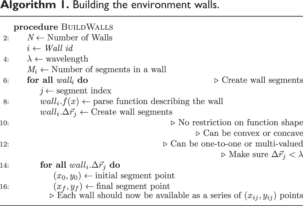
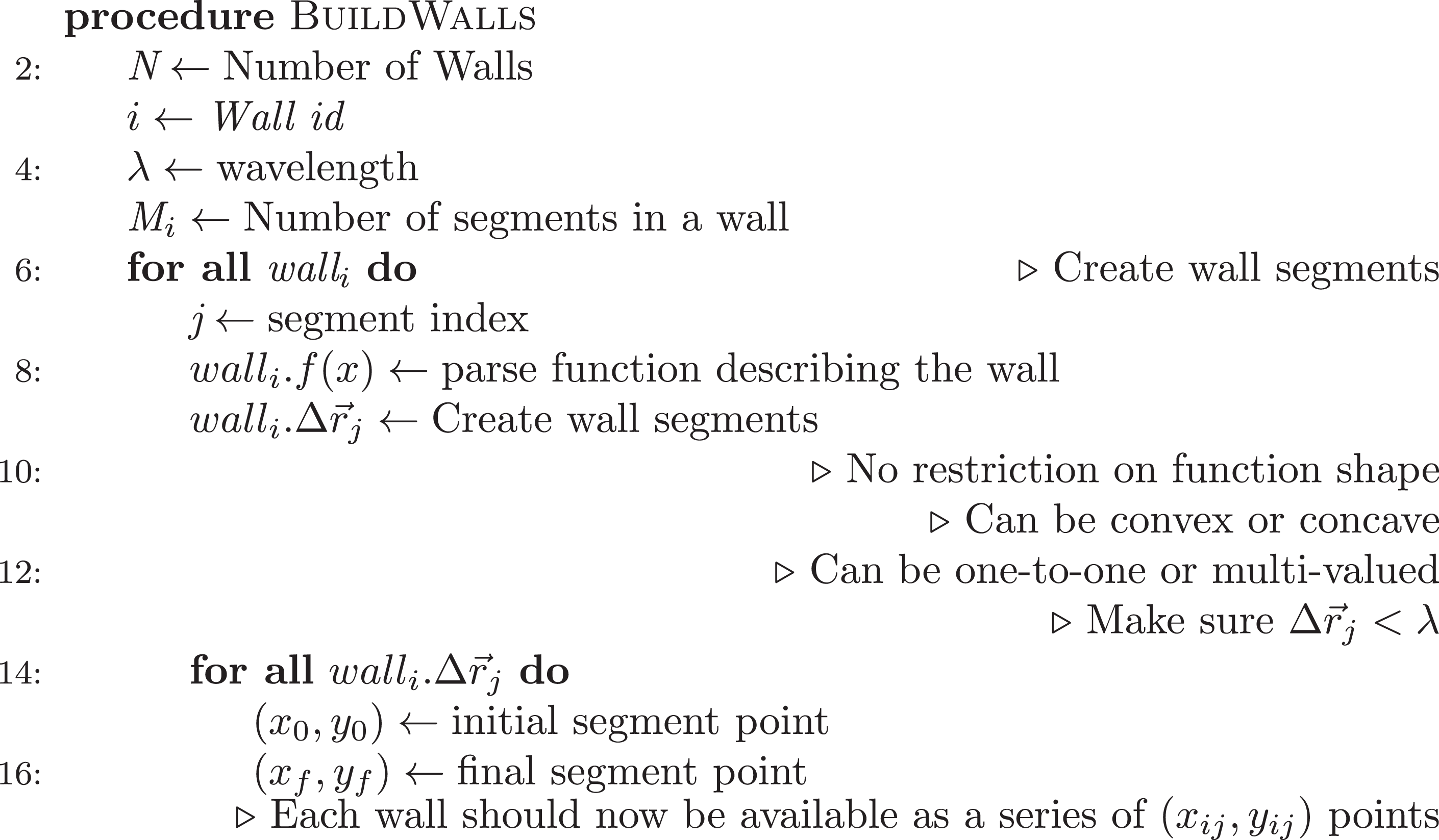
The walls: The simulated 2-D environment is assumed to have a set of smooth walls that do not scatter the incident waves and can be described using mathematical functions such as linear or circular. The number of walls can be very large. Each wall extends over a known range. Since OpenCL 2.0 does not support pointers to functions, nonlinear walls are simulated as a large set of linear adjacent walls. Throughout this work, it was assumed that each nonlinear wall consists of linear segments whose lengths are 10% of the wavelength of the simulated pulse. Assuming 40 kHz ultrasonic waves frequency, dividing a wall into linear segments that are 1 mm long or less is reasonable. All walls are assumed to be identical and reflect all of the incident waves. For the purpose of mapping an environment, such as a maze or a set of walls or even mapping an environment around an autonomous vehicle, taking only the reflections is sufficient in most cases. The algorithm that describes the process of constructing the environment walls is shown in Algorithm 1.
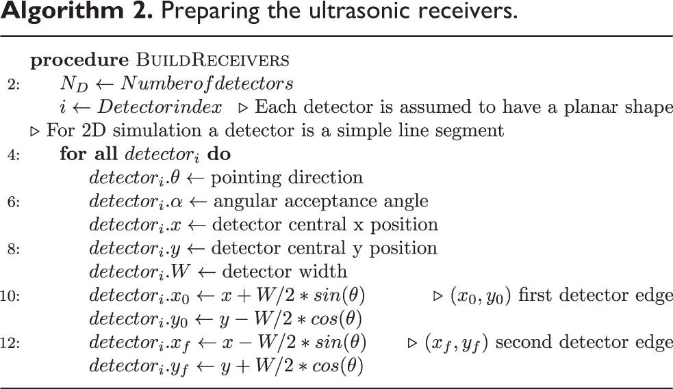
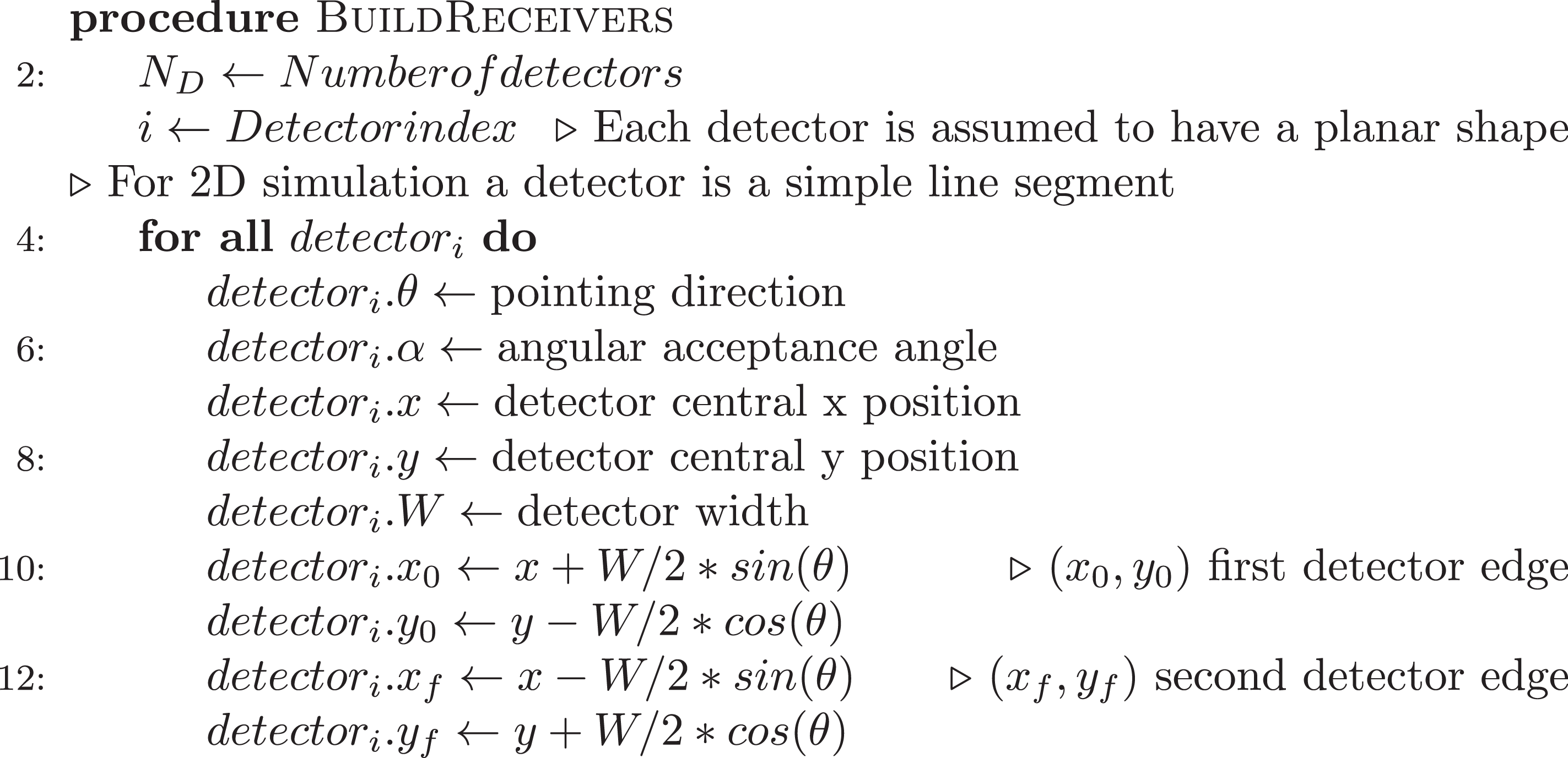
Receivers: The receivers must be located in known locations. Each detector is pointed in a known direction θ and has a known angular acceptance range α as illustrated in Figure 1. In the simulation runs presented in this article, a set of detectors arranged in a circle of about 10-cm radius were used. The ultrasonic pulse source is located at the center of the circle. The ultrasonic receivers’ construction and initialization process is shown in Algorithm 2. The value of the angular acceptance range of a specific receiver depends on its geometrical shape and the effective area facing the incident ultrasonic pulse. The intensity recorded by the receiver Ir
is expected to be
where I
0 is the incident intensity and θ is the angle between the direction of incidence and the normal to the receiver surface. Throughout this work, a set of HC-SR04 ultrasonic transceivers were used. To get better simulation results, the transceivers characteristics were measured. Figure 2(a) shows the measured intensity of the receiver versus its pointing direction. The solid smooth line represents the theoretically expected curve in equation (1), while the dotted one is the experimentally measured normalized intensity. Equation (1) was used to model the receiver behavior throughout this work.
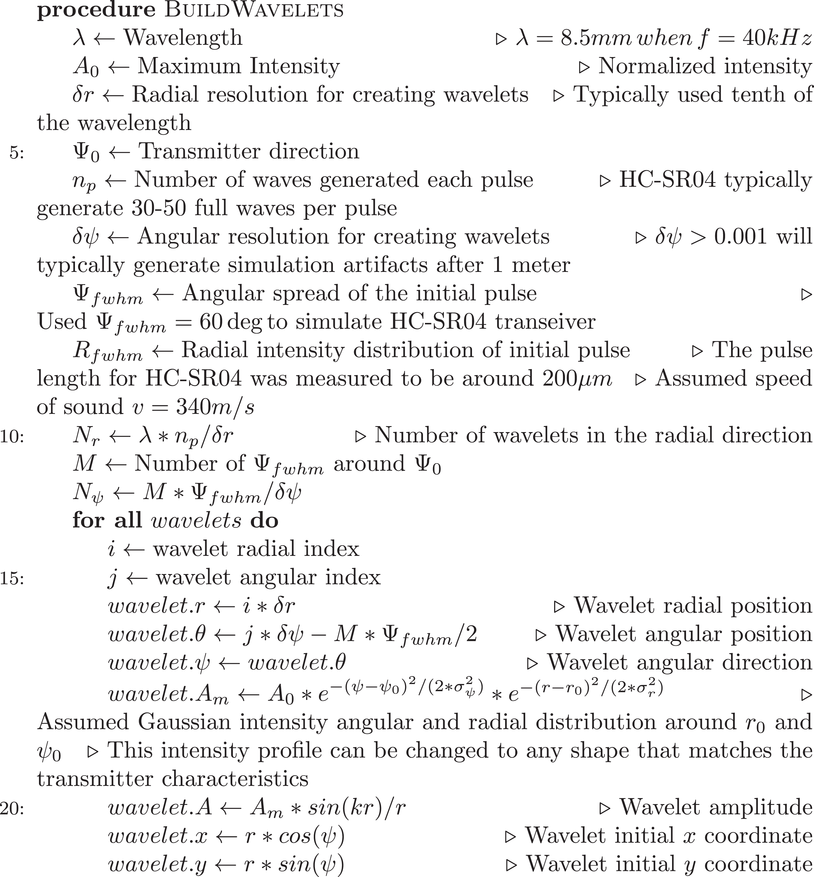
The ultrasonic pulse: The pulse shape is assumed to have an intensity profile similar to common, low cost, commercially available ultrasonic transceivers such as HC-SR04 and HRLV-MaxSonar-EZx. The pulse is assumed to have a 2-D Gaussian shape with a known full-width at half maximum (FWHM). This assumption is driven by the experimentally measured shape of the emitted pulse of HC-SR04 transmitter. The measured angular distribution of the emitted pulse is shown in Figure 2(b), where the dotted smooth curve is the profile used by the simulation program. The amplitude versus time profile of the emitted pulse is shown in Figure 2(c). Since the raw emitted pulse contains several frequency harmonics on top of some noise, the data shown in Figure 2(c) are filtered using a band-pass filter around the nominal 40-kHz pulse frequency. The simulated pulse shape can be changed to any desirable shape to match the transceiver being simulated. The pulse is simulated as a large number of decaying intensity points emitted around the direction ϕj
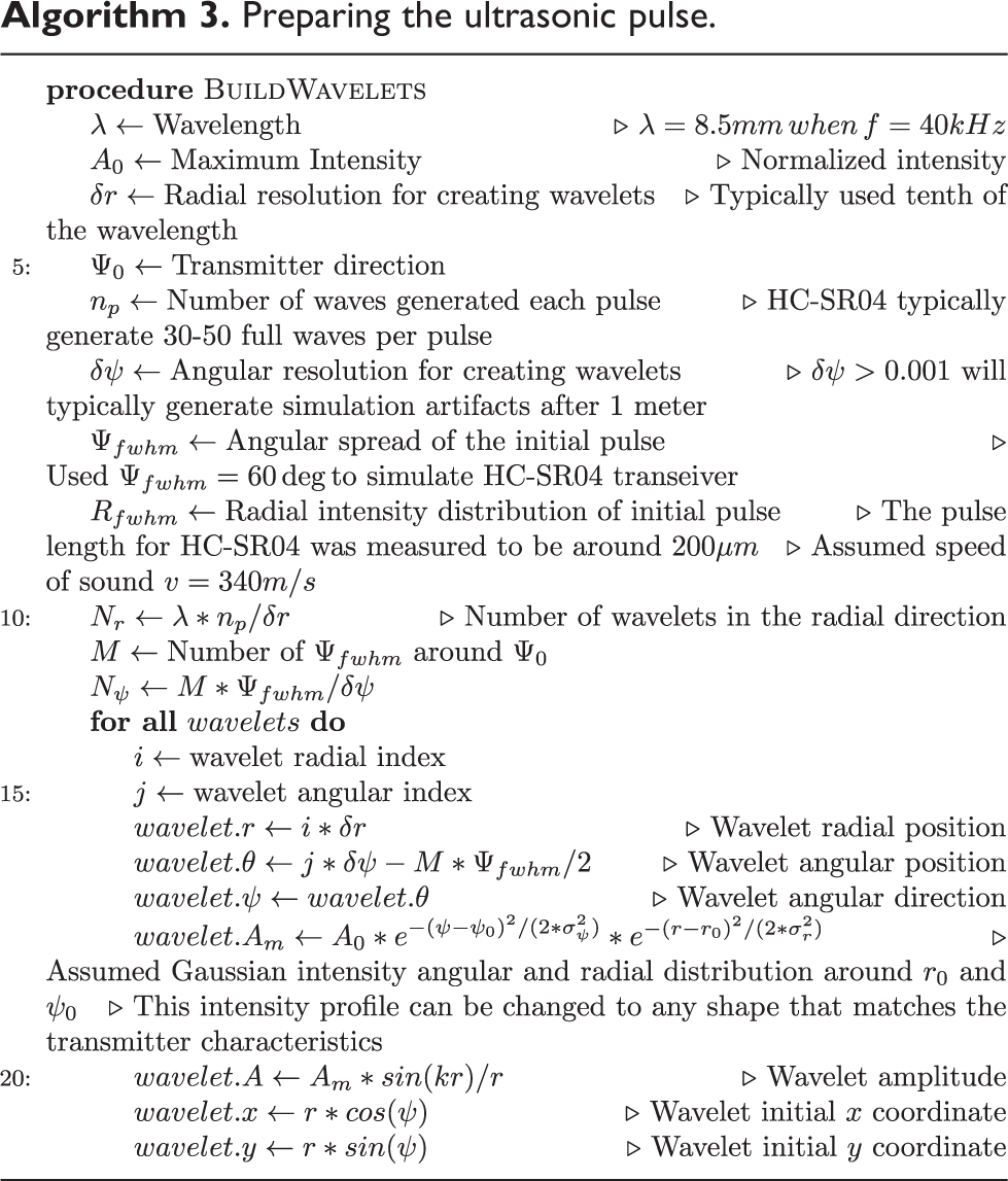
as shown in Figure 1 and has the spatial distribution shown in Figure 3. The pulse shown in Figure 3 will typically contain millions of points or wavelets. This large number of independently propagating wavelets makes using a GPU ideal for performing this task. The wavelets construction and initialization process is shown in Algorithm 3.
Building the environment walls.
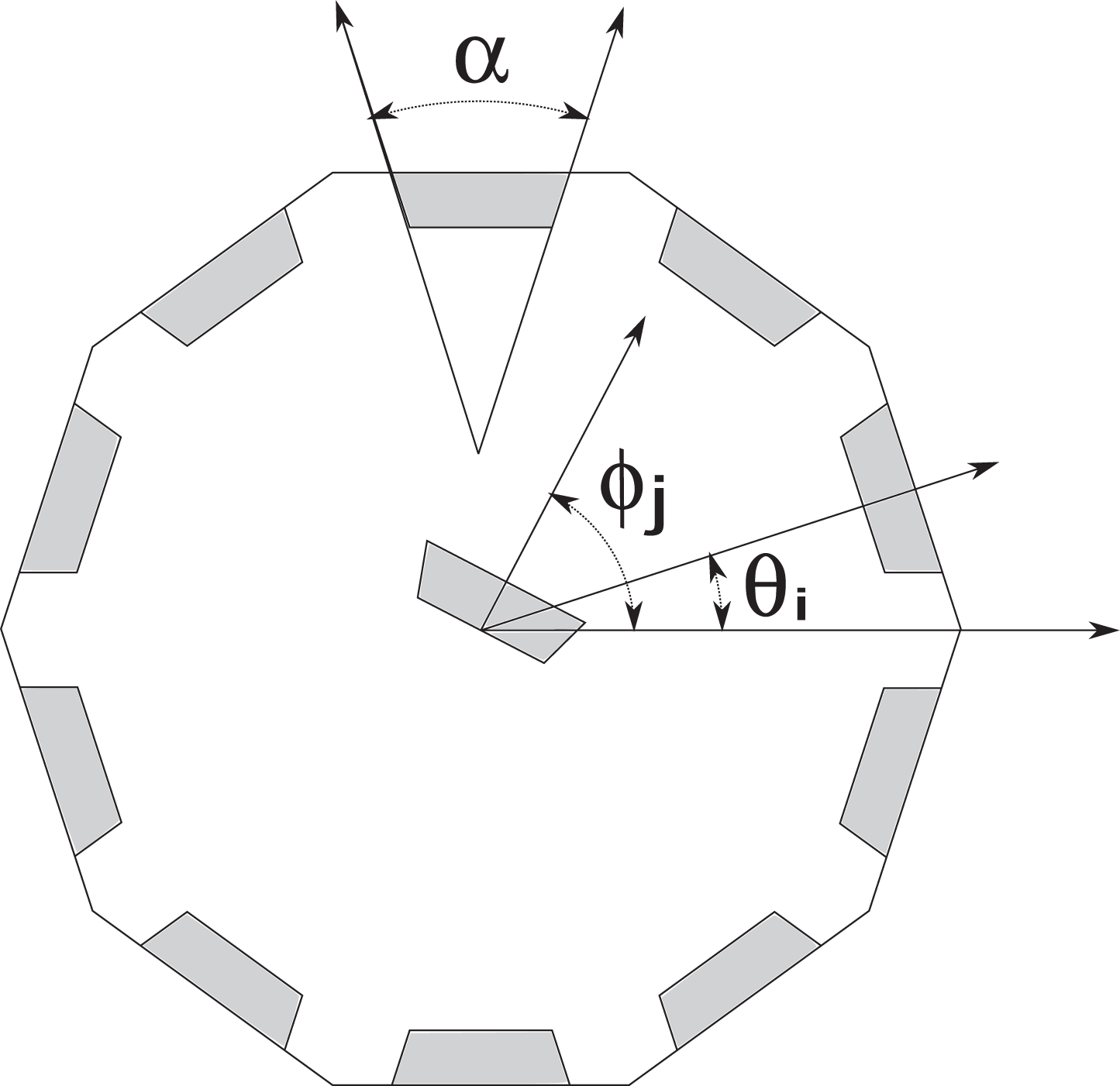
An ultrasonic pulse source is located at the center pointing in the direction ϕj . The receivers are arranged in a circle with known angular positions θi and acceptance angle α.
Preparing the ultrasonic receivers.
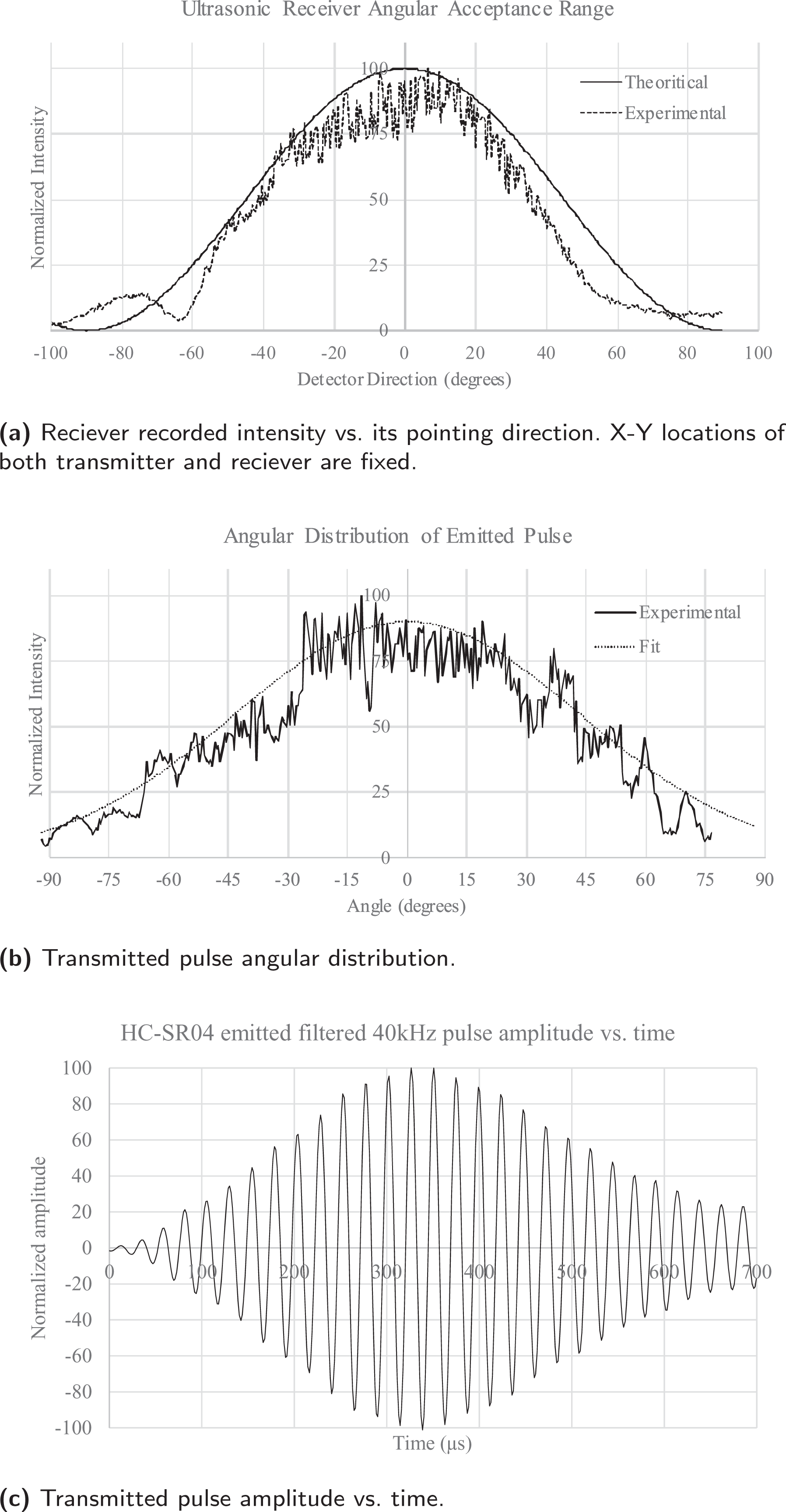
HC-SR04 transceiver characterization. (a) Receiver recorded intensity versus its pointing direction. X–Y locations of both transmitter and receiver are fixed. (b) Transmitted pulse angular distribution. (c) Transmitted pulse amplitude versus time.
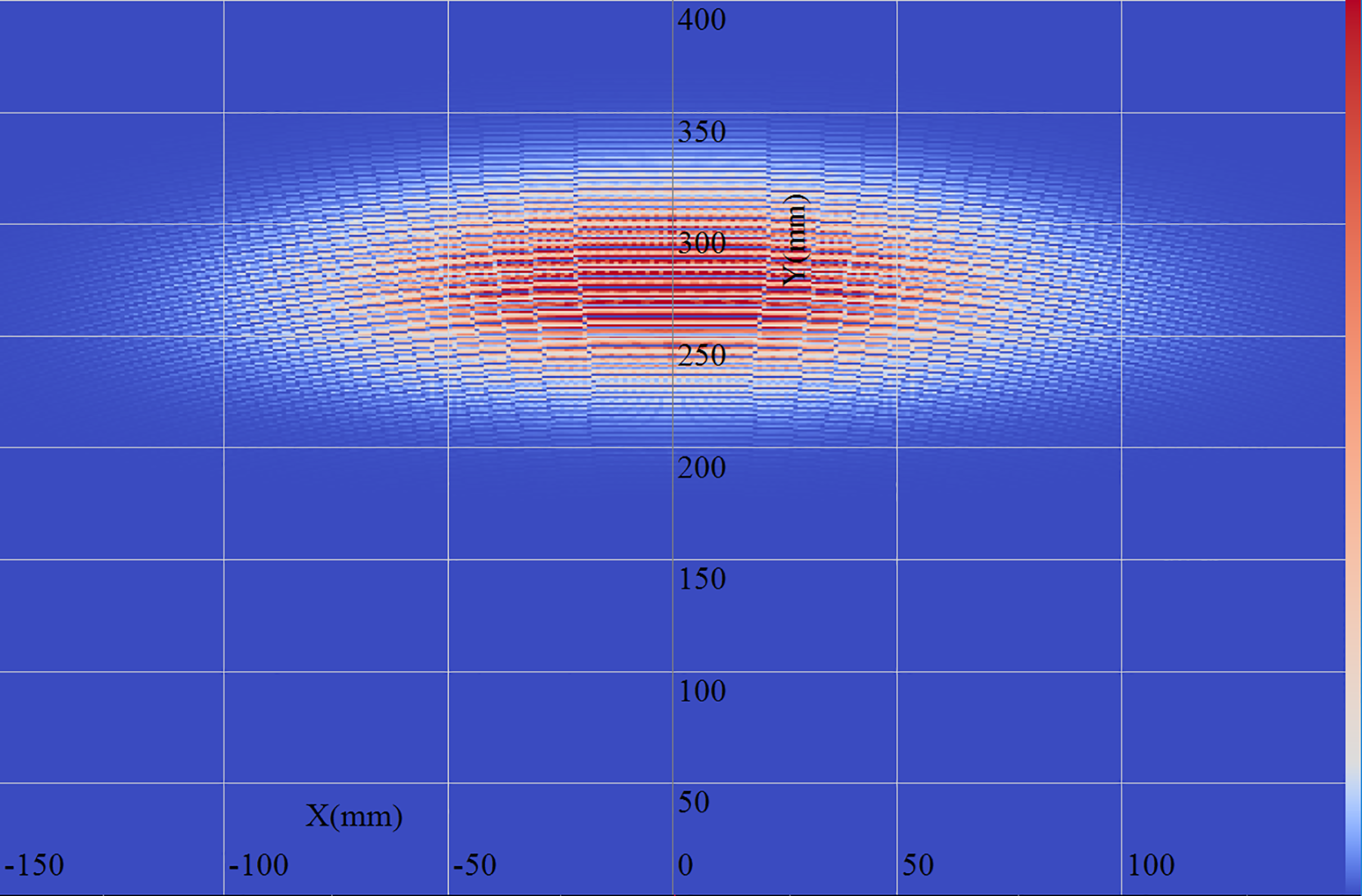
Simulated spatial distribution of the initial ultrasonic pulse generated by a source located at the point (0, 0) after traveling about 300 mm. The logarithm of the intensity is represented using the color scale shown to the right of the figure.
Preparing the ultrasonic pulse.
2.2. Propagating the wavelets
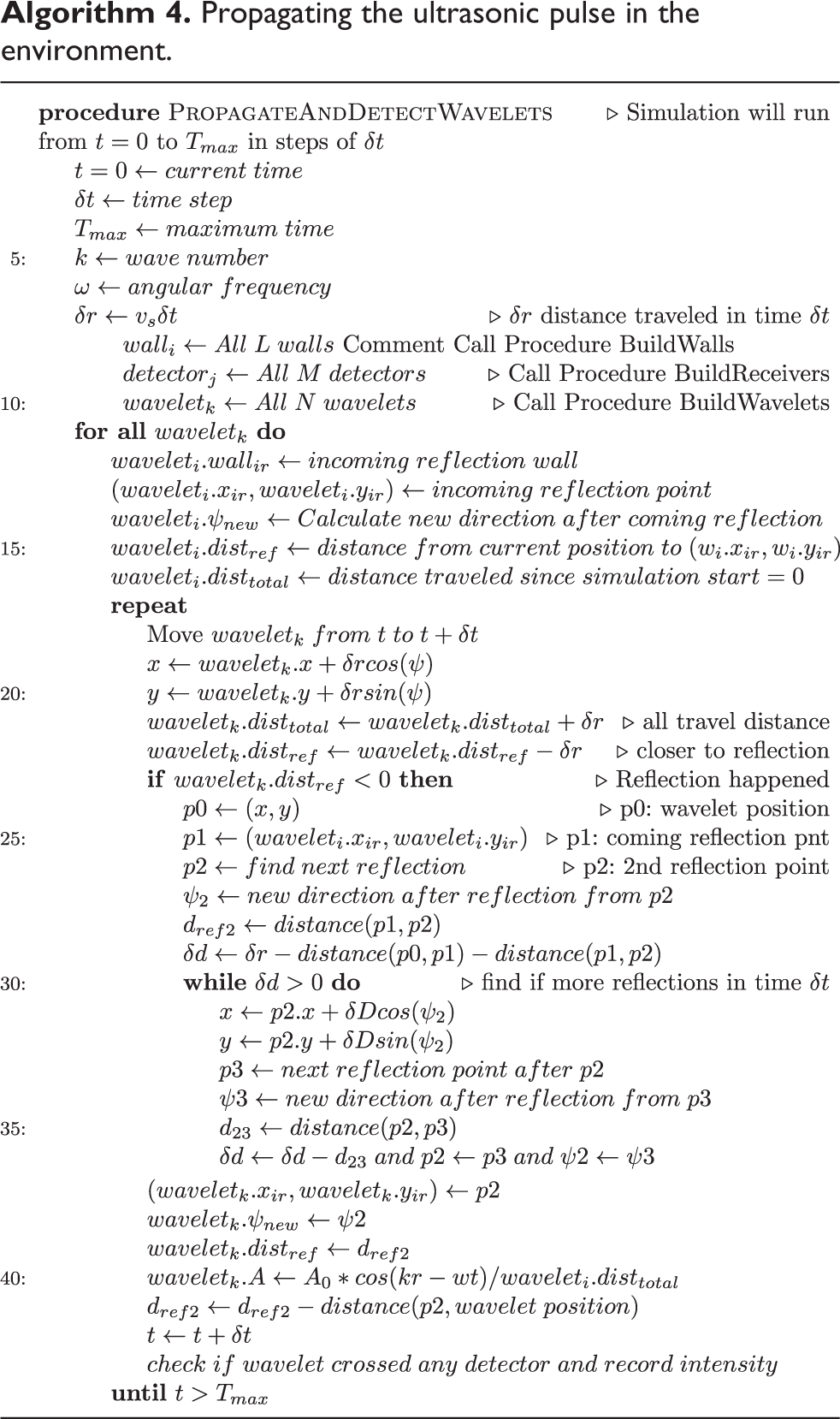
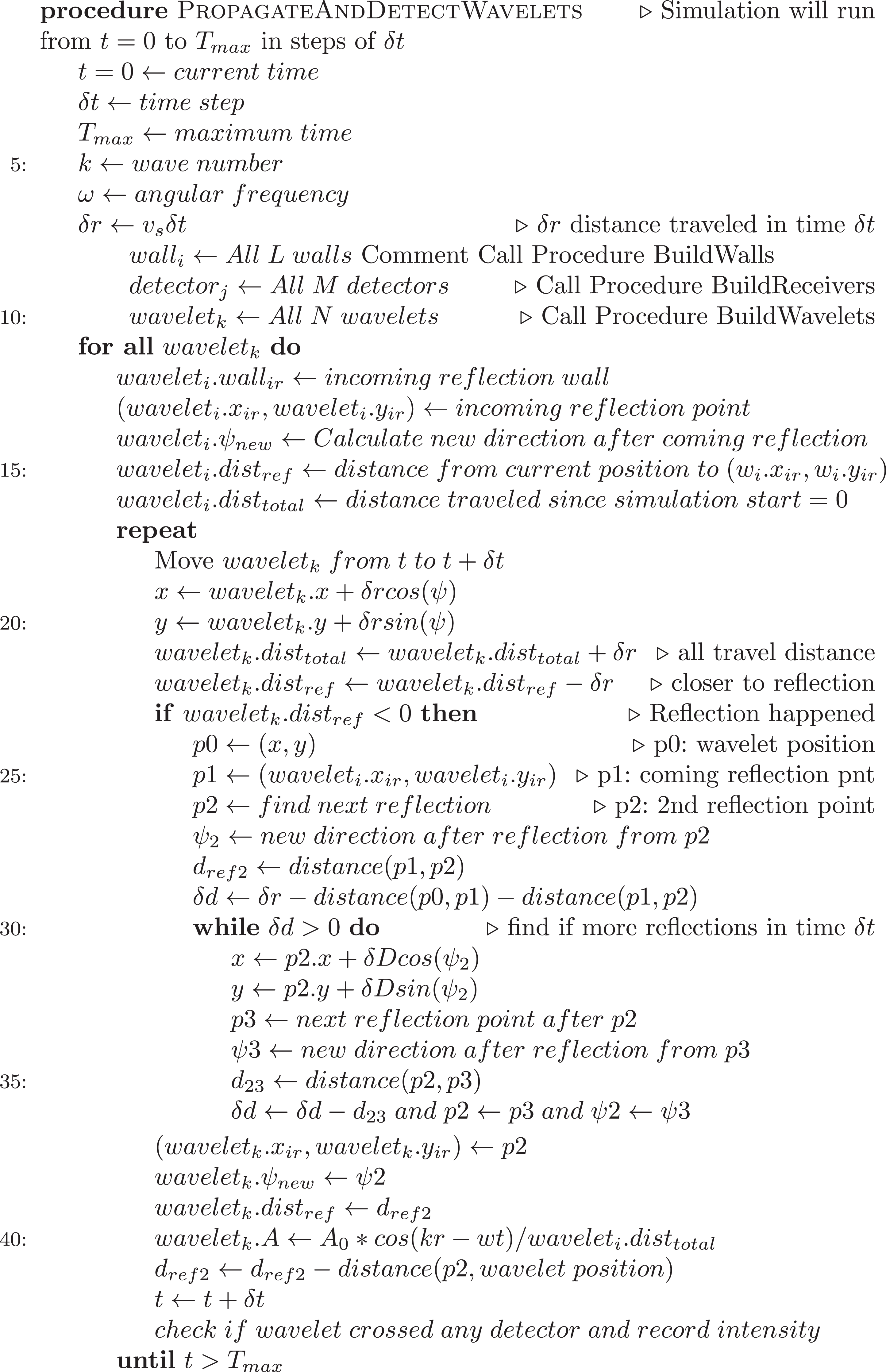
Once the pulse and the surrounding environment are ready, it is time now to propagate all of the wavelets and record the intensity at the detector sites as a function of time. Each wavelet is assumed to move according to the equation
This is the most important part of the code and it will run mostly on the GPU. The algorithm that describes this process is shown in Algorithm 4. The loops shown in the algorithm are parallelized using OpenCL. It is worth noting here that all of the algorithms shown in this article are oversimplified. The actual simulation program consists of about 20,000 lines of code that cannot be described in detail in this limited space. The simulation code will be available from the authors upon request.
Propagating the ultrasonic pulse in the environment.
3. Performance analysis
There are two factors that affect the simulation performance: the system hardware and the simulation parameters. The most important aspects of the system hardware that affect the simulation kernel performance are the GPU 64-bit floating point (FP64) processing power, GPU RAM size and performance, and the PCI-Express bus transfer speed.
In this work, three different AMD Radeon 8 GB PCI-E desktop graphics cards were used. See Table 1 for more details. Although the three GPUs sell for about the same price (US$200–US$250 at the time of writing this article), they have different FP64 theoretical performance and different number of stream processors (SP). What makes the selection of these three cards interesting is that, when configured to run at the same clock speed, they have 125 MFLOPS/SP, 250 MFLOPS/SP, and 500 MFLOPS/SP FP64 processing power, which makes them suitable for studying the simulation FP64 performance. The maximum number of concurrent threads that can be run on each GPU equals four times the number of its SP (N SP). This fact is illustrated in Figure 4 using RX 580 GPU with 2304 SP.
List of GPUs used in the performance analysis.

GPU: graphics processing unit; SP: stream processors.
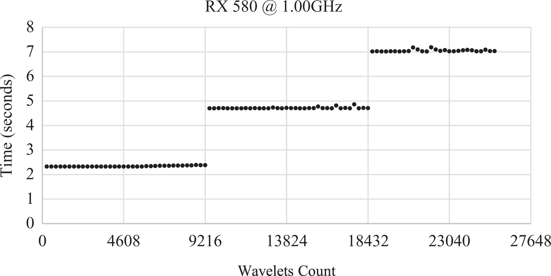
Time to move a number of wavelets 1000 time-steps in the environment shown in Figure 12 using Radeon R9 580 GPU. Core clock speed = 1000 MHz. The number of concurrent threads equals four times the number of stream processors. GPU: graphics processing unit.
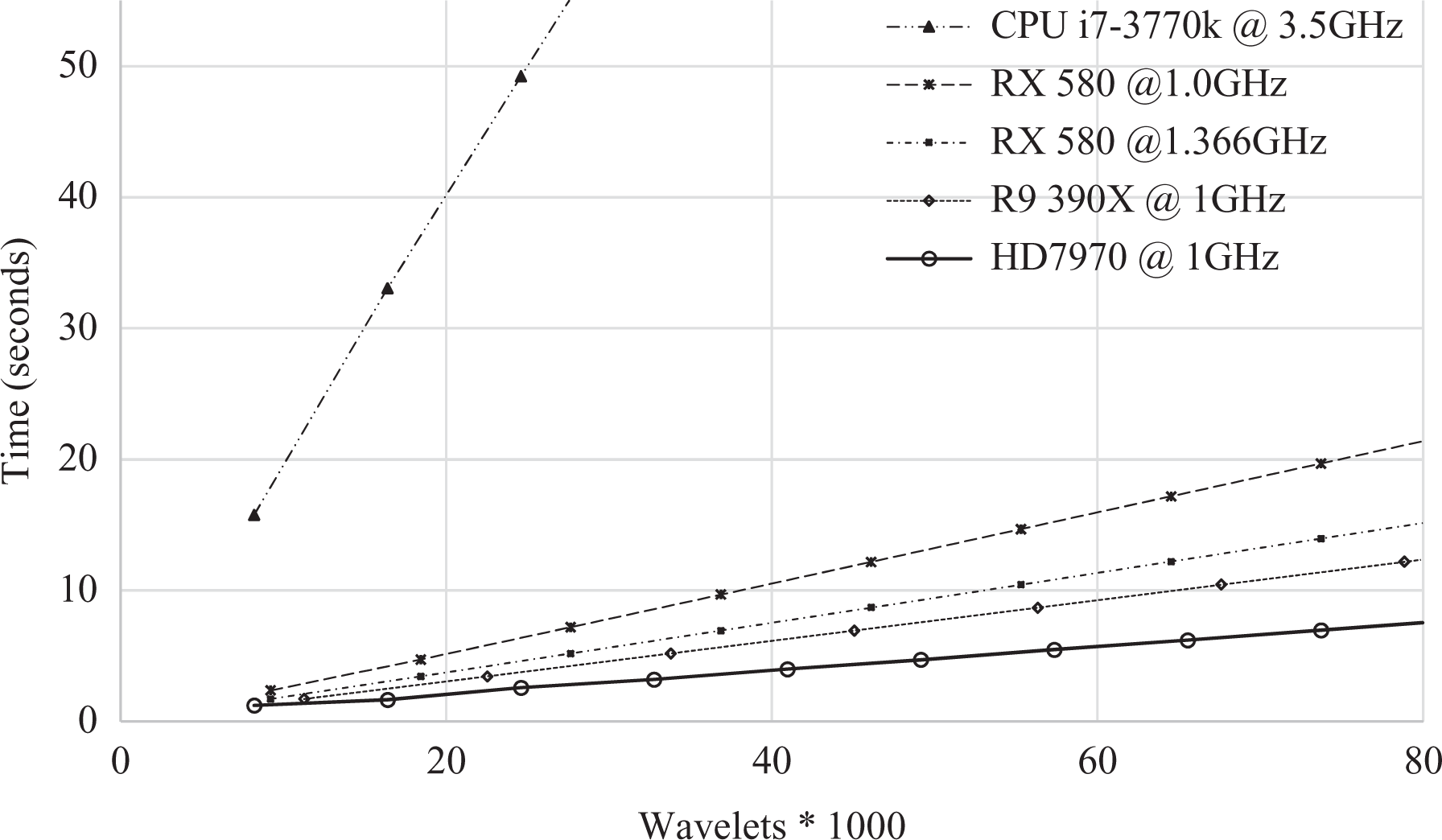
To understand how the simulation performance scales with FP64 processing power, a number of wavelets N
w = n × N
SP, where n is an integer, were moved 1000 time-steps δt = 20 µs on each GPU (T
max = 20 ms). The time to move N
w wavelets 1000 times is then recorded. The results are shown in Figure 5. From the slopes of the lines in Figure 5, the average time to move a single wavelet one time-step δt can be calculated (given
Average time to move one wavelet a single time-step in the environment shown in Figure 12 using four different devices.
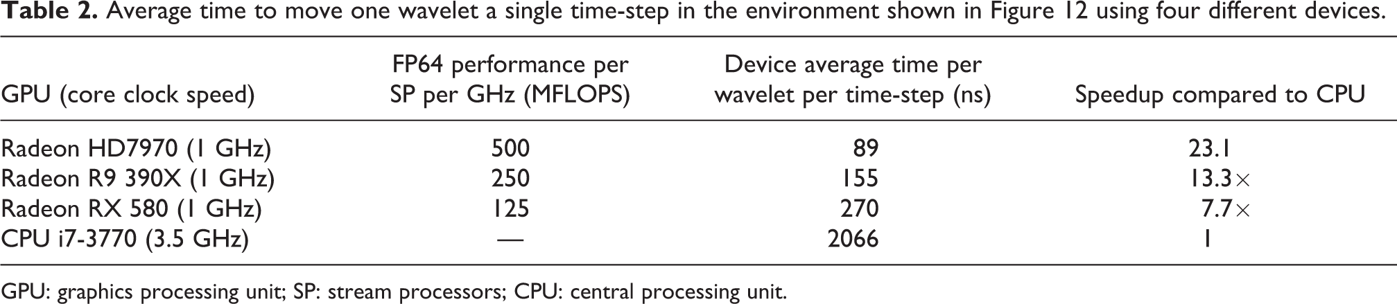
GPU: graphics processing unit; SP: stream processors; CPU: central processing unit.
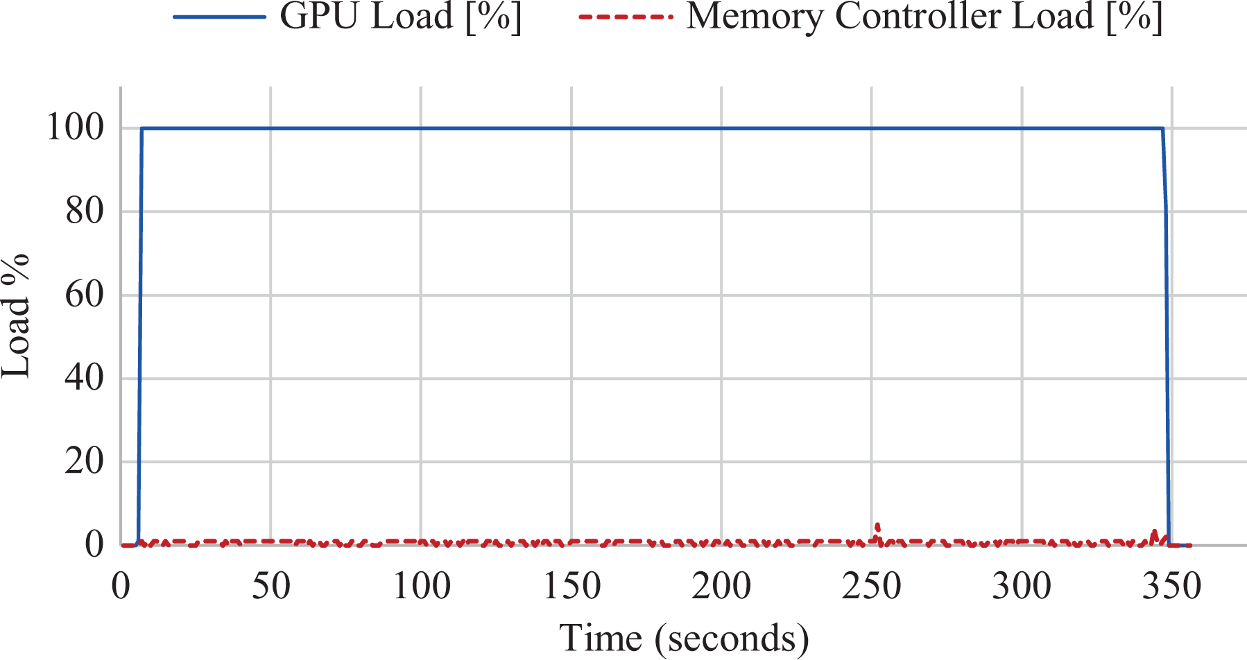
GPU core and memory controller activity while running 6,553,600 wavelets on RX 580 GPU. Core clock speed = 1300 MHz. Data collected using GPU-Z 2.14.0. GPU: graphics processing unit.
Even though the GPU RAM clock speed has little or no measurable impact on the simulation performance, the amount of GPU RAM puts an upper limit on the number of wavelets that can be simulated in a single OpenCL kernel call on one device. In this simulation, all wavelets were passed to OpenCL kernel in an array of C-structs. Since OpenCL compiler automatically aligns structs and unions and basic data types, no additional action was necessary to solve any memory alignment issue on the GPU. Each wavelet occupies 192 bytes which means that an 8-GB GPU RAM can fit about 44 million wavelets. The amount of RAM occupied by the walls and the detectors is ignorable compared to the wavelets RAM. Since a PCI-Express 3.0 ×16 bus has a maximum throughput of 15.8 GB/s, a 44 million wavelets simulation result can be transferred from the GPU in less than a second.
All the used GPUs had a recommended OpenCL local-work-group size of 256 × 256 × 256 for 3-D work groups. Throughout this work, a local-work-group size (threads array) of 256 × 256 or 256 × 1 was used. No performance penalty was noticed as long as
The number of wavelets can be adjusted by changing δψ (the angular separation of adjacent wavelets) and δr (the radial separation). A sufficient number depends on the propagation distance being simulated, as the wavelets diverge with time, and the features that should be resolved in the reflected signal. As a test case for determining a proper value of δψ, a pulse reflected from an obtuse 165° corner that is 1.5 m away will result in two interfering wave fronts at the receiver sites. This will produce diffraction patterns that will not be resolved if δψ is not small enough. The simulation was run repeatedly for δψ = 0.001–0.200°. The reflected pulse intensity versus receiver position is then recorded. All the results are combined in Figure 7. Note how the simulation data for δψ > 0.020° become gradually very noisy. Throughout this article, a δψ = 0.005° was used. This value should be sufficient even at the maximum HC-SR04 transmitter range.
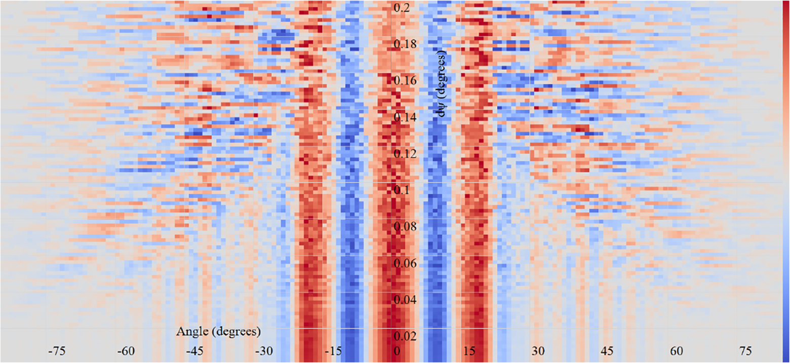
Amplitude (color) versus ultrasonic receiver angular position (horizontal axis) for various values of δψ simulation parameter (vertical axis). The color shown to the right of the figure represents the amplitude: negative is blue and positive is brown-red.
The radial wavelets separation δr is not critical and can be chosen, according to Nyquist theorem, such that
where λ is the pulse wavelength, if any information from the radial direction is needed.
4. Experimental validation
In this section, the design and construction of a test device is presented. The experimental results from the test device are then compared against the simulation results in two test cases. The first test scenario demonstrates the experimental and simulated data sensitivity to subtle changes in angles, while the results from the second test scenario demonstrate the ability to detect an unseen object hiding behind a corner or inside a room.
4.1. Test device
To experimentally verify the output of the simulation, a device that can transmit a pulse in a known direction and listen to the reflections coming from all directions was designed and built (see Figure 8). To simplify this device, as currently its only purpose is to verify the simulation results, two HC-SR04 ultrasonic transceivers were used. One of them was modified to work only as a receiver and the other one as a transmitter. This modification was done by disabling the corresponding piezoelectric element in each transceiver. The transmitter was mounted on a frame that has a stepper motor attached to it, and the receiver was mounted at the end of an arm that can be rotated by the stepper motor. Ideally, a test device should be able to listen to the ultrasound coming from all possible directions as illustrated in Figure 1. Using the setup shown in Figure 8, one had to repeatedly send the same pulse in the same direction and listen to the reflected intensity–time profile at different angles θi (see Figure 1).
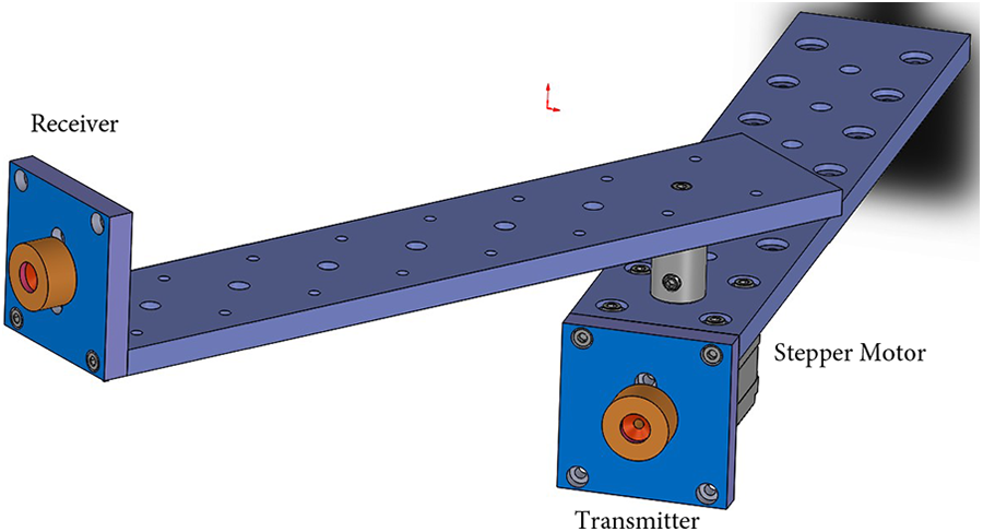
Experimental setup 3-D model.
The stepper motor, which has 400 steps per revolution, was driven using a motor driver that can divide each step into 50,000 steps. During the performed tests, the receiver position was rotated by 0.1° after listening for 10–30 ms after each transmission.
The data acquisition and control of the various components was performed using Atmel SAM3X8E ARM Cortex-M3 84 MHz microcontroller unit (MCU) that has 12-bit analog-to-digital converter with one mega sample per second conversion speed. At 40 kHz ultrasound frequency, this sampling rate meant that one can sample a full wave using about 28 points. The collected intensity–time profiles were saved using a flash-memory storage unit connected to the MCU.
4.2. First test environment
The first test environment walls design is shown in Figure 9. Note that the transmitter is rotated 2.5° ± 0.1° clockwise with respect to the line that divides the angle 78.5° ± 0.1° in half. The reason behind the choice for the angles shown in Figure 9 is to illustrate the sensitivity of the device. The scan angle θ in Figure 9 was changed from 0.0° to 180.0° in steps of 0.1°. The experimental data for the setup in Figure 9 are shown in Figure 10(a), and the simulated data for the same setup are shown in Figure 10(b). The colors in the figures represent the normalized intensity logarithm. The used color scale is shown to the right of each figure. The color scale is chosen such that the background, including the noise, is in blue, while the usable signal is in brown-red. After comparing the two sets of data, one can note the following: Both data sets have the same overall shape: There are three reflected wave fronts. The strongest one is the result of direct reflection from the wall in front of the transmitter. The other two wave fronts located around θ = 90°, t = 2900 µs and θ = 185°, t = 3300 µs are the result of a second-order reflection from the middle wall to the side walls and then to the receivers. Because of the 2.5° noted previously, the wave front at θ = 90°, t = 2900 µs arrived 410 µs earlier. To illustrate this difference, the two peak intensities were integrated over their respective angular range, and the integrated intensity versus time was plotted, for both the experimental and the simulated data. The normalized integrated intensity is shown in Figure 11(a) for the simulated result, and in Figure 11(b) for the experimental one. The fitted location of the peaks in Figure 11(a) is t = 3339 ± 2 µs and t = 2925 ± 2 µs, respectively, with a difference of 414 µs, while the fitted location of the peaks in Figure 11(b) is t = 3327 ± 2 µs and t = 2924 ± 2 µs, respectively, with a difference of 403 µs. This 2.6% difference is mainly due to the error in measuring the wall angles in Figure 9. Such features in the collected data can be used reliably to discover the properties of an unknown environment walls such as an angle between two walls even if they do not intersect, or the slope/tilt of a wall, or even its curvature. The feature located at θ = 135°, t = 900 µs in Figure 10(a) is due to reflections from the device itself and can be safely ignored. The band in Figure 10(a) around t = 4200 µs, and covering all angular positions, is caused by the reflected wave fronts hitting the device body and finding their way to the receiver, through the instrument body, regardless of the receiver arm pointing direction.
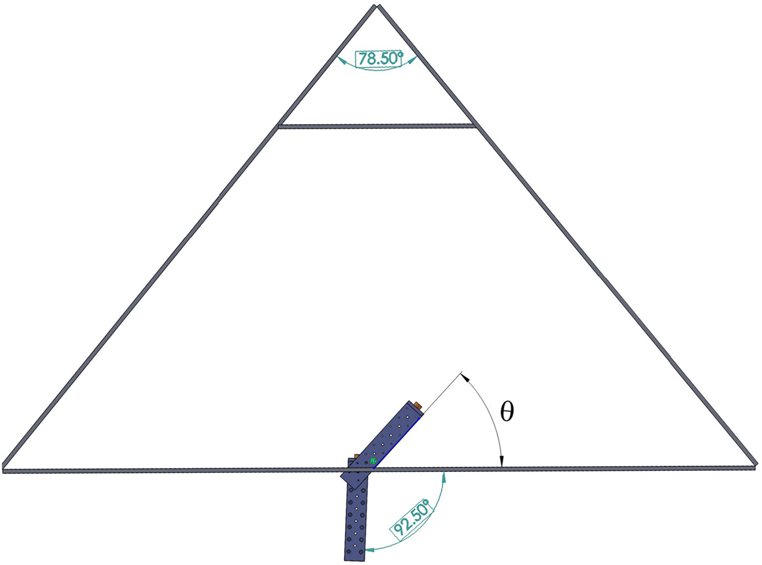
Test environment geometry.
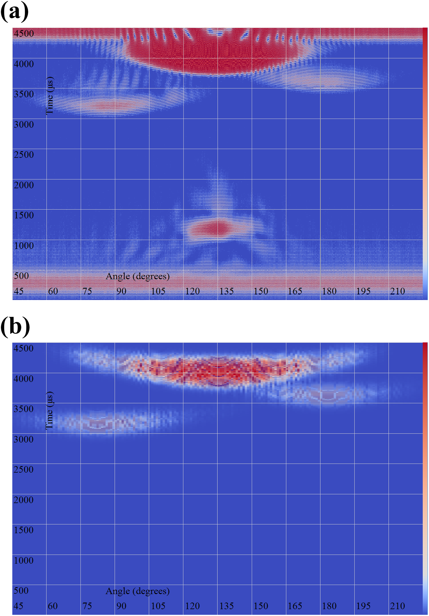
Experimental versus simulated results for emitting a pulse toward the environment shown in Figure 9. Simulation parameters δΨ = 0.005°, Ψ
fwhm = 90°, δr = 2 mm, δt = 3 μs, N
λ = 20 full waves, R
fwhm = 80 μs, and
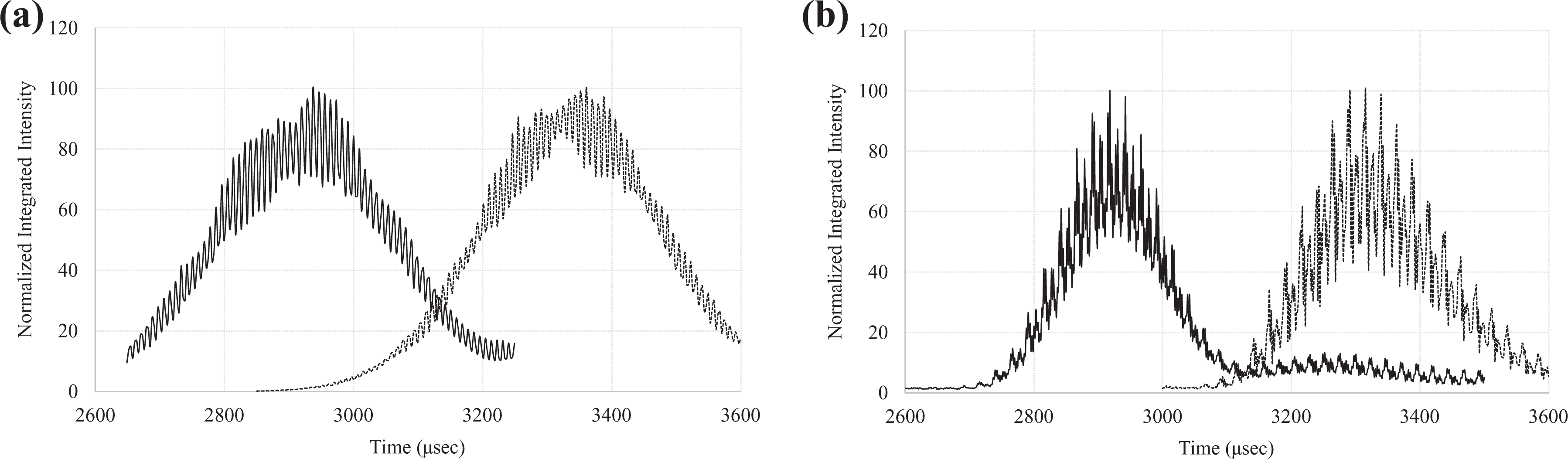
Normalized intensity integrated over the angular ranges of the reflected wave fronts at θ = 90°, t = 2900 µs and θ = 185°, t = 3300 µs in Figure 10(a) and (b), respectively. (a) Simulated data and (b) experimental data.
4.3. Second test environment
The second test environment design is shown in Figure 12. It contains a 53 × 50 cm2 space at the upper-left corner that cannot be seen directly from the marked device location. The probing pulse was directed 30° with respect to a horizontal axis in Figure 12. The reflected echoes were collected with, and without, a 55-mm diameter cylindrical object placed in the center of the 53 × 50 cm2 space. These two test cases will be discussed in the next two subsections.
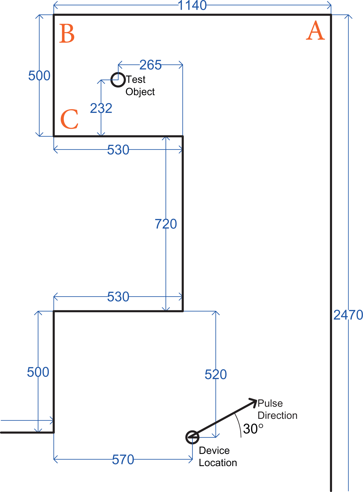
Second test environment design. All dimensions are in millimeters.
4.3.1. Case 1
In this case, the test environment is as shown in Figure 12, but without the test object. Figure 13(a) and (b) shows the experimental and simulated data, respectively. To demonstrate the simulation accuracy, the positions and shapes of the reflected echoes will be compared. Table 3 lists the strongest 11 reflections, or echoes, and compares their average arrival times. The average error in predicting those times is 2.45%. This error is mainly due to the ±1 cm in the walls and device placement using a meterstick. Since the distance traveled by a wave is D = vt, where v is the constant speed of sound, an error in the walls/device placement is linearly proportional to the error in the reflected wave front arrival time.
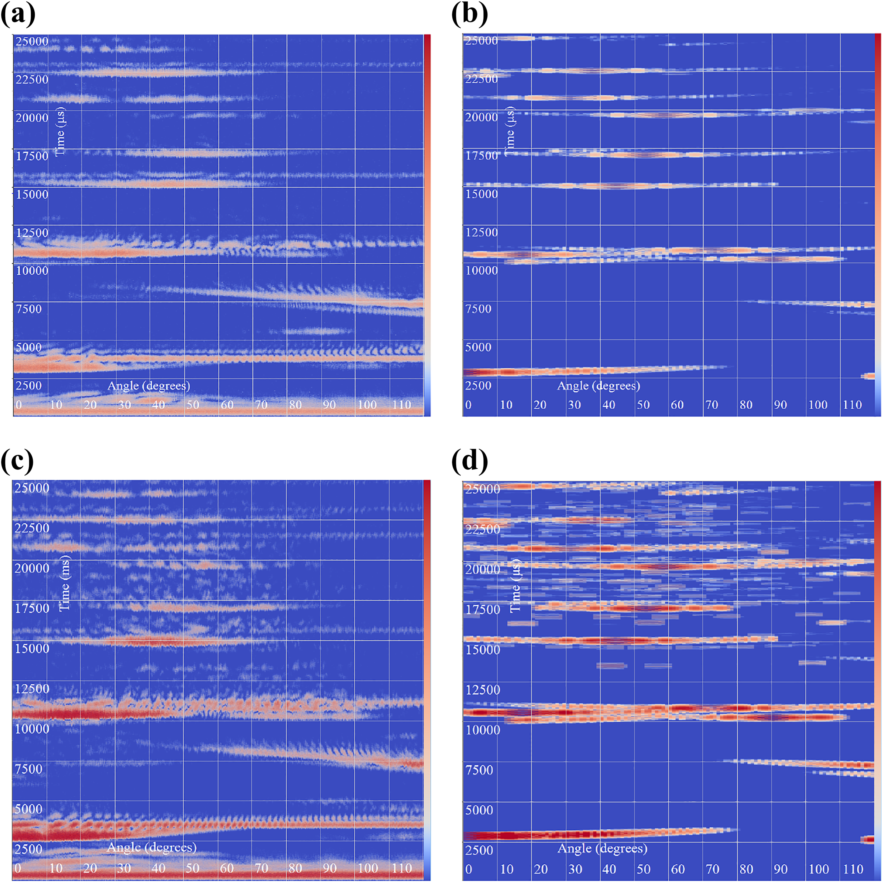
Experimental versus simulated data for propagating an ultrasonic pulse in the environment shown in Figure 12 with, and without, the test object. Simulation parameters δΨ = 0.005°, Ψ
fwhm = 90°, δr = 2 mm, δt = 3 μs, N
λ = 20 full waves, R
fwhm = 80 μs,
Experimental versus simulated data.a
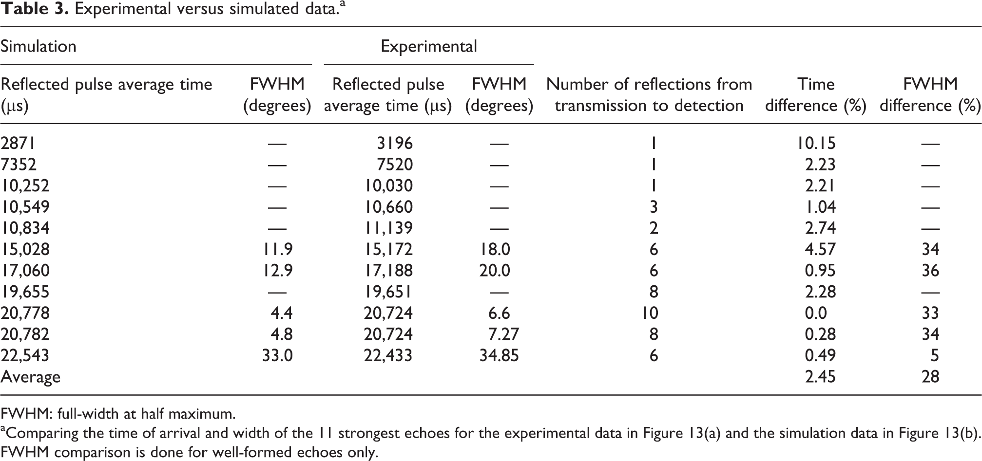
FWHM: full-width at half maximum.
aComparing the time of arrival and width of the 11 strongest echoes for the experimental data in Figure 13(a) and the simulation data in Figure 13(b). FWHM comparison is done for well-formed echoes only.
Another aspect of the reflected echoes is their spread across the detectors circle. After plotting a specific echo intensity versus detector location, the FWHM of the well-formed reflections were measured and compared. The results are shown in Table 3. Note that the experimental echoes FWHM are always wider than the simulated ones. This is due to the factors that are not included into the simulation such as scattering and surfaces roughness.
It is worth noting here that the exact shape of a reflected echo depends on at least one aspect of the environment. For example, the echo at t = 15,028 µs depends primarily on the value of angle A in Figure 12, the echo at t = 17,060 µs depends on the value of angle C, and the echo at t = 19,655 µs depends on the value of angle B.
4.3.2. Case 2
In this case, the test environment is as shown in Figure 12 with the cylindrical test object present. The experimental and simulated results are shown in Figure 13(c) and (d), respectively. Note that the environment walls response is similar to the previous case with the additional object signature added to the whole response. In this case, the cylindrical object scatters the incident wavelets in all directions resulting in the sparse spots appearance in the experimental and simulated data. One can analyze the data of this case in a way similar to the previous test case and learn how to infer, for example, the location of the test object, but that is beyond the scope of this article.
5. Conclusion
An ultrasound simulation program that runs on a GPU using OpenCL 2.0 compute language was developed and tested. The program assumes that an ultrasonic pulse consists of a large number of moving wavelets, and it tracks the intensity recorded by a set of receivers with known characteristics and locations. The program does not impose any restriction on the environment shape. The error in predicting the timing of an echo was around 2.5%, while the error in predicting its angular spread was around 30%. The echoes timing error was mostly due to the positional accuracy of the environment walls, while their angular spread error was due to scattering and walls roughness.
The simulation performance was limited by the FP64 processing power of the used GPU. It took about 10 s to propagate one million wavelets for 1 ms using a $200 desktop GPU. Memory transfer overhead through the PCI-E bus was ignorable compared to the computation time on the GPU. The used GPU performance was up to 23 times faster than a similarly priced CPU using the same OpenCL implementation.
Initial results suggest that the simulation can be used to develop criteria to discover an unknown environment. This could be of utmost importance for many systems such as autonomous vehicles while parking or making a turn into a directly unseen environment. The ability to run such a simulation on a GPU, and get a result within few seconds, enables generating large sets of data for teaching a neural network for the purpose of making an environment discovery robot.
Footnotes
Declaration of Conflicting Interests
The author(s) declared no potential conflicts of interest with respect to the research, authorship, and/or publication of this article.
Funding
The author(s) received no financial support for the research, authorship, and/or publication of this article.
