
Abstract
This article derives analytical solutions for steel pipelines subjected to combined bending moments, axial forces, and internal pressure by considering the effect of ovalization on the plastic region. Both lower and upper bound solutions are proposed based on the selection of a general modulus of pipe material. The ultimate bending capacity, as well as the moment–curvature relationship, can be obtained from the analytical solutions. A comparison of the analytical solutions with the experimental and numerical results finds the bending capacities and the moment–curvature curves in good agreement. Therefore, the proposed analytical solutions can be used to study the behavior of steel pipelines subjected to combined loadings.
Introduction
Buried pipelines are typically subjected to complex loading combinations of internal pressure caused by the actions of the fluids they convey, the axial forces due to thermal and Poisson ratio effects, and the bending moments induced by differential soil movements that may result from seabed movements, seismic activities, frost heaves, and thaw settlements (Emamgheiss, 2007; Palmer and King, 2004; Sen, 2006). Consequently, the study of the bending moment capacities and deformational characteristics of steel pipes under combined loadings is highly significant.
Extensive research has been conducted on the theoretical study of the bending moment capacity of steel pipes under combined loads. Brazier (1927) derived an analytical solution for the ultimate capacities of pipes under bending moments by considering the effect of ovalization. Gerard and Becker (1957) provided a number of interactional relationships for pipes under various loading combinations, which was applicable for pipes with large diameter-to-thickness ratios. Mohareb and Murray (1999), Mohareb et al. (2001) proposed an interactional expression concerning internal pressure, axial forces, and bending moments without accounting for the effects of ovalization and local or global instability. Hauch and Bai (2000) derived an analytical solution for the ultimate capacity of pipes subjected to combined loads by adopting the interaction criterion of multi-axial stresses proposed by Galambos (1998) and considering isotropy in the longitudinal and circumferential direction. Subsequently, Mohareb (2002, 2003) developed general plastic interaction equations for pipes under axial forces, torsion, biaxial bending moments, biaxial shear forces, and internal or external pressure by the lower and upper bound theorems. Schaumann et al. (2005) derived an analytical solution for pipes subjected to combined internal pressure and bending moments based on the equilibrium differential equation of beams. Using elastic-perfectly plastic, linear hardening and power hardening models, Li et al. (2009) suggested analytical solutions for perfect pipes subjected to combined pressure, axial forces, and bending moments.
In the above studies, the effects of ovalization of pipe cross-sections and local buckling on bending capacity are ignored. In addition, fully plastic resistances are reached along the cross-section of steel pipes subjected to bending moments. These simplifications and assumptions seem inappropriate, particularly for pipes with large diameter-to-thickness ratios. Referring to the theory of Mohareb (2002, 2003) and Hauch and Bai (2000), and considering the effect of the ovalization of the plastic region, analytical solutions are thus derived for steel pipelines subjected to combined bending moments, axial forces, and internal pressure.
Basic assumptions and equations
Basic assumptions
To obtain the analytical solution of the ultimate bending capacities for pipelines under internal pressure, axial forces, and bending moments tractable, the following assumptions are introduced:
For a pipe that attains its ultimate bending capacity, a portion of the cross-section is elastic, while the remaining portion is plastic. Any effect of strain hardening in the plastic area is ignored.
The cross-section of the pipeline remains plane both before and after bending so that a plastic neutral axis exists and divides the cross-section into compressive and tensile regions.
The pipeline is considered to be a thin-walled structure. Radial stress and shear stresses are ignored.
The effect of strain localization is ignored.
Because the curvature radius
The yield region of the cross-section is simplified as an arched beam.
Basic equations
Based on the maximum distortional energy density yield criterion, that is, the von Mises yield criterion (Boresi and Sidebottom, 1985), a given point on the pipe section reaches yield when the following condition is satisfied
where
Stress component acting on pipe.
For pipelines subjected to combined internal pressure, axial forces, and bending moments, the radial stress

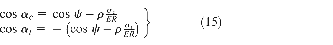
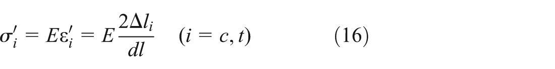
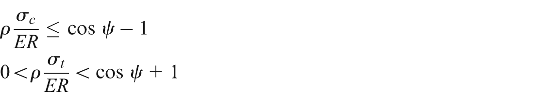
Based on the first assumption in section “Basic assumptions,”equation (2) can be solved to obtain the following expressions for the longitudinal limit compressive and tensile stress
where
Analytical solution for bending capacity under combined loadings
The inward stress components
The main characteristic of a pipeline under bending is the ovalization of its cross-section due to the inward stress components
Ovalization mechanism and inward stress components.
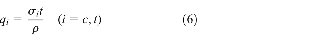
The inward stress components
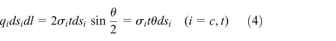
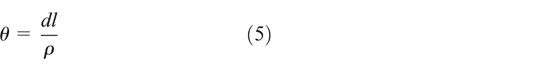
where the subscripts c and t represent the compressive and tensile regions, respectively;
According to equations (4) and (5), the inward stress component
The influence coefficient of ovalization on pipe bending moment
At the initial stage of pipe bending, the curvature radius
Deformation of pipe cross-section under inward stress.
Under the inward stress components, the points
Simplified structures of the plastic regions: (a) compressive plastic region and (b) tensile plastic region.
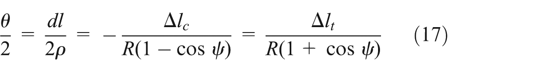
Based on Castigliano’s first and second theorems (Hibbeler, 2005), the vertical displacements

where
The vertical displacements
where
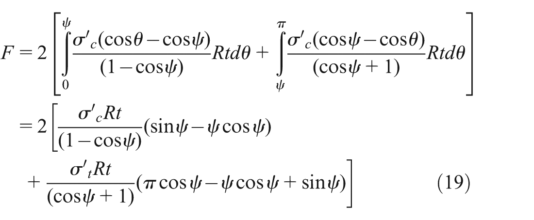
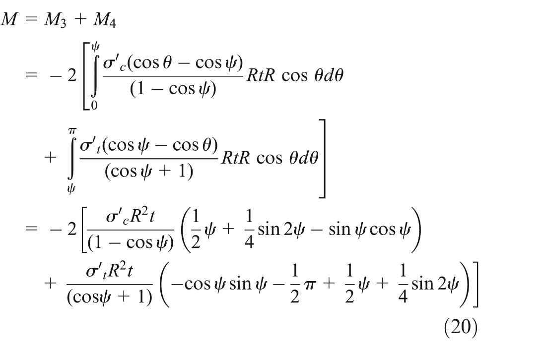
Based on the parallel axis theorem, the bending moment of the plastic region can be divided into two parts: one is the moment of the plastic region with respect to the straight line
where
Substituting equation (8) into equation (9), the bending moment
In equation (10),

where
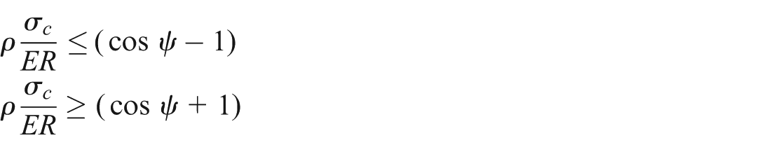
Based on the principle of minimum potential energy (Callen, 1985), there is no concave deformation for a pipeline in a stable equilibrium state under a combined internal pressure, axial forces, and bending moments. Thus, when the influence coefficient is less than zero, that is,
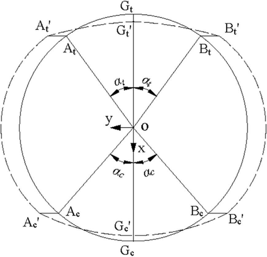
The relationship between the neutral axis and plastic regions
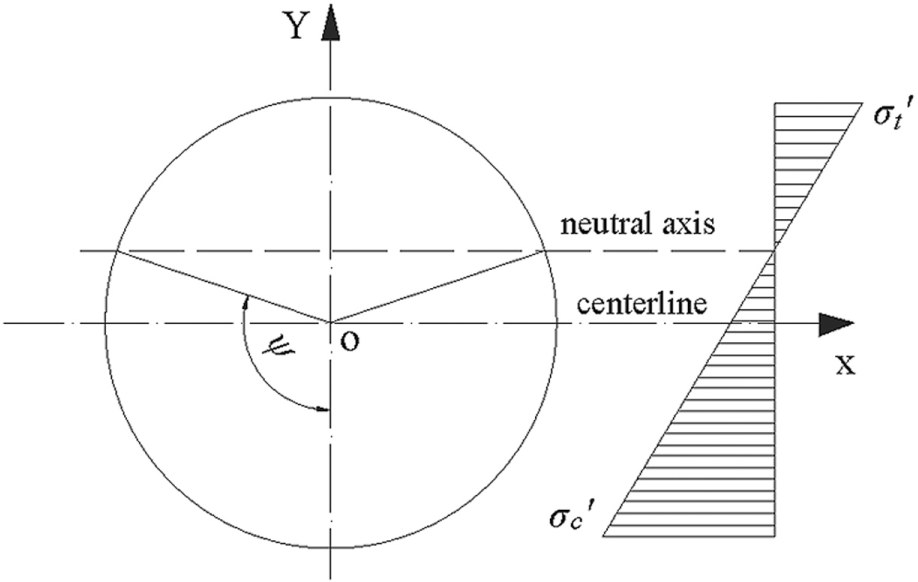
To determine the bending moment applied to a pipe section for a given curvature radius
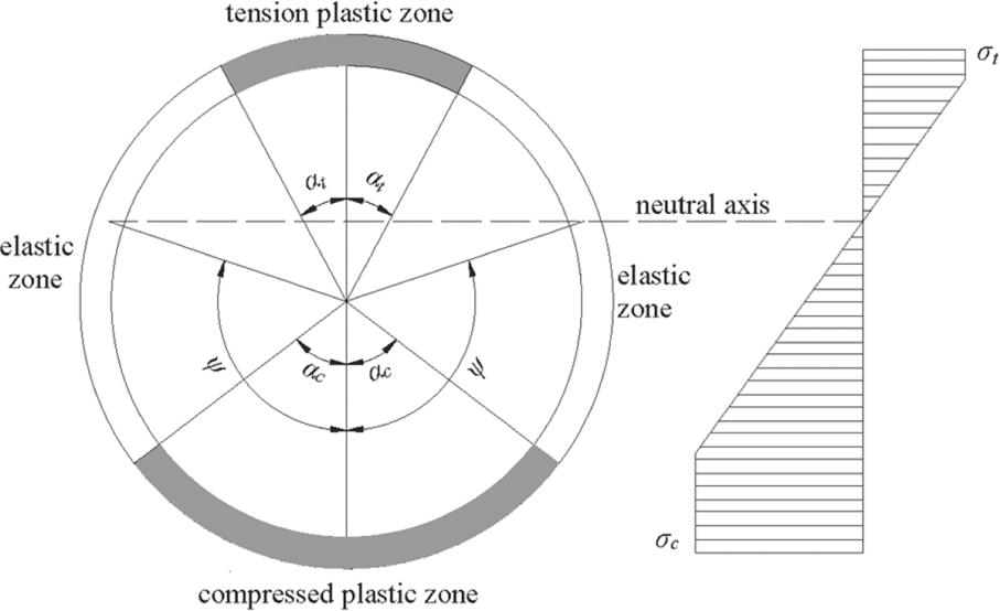
General stress distribution of the pipe cross-section.
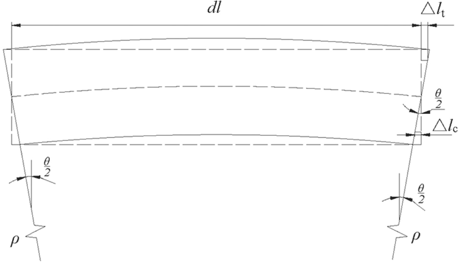
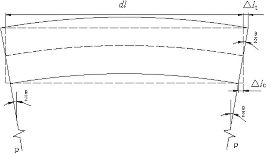
General pipe deformations along the axial direction.
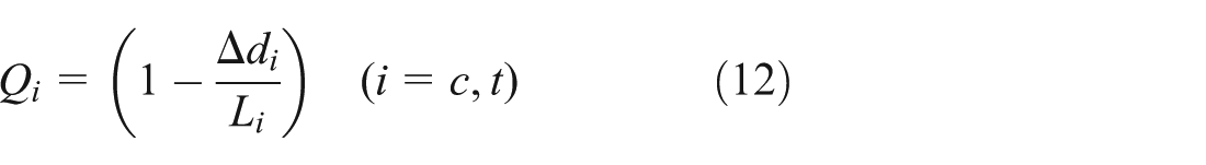
Based on Figures 5 and 6, the following equations can be obtained
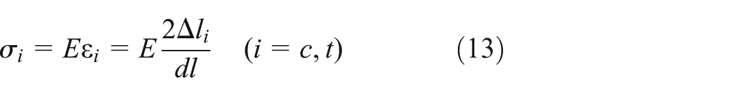

where E is the elastic modulus of the pipeline;
From equations (13) and (14), the relationship between the neutral axis angle
Determination of the pipe bending moment
For a given curvature radius
Case 1
This case indicates that the entire pipe section is in an elastic stage. Figure 7 shows the stress distribution of the pipe cross-section, where
Stress distributions for Case 1.
Pipe deformations for Case 1.
From Figures 7 and 8, the following formulas can be obtained
Therefore, the longitudinal compressive and tensile stresses on the outer fiber of the pipe section,

For Case 1, the axial force can be expressed as
A dichotomy method (David and Trefethen, 1997) is employed to obtain highly accurate solutions of the neutral axis
For Case 1, the influence of ovalization on the bending moment is ignored in the elastic region of the pipe section. The bending moment M of the pipeline can be calculated from the moment equilibrium equation with respect to the pipe centerline
Case 2
This case signifies only a portion of the compressive region reaching yield. Figure 9 shows the stress distribution of the pipe cross-section of Case 2.
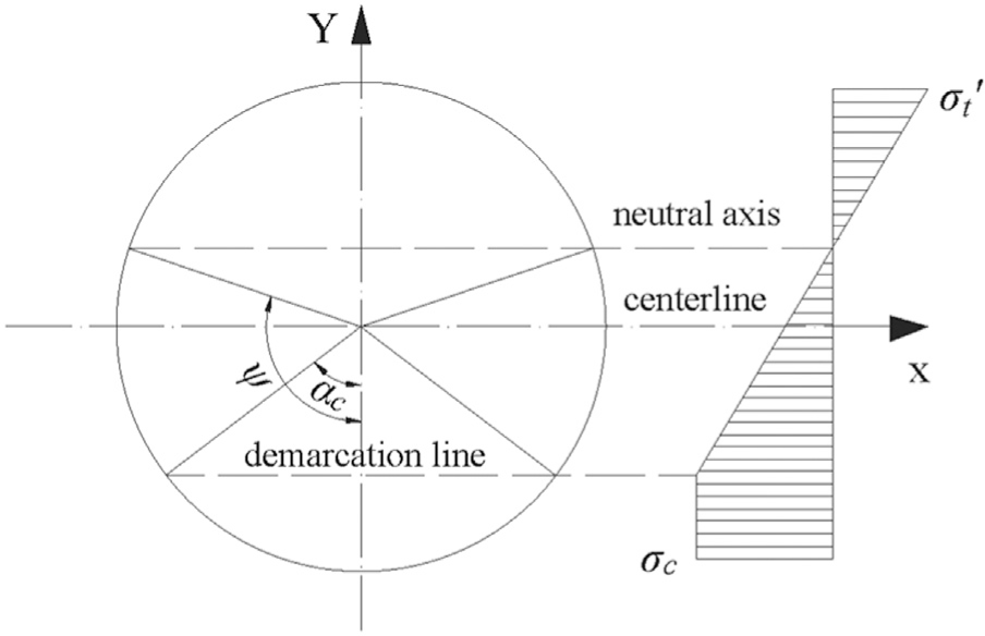
Stress distribution for Case 2.
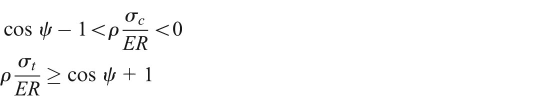
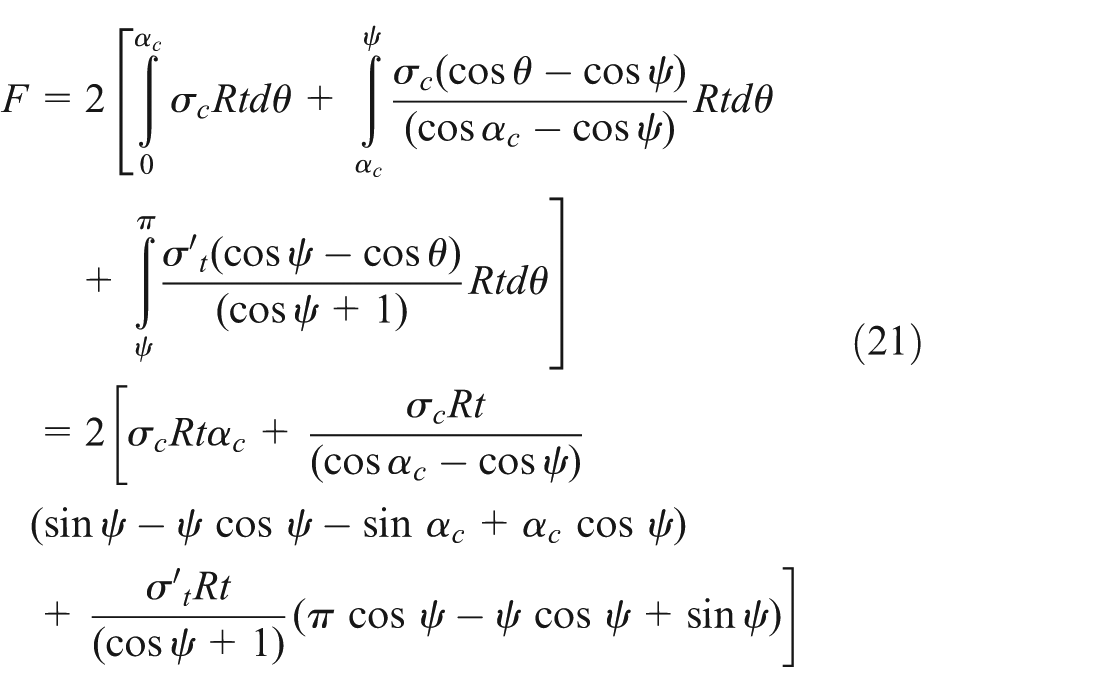
The axial force can be expressed as equation (21) for a pipe with the stress distribution as shown in Figure 9, in which
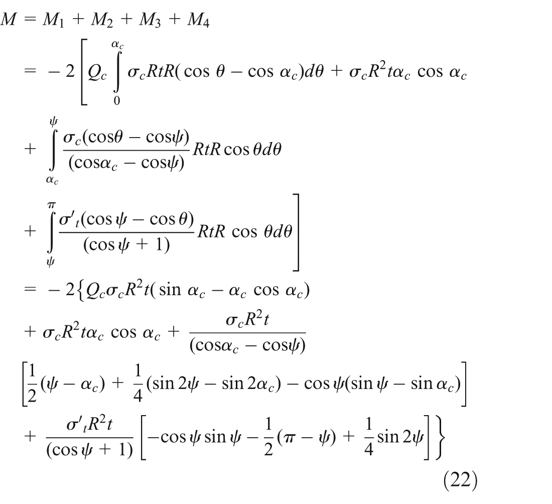
The influence of the ovalization of the compressive plastic region on the bending moment is determined from equation (12). For a given curvature radius
Case 3
This case represents only a portion of the tensile region reaching yield. Figure 10 shows the stress distribution of the pipe cross-section.
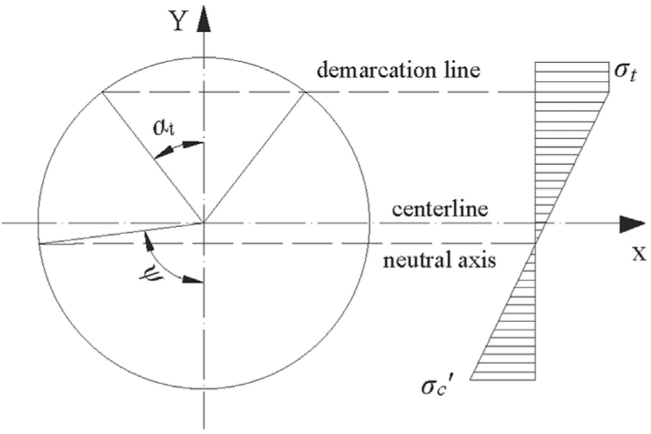
Stress distribution for Case 3.
The axial force for a pipe with the stress distribution shown in Figure 10 can be approximately expressed as equation (23), where the angle of
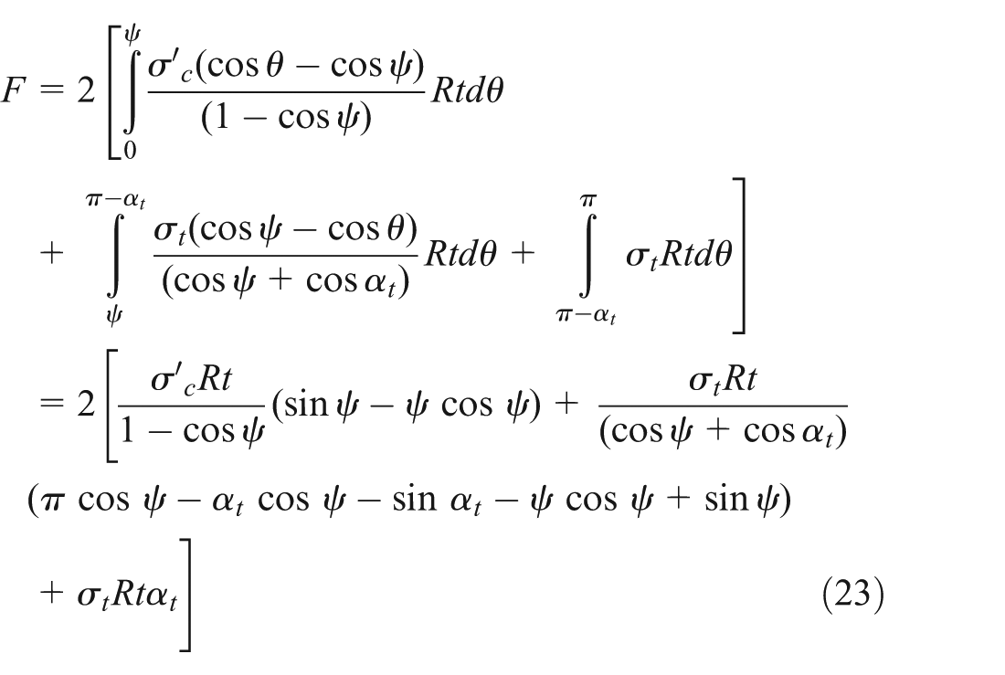
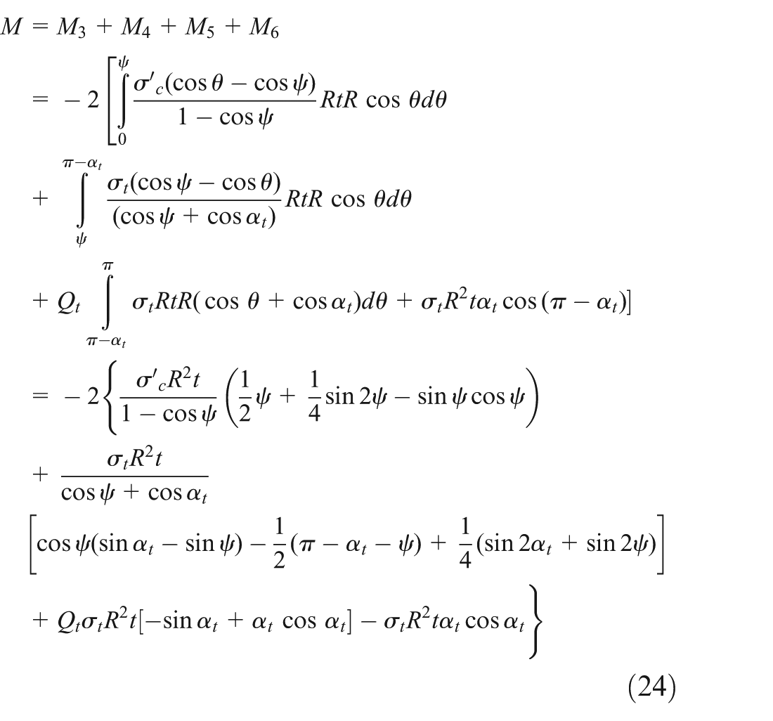
For the stress distribution shown in Figure 10, the influence of ovalization on the bending moment is determined from equation (12). For a given curvature radius
Case 4
Case 4 represents both portions of compressive and tensile regions reaching yield. Figure 11 shows the stress distribution of the pipe cross-section of Case 4.
Stress distributions for Case 4.
Similarly, the axial force can be expressed as equation (25) for a pipeline with a stress distribution as shown in Figure 11. The angle of the neutral axis
For the stress distribution displayed in Figure 11, the influence of ovalization on the bending moment is determined from equation (12). For a given curvature radius
The computational procedure
It is difficult to manually obtain the analytical solution from the above derived theoretical expressions. A program is developed using C++ language to determine the ultimate bending capacity, the relationship between the moment and curvature, and the parameters characterizing the deformation behavior of the pipe cross-section such as the location of the neutral axis, the compressed plastic region, and the tensioned plastic region.
At the initial stage of bending, a pipe has a lower bending moment and greater curvature radius
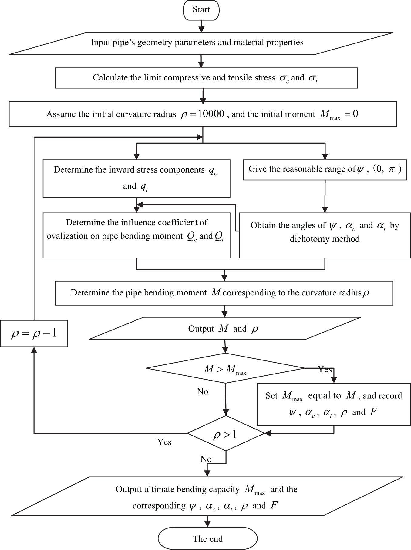
Flow chart of the computational procedure.
Verification
To obtain the bending moment of a pipe using the presented equations, the parameter
To verify the validity of the analytical solutions, the ultimate bending capacity and moment–curvature relationship of the steel pipes are investigated through the test and numerical methods below.
Test verification
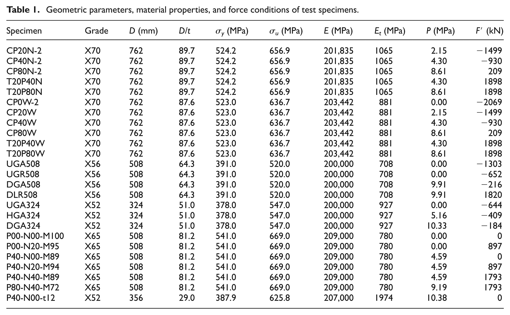
Experimental data from Dorey (2001), Mohareb (1995), Ozkan and Mohareb (2009), and Wang et al. (2014) are used to validate the analytical solutions proposed in this article. Table 1 lists the geometric parameters, material properties, and loading conditions of these tests, where
Geometric parameters, material properties, and force conditions of test specimens.
Comparison of pipe ultimate bending capacities
Table 2 compares the ultimate bending capacities of the test results and the analytical results proposed by Mohareb (2002, 2003) and this article, where the ratio represents the predicted result/test result.
Comparison of predicted ultimate bending capacity with test results (unit: kN m).
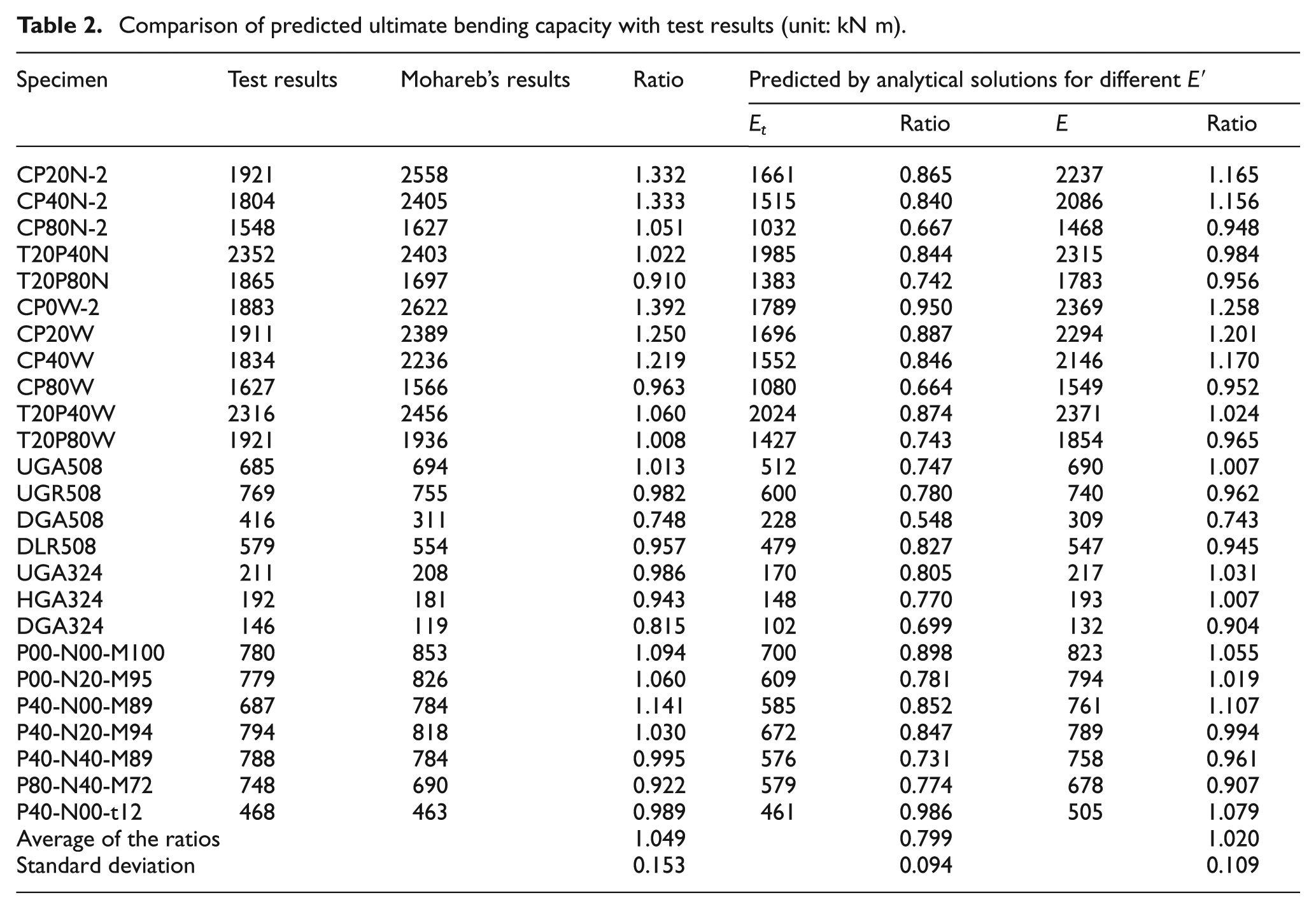
It can be seen from Table 2 that the average ratio of Mohareb’s results is 1.049, which is better than the lower (
The ratio of diameter to thickness is a significant factor for failure modes of steel pipelines subjected to combined loadings. Figure 13 shows the relationship between the diameter–thickness ratio and the ultimate bending capacity, where
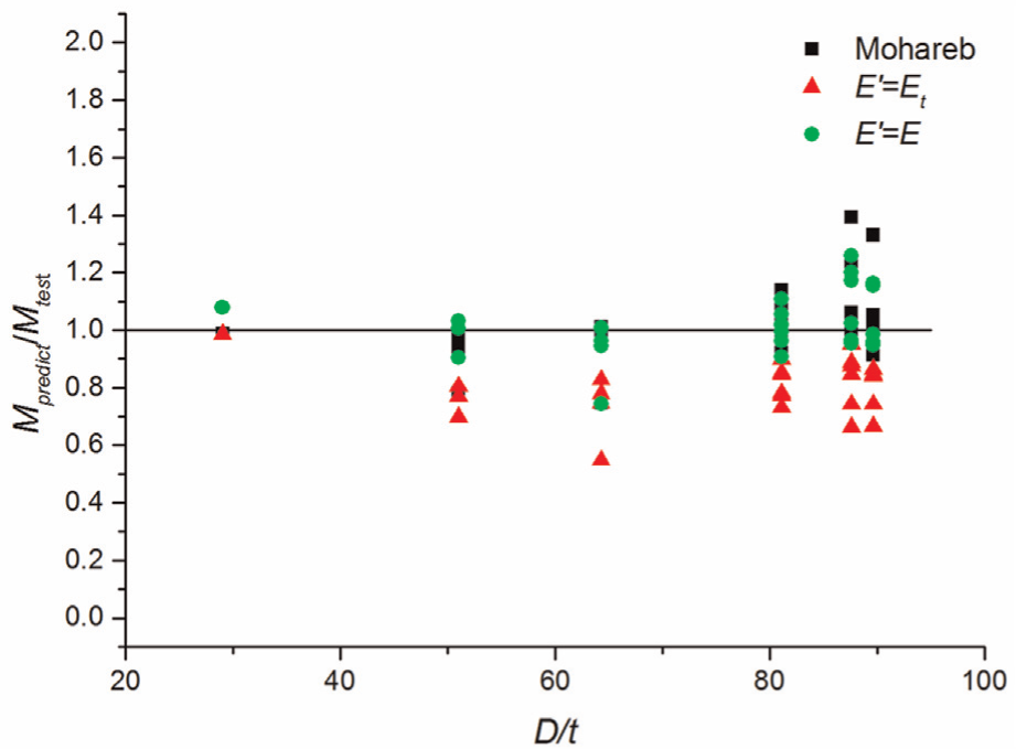
Relationship between diameter–thickness ratio and the ultimate bending capacity.
The influence of initial internal pressure on failure modes of steel pipelines subjected to bending moment is significant. Figure 14 displays the interaction between pipe bending capacities and initial loading conditions, where
Interaction between pipe ultimate capacities and loading conditions.
Moment–curvature relationship
Figure 15 shows the curves of global moment versus global curvature for four tests. The experimental curves are denoted by the solid black line; the red-dashed line represents the lower bound results with
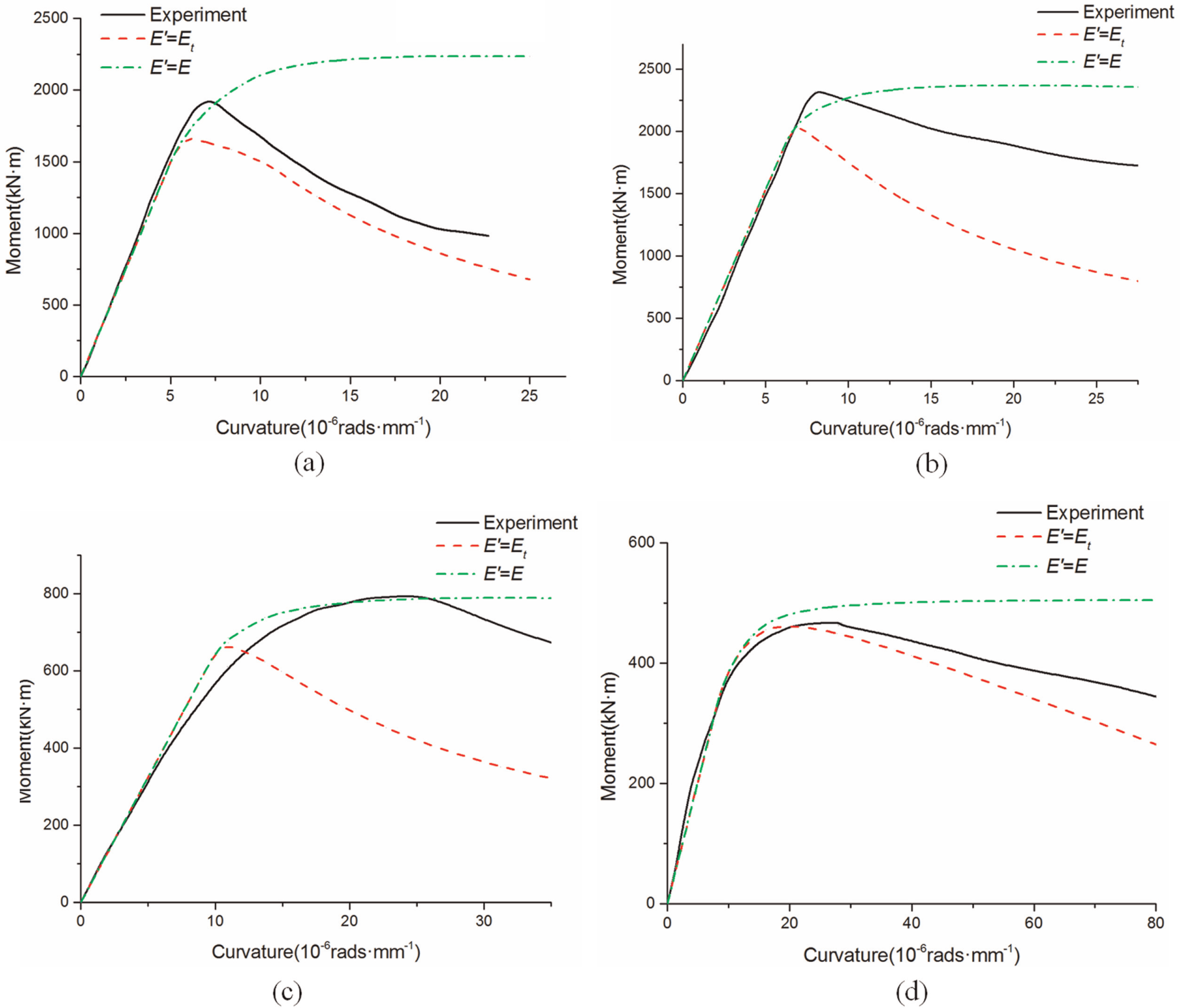
Global moment–curvature curves comparisons between theoretical derivation and tests: (a) CP20N-2, (b) T20P40W, (c) P40-N40-M94, and (d) P40-N00-t12.
As seen in Figure 15(a)–(d), both the moment–curvature curves of
Numerical verification
Based on the finite element method, numerical analysis of steel pipes is conducted to compare with the analytical solutions. The finite element analysis (FEA) simulator ABAQUS (ABAQUS, 2011) was selected to predict pipe behavior. Shell element S4R is adopted because it is efficient and reliable for large displacement, large rotation, and finite membrane strain shell analysis. A piecewise linear isotropic hardening stress–strain constitutive model, the von Mises yield criterion, and the associative flow rule were applied to describe the material behavior. The automatic Riks method is used to calculate the post-buckling of the steel pipe under monotonically increasing moment.
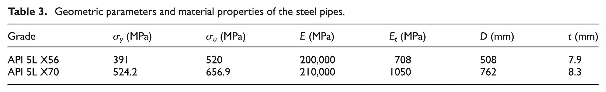
Two types of steel pipes are investigated through a numerical method and compared with the lower and upper bound solutions. Table 3 lists the geometric parameters and the material properties of the two types of steel pipes and the details of the true stress–strain curve are given in Dorey (2001) and Mohareb (1995). Determinations of the length of the pipes such as L/D = 2, 3.35, 5.31, 7.28, and 10 for X56, and L/D = 2.23, 3.54, 4.86, 7.22, and 10 for X70 are carried out. The results indicate that L = 2700 mm can ignore the boundary effects for both the two types of specimen. A mesh convergence study is also conducted for both the X56 and X70 specimens. The results of the study show that the 48 elements along the pipe circumference and 90 elements along the pipe axis for X56, and 60 by 90 elements for X70 can provide reliable bending capacities.
Geometric parameters and material properties of the steel pipes.
The finite element model should be validated first prior to studying the comparison of the numerical solutions with the analytical solutions. The test specimens UGA508 (Mohareb, 1995) and T20P80N (Dorey, 2001) are adopted to validate the finite element model. The finite element model of the specimen T20P80N is shown in Figure 16. The comparison of the global moment and curvature curve between the experimental and the FEA result is provided in Figure 17. From Figure 17, we can see that the finite element model can predict the ultimate capacity well, as well as the deformation behavior of pipeline. The errors of ultimate moment only −5.008% and 3.157%, respectively, where error = (FEA result − experiment result)/experiment result. Therefore, the finite element model can be used with confidence to validate the analytical solutions.
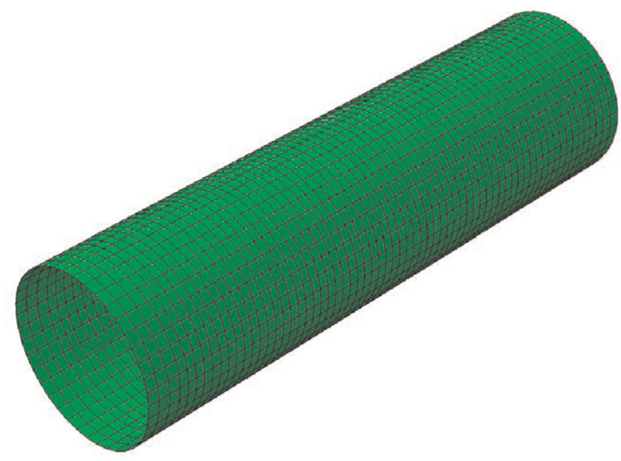
Finite element model of the pipe.
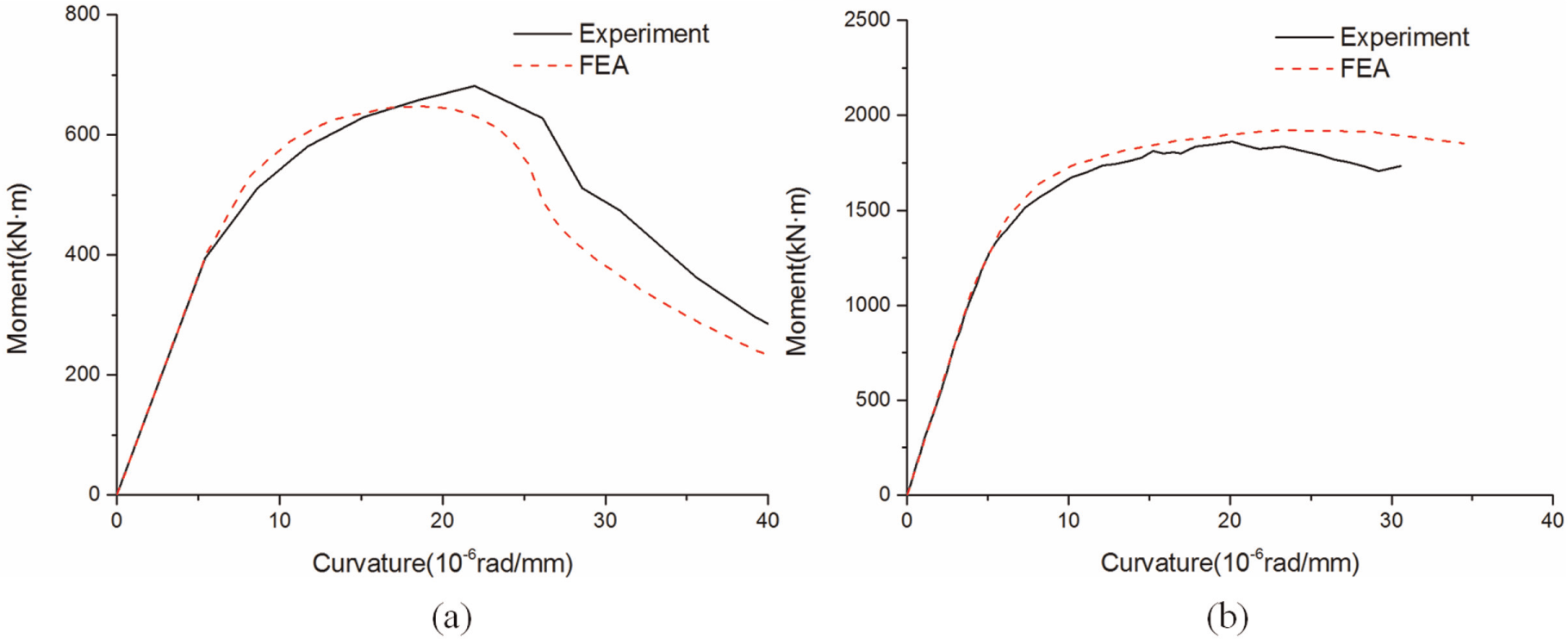
Comparison of global moment curvature curve: (a) UGA508 and (b) T20P80N.
Comparison of pipes ultimate bending capacities
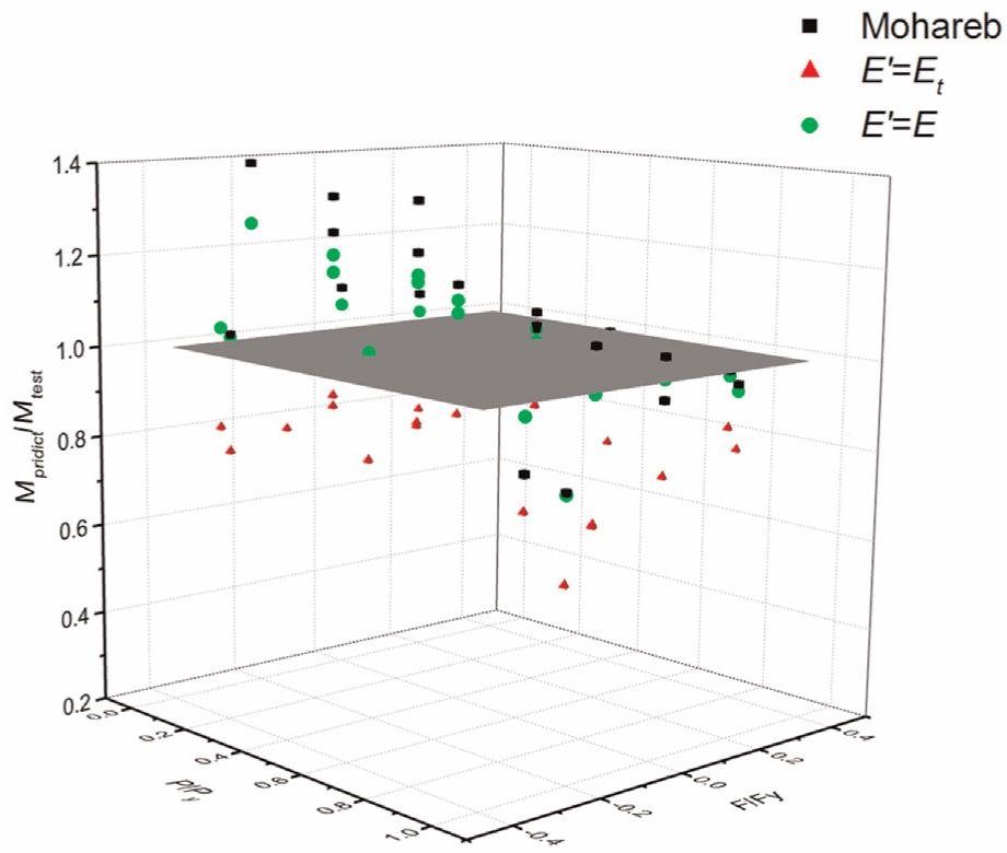
Figures 18 and 19 display the comparison of the ultimate bending capacities between the FEA, the analytical results proposed by Mohareb (2002, 2003), and the lower and upper bound solutions of this article under different internal pressures and axial forces, where

Comparison of the ultimate bending capacities for X56 pipes: (a) F/Fy = 0, (b) F/Fy = −0.2, (c) F/Fy = −0.4, and (d) F/Fy = −0.6.
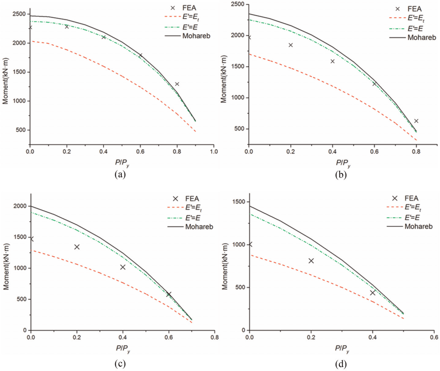
Comparison of the ultimate bending capacities for X70 pipes: (a) F/Fy = 0, (b) F/Fy = −0.2, (c) F/Fy = −0.4, and (d) F/Fy = −0.6.
From Figures 18 and 19, it can be seen that for the initial conditions with low axial force, the ultimate bending capacities from FEA are close to and lower than the upper and Mohareb’s solutions for most of X56 and X70 pipes. With the increase in axial force, the ultimate bending capacities predicted by FEA move away from the upper bound results and gradually closer to the lower bound results. The predicted results of the lower bound solutions are lower than the numerical results for any initial pressure and axial force. The FEA results lie between the lower and the upper bound solutions for most pipes, except for the X70 pipes with a high pressure. It is worth mentioning that axial forces are relatively low for most test specimens mentioned in section “Comparison of pipe ultimate bending capacities,” so the predicted bending capacities of the upper bound solutions agree quite well with test results.
Moment–curvature relationship
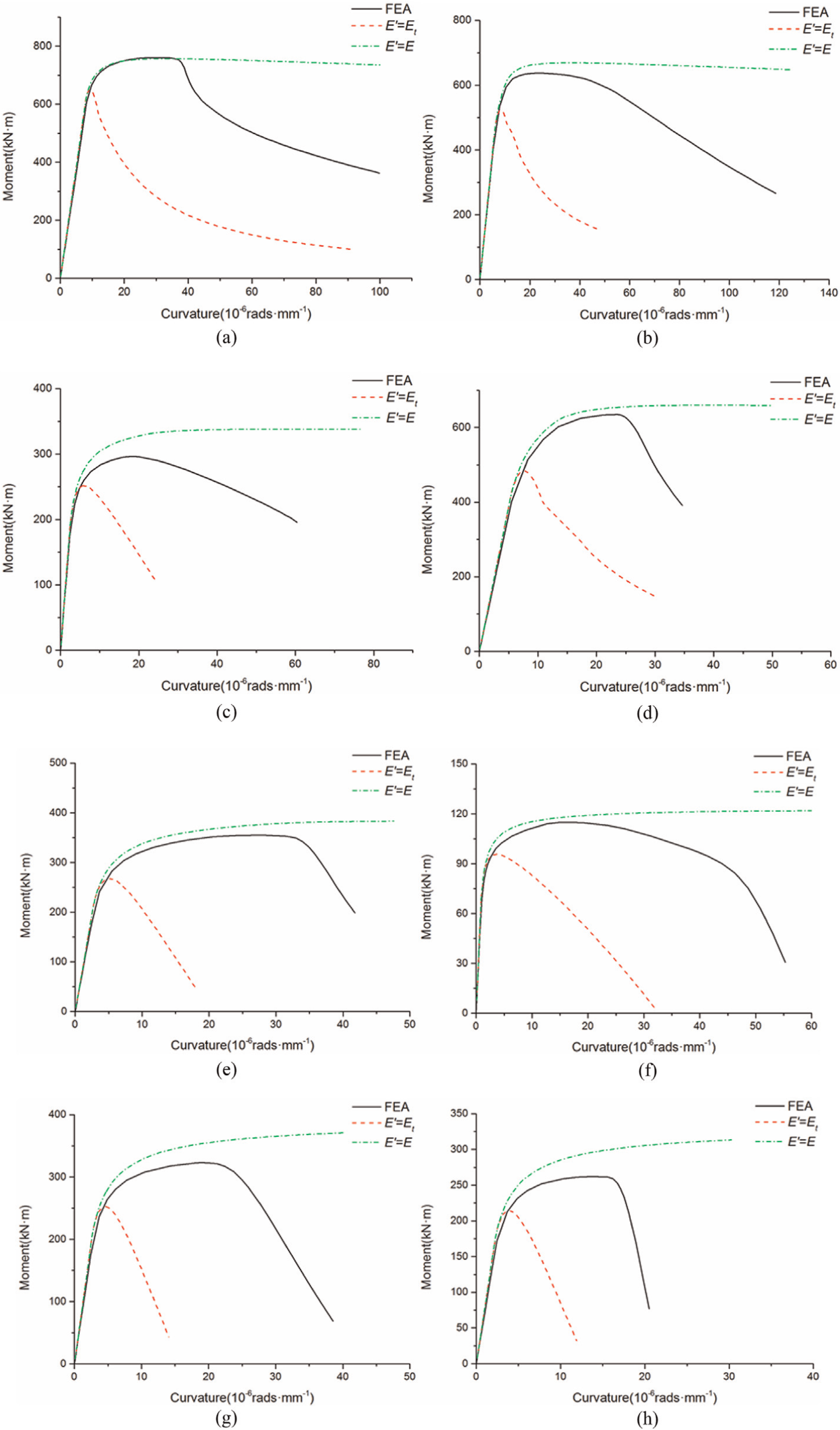
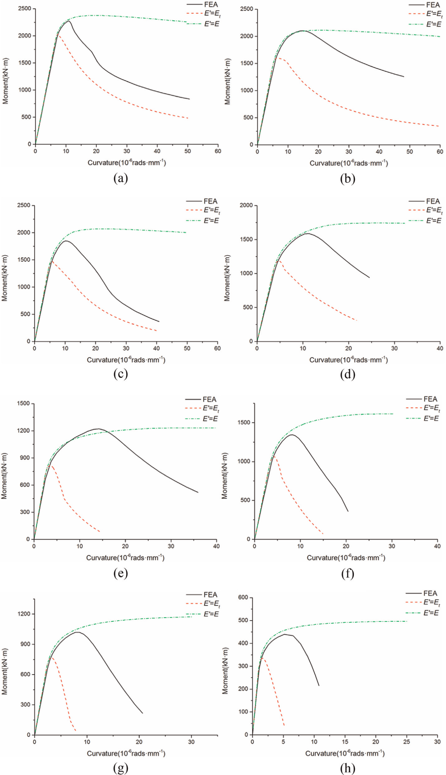
Figures 20 and 21 show the comparison of the moment–curvature curves between the numerical results and the upper and the lower bound solutions with different internal pressures and axial forces for X56 and X70 pipes. From these two figures, it can be seen that the moment–curvature curves for the FEA lie between the lower and upper bound curves for most of the pipes. During the elastic range, the curves of the FEA are completely consistent with those obtained from the lower and upper bound method. After entering the plastic range, the FEA moment–curvature curves depart from that predicted by the lower and upper bound curves as described in section “Moment–curvature relationship.” In the plastic range, the ultimate moment capacities of the lower bound solutions initially arose, followed by an apparent descending curve, and the longest yield plateau is observed for the upper bound solutions, with a slowly decreased curve.
Analytical and numerical moment–curvature curves for X56 pipes: (a) P/Py = 0, F/Fy = 0; (b) P/Py = 0.4, F/Fy = 0; (c) P/Py = 0.8, F/Fy = 0; (d) P/Py = 0.2, F/Fy = −0.2; (e) P/Py = 0.6, F/Fy = −0.2; (f) P/Py = 0, F/Fy = −0.4; (g) P/Py = 0.4, F/Fy = −0.4; and (h) P/Py = 0.2, F/Fy = −0.6.
Analytical and numerical moment–curvature curves for X70 pipes: (a) P/Py = 0, F/Fy = 0; (b) P/Py = 0.4, F/Fy = 0; (c) P/Py = 0.2, F/Fy = −0.2; (d) P/Py = 0.4, F/Fy = −0.2; (e) P/Py = 0.6, F/Fy = −0.2; (f) P/Py = 0.2, F/Fy = −0.4; (g) P/Py = 0.4, F/Fy = −0.4; and (h) P/Py = 0.4, F/Fy = −0.6.
Conclusion
Considering ovalization of the plastic region, the analytical solutions were derived for steel pipelines subjected to combined bending moments, axial forces, and internal pressure. The lower and the upper bound bending capacities were obtained, along with the relationship between the moment and curvature. In comparing the analytical results with the experimental and numerical results, the following conclusions can be drawn:
For the initial conditions with low axial forces, the predicted ultimate bending capacities of the upper bound solutions were close to and greater than the test and numerical results; with increased axial force, the upper bound results move away from the test and the numerical results. In general, the predicted ultimate bending capacities of the upper bound solutions agree quite well with experimental and numerical results; however, some of the cases are overestimated.
Under the initial conditions with low axial forces, there were some errors between the lower bound solutions and the results of experiments and FEA, and the errors decreased gradually with the increase in axial force. For the lower bound solutions, the bending capacities are underestimated for almost all of the test and numerical cases.
For the global moment versus global curvature curves of steel pipelines subjected to combined bending moments, axial forces, and internal pressure, both the lower and upper bound curves nearly matched those of the experimental and numerical results in the elastic range. As the curvatures increase, the moment–curvature curves predicted by the lower and upper bound solutions depart from the test and FEA results.
Footnotes
Declaration of conflicting interests
The author(s) declared no potential conflicts of interest with respect to the research, authorship, and/or publication of this article.
Funding
The author(s) disclosed receipt of the following financial support for the research, authorship, and/or publication of this article: This work was funded by the Chinese Ministry of Science and Technology (Grant No. 2011CB013702) and supported by the Program for New Century Excellent Talents in University (Grant No. NCET-11-0051).